A NASH BARGAINING SOLUTION TO MODELS OF TAX AND INVESTMENT
COMPETITION: TOLLS AND INVESTMENT IN SERIAL TRANSPORT CORRIDORS
Bruno De Borger, Wilfried PauwelsDocument de treball de l’IEB
2010/1
Documents de Treball de l’IEB 2010/1
A NASH BARGAINING SOLUTION TO MODELS OF TAX AND INVESTMENT COMPETITION: TOLLS AND INVESTMENT IN SERIAL TRANSPORT CORRIDORS
Bruno De Borger, Wilfried Pauwels
The IEB research program in Fiscal Federalism aims at promoting research in the public finance issues that arise in decentralized countries. Special emphasis is put on applied research and on work that tries to shed light on policy-design issues. Research that is particularly policy-relevant from a Spanish perspective is given special consideration. Disseminating research findings to a broader audience is also an aim of the program. The program enjoys the support from the IEB-Foundation and the IEB-UB Chair in Fiscal Federalism funded by Fundación ICO, Instituto de Estudios Fiscales and Institut d’Estudis Autonòmics.
The Barcelona Institute of Economics (IEB) is a research centre at the University of Barcelona which specializes in the field of applied economics. Through the IEB-Foundation, several private institutions (Caixa Catalunya, Abertis, La Caixa, Gas Natural and Applus) support several research programs.
Postal Address:
Institut d’Economia de Barcelona Facultat d’Economia i Empresa Universitat de Barcelona
C/ Tinent Coronel Valenzuela, 1-11 (08034) Barcelona, Spain
Tel.: + 34 93 403 46 46 Fax: + 34 93 403 98 32
http://www.ieb.ub.edu
The IEB working papers represent ongoing research that is circulated to encourage discussion and has not undergone a peer review process. Any opinions expressed here are those of the author(s) and not those of IEB.
Documents de Treball de l’IEB 2010/1
A NASH BARGAINING SOLUTION TO MODELS OF TAX AND INVESTMENT COMPETITION: TOLLS
AND INVESTMENT IN SERIAL TRANSPORT CORRIDORS * Bruno De Borger, Wilfried Pauwels
ABSTRACT: The purpose of this paper is to study toll and investment competition along a serial transport corridor competition allowing for partial cooperation between regional governments. Partial cooperation is modeled as a Nash bargaining problem with endogenous disagreement points. We show that the bargaining approach to partial cooperation implies lower tolls and higher quality and capacity investment than fully non-cooperative behavior. Moreover, under bargaining, strategic behavior at the investment stage induces regions to offer lower quality and invest less in capacity as compared to full cooperation. Finally, Nash bargaining partially resolves the problem of welfare losses due to toll and capacity competition pointed out in the recent literature.
JEL Codes: H71, H77, R48, R42
Keywords: Nash bargaining, tax competition, congestion pricing
Bruno De Borger Department of Economics University of Antwerp Prinsstraat 13 B-2000 Antwerp, Belgium Phone: + 32 3 2204161 Fax: + 32 3 2204799 E-mail: [email protected] Wilfried Pauwels Department of Economics University of Antwerp Prinsstraat 13 B-2000 Antwerp, Belgium Phone: + 32 3 2204185 Fax: + 32 3 2204799 E-mail: [email protected]
* The authors are in the Department of Economics, University of Antwerp. They are grateful to Peter Kort for
useful discussions, and to Marcel Weverbergh for executing the numerical example. The paper benefited from seminar presentations at the Universities of Barcelona (UB) and Lille. The University of Antwerp provided
Introduction
Tax competition between countries is a widely studied phenomenon in the public economics literature. Following up on the seminal paper by Mintz and Tulkens (1986), an extensive literature has been developed; important contributions include, among many others, Kanbur and Keen (1993), Wilson (1999), Janeba (2000), Zodrow (2003), Keen and Kotsogiannis (2003), Wilson and Wildasin (2004), and Borck and Pflüger (2006). The typical approach in these studies is to study the properties of the Nash equilibrium solution to the tax setting game, and to analyze the deviations from revenue or welfare maximizing behavior. This literature has convincingly shown that commodity or capital tax competition leads to inefficient tax setting behavior, and that the associated welfare losses may be large1.
Recently, tax and capacity competition has also been intensively studied in the transport economics literature. Simple parallel and serial transport networks have been considered in which different toll and capacity decisions for the different links of the network are made by different authorities (see, e.g., Levinson (2001), de Palma and Lindsey (2000), De Borger, Proost and Van Dender (2005), De Borger; Dunkerley and Proost (2007, 2008), and Ubbels and Verhoef (2008)). Several lessons can be drawn from this literature. First, toll competition between regions or countries implies that, independent of the network structure, tolls on through traffic will be inefficiently high. Second, competition between regions leads to too much capacity in parallel networks, whereas regions will substantially under-invest in serial transport corridors. In fact, if countries can toll through traffic, numerical analysis suggests that toll and capacity competition results in such a dramatic degree of tax exporting and underinvestment in capacity that it may be beneficial for a higher level government not to allow individual regions to toll at all (De Borger, Dunkerley and Proost (2007)). Third, tax exporting behavior holds both under a Nash and Stackelbergh approach to strategic interaction between regions (Ubbels and Verhoef (2008)).
1 However, given the large effects on tax rates typically found, some empirical studies have observed that
the welfare effects of tax competition are, at least under some sets of parameter values, surprisingly small (see, e.g., Sorensen (2000) or Parry (2003)).
With few exceptions, the above literature has studied tax competition assuming non-cooperative behavior between regions or countries2. This is somewhat surprising. It is well known that in the private sector firms have strong incentives to cooperate in at least some aspects of their decision-making3, and one expects these incentives to be at least as strong in the case of competition between regions or countries. After all, the inability to write legal and binding contracts – one of the main reasons for the type of Nash competition typically assumed – is probably less pronounced in the case of national or regional governments than it is for private firms. Hence, the prisoner’s dilemma is much less likely to prevent cooperation than in the private sector.
The purpose of this paper is, therefore, to study competition between regions in a framework that allows for partial or full cooperation between regional governments. For purposes of concreteness, the model is framed in a setting of toll and investment competition between regions along a serial transport corridor. This focus on the transport sector is no coincidence. First, the fact that transport decisions involve both long-run (e.g., capacity) and short-run (e.g., prices, tolls) decisions implies substantial potential for partial cooperation. Second, in practice, cooperation and bargaining are observed to be important characteristics of national or regional decision-making in pricing and investment4. The importance of pure transit traffic and the high congestion levels observed in many European countries not only implies that any country’s decision on tolls or capacities has international implications, but it also placed congestion problems high on the political agenda. Frequent international contacts between top politicians then make negotiated outcomes quite realistic.The same holds at the local, urban level. Many large urban areas throughout Europe have massive commuting by non-urban residents towards the city center. City and regional governments make decisions on investment and
2 One recent exception is Han and Leach (2008). In their model, competing governments bargain with
individual firms over financial incentives to attract them to their jurisdiction. They show that this individual bargaining framework yields results that differ substantially from the standard tax competition model. Under some specifications of the model tax competition does not imply capital misallocation. The Han-Leach paper is totally unrelated to the bargaining model of the current paper.
3 See, for example, d’Aspremont and Jacquemin (1988), Fershtman and Muller (1986), Brod and
Shivakumar (1999), and Savanes, Steen and Sorgard (2003).
4 Of course, the nature of cooperation depends on the type of problem and may cover a wide range of
policies. For example, financing concerns and relative benefits often drive negotiations over cross-border infrastructure projects (e.g., the discussion about deepening of the river Scheldt between Belgium and the
potential tolling of city access. Negotiating about the distribution of potential future toll revenues is often an important ingredient of the political discussion between cities and regional or national authorities.
We study a two-stage model of toll and investment decisions by regions along a serial network, as in De Borger, Dunkerley and Proost (2007) and Ubbels and Verhoef (2008). Both investment in ‘quality’ (e.g., maintenance) and capacity (e.g., extra lanes) are considered. Unlike previous papers, we allow for partial cooperation between regions. Following Pauwels and Kort (2008), partial cooperation is modeled as a Nash bargaining problem with endogenous disagreement points. This setup assumes that regions can strategically use quality or capacity investments to strengthen their bargaining position prior to negotiating over toll levels and the distribution of the total payoff5. The model assumes that countries cooperate at the tolling stage and negotiate over the distribution of the payoff knowing that, if no bargaining agreement is reached, they fall back at the Nash equilibrium of the non-cooperative tolling game. At the capacity stage of the game, countries compete in order to ensure a better bargaining position and to get a larger share of the net payoff.
Findings of this paper include the following. First, in a model of toll and quality choices, we show that regions’ relative bargaining positions are independent of congestion; they positively depend on the cost of quality. In other words, the region where the cost of quality is higher has the strongest position. Second, considering a model of toll and capacity decisions we find that a region’s pre-bargaining position negatively depends on both the intensity of congestion (more specifically, on the slope of the congestion function) and on the cost of capacity. Third, partial cooperation implies lower tolls and higher quality and capacity investment than under the full Nash equilibrium in both tolling and investment. Finally, Nash bargaining yields higher
5 In a recent extension of models of semi-collusion in industrial organization (see, e.g., Brod and
Shivakumar (1999)), Pauwels and Kort (2008) consider a model where in the first stage firms spend on R&D in a Nash competitive setting while, at the second stage, they bargain over the distribution of joint profits. The outcome of the Nash bargaining game in outputs is considered as the threat point. They show that investment in the first stage is motivated by: (i) raising joint profits at the second stage; (ii) strengthening the bargaining position. They consider semi-collusion, full cooperation at both stages, full competition (i.e., a Nash game is played at both stages), and they provide some introductory comparative analysis.
welfare than full Nash competition. Partial cooperation therefore partially resolves the problem of welfare losses associated with fierce toll and capacity competition pointed out in the recent literature (see, e.g., De Borger et al. (2007)).
The remainder of this paper is organized as follows. In Section 1 we present an intuitive introduction to the Nash bargaining approach used in this paper. Section 2 studies two models of road transport investment (‘quality’ and ‘capacity’, to be defined more precisely below), assuming the objective of regions is to maximize toll revenues. We compare the results of partial cooperation with those obtained in the Nash equilibrium in both tolls and qualities or capacities. In Section 3, we extend the model to a setting in which regions are not only interested in net toll revenues but also care about the welfare of road users. Section 4 provides a simple numerical example. Finally, Section 5 concludes.
1. Cooperation and Nash bargaining in toll-capacity games: some preliminaries
Nash (1950) suggested an axiomatic approach to cooperative games in which parties cooperate in maximizing the total joint payoff, but where bargaining takes place over the distribution of this payoff. The Nash bargaining solution implies that parties receive a share of the total payoff that is determined by their relative ‘disagreement’ levels, defined as the payoffs they receive if cooperation fails.
In general, a Nash bargaining problem is defined by a pair ( , (F dA,dB)), where F is the set of feasible payoffs of the two players, and (dA,dB) is the disagreement point. Let the set F of feasible combinations be defined by
{
2}
( A, B) A B
F ϕ ϕ ∈R ϕ +ϕ ≤ϕ
where ϕ ϕA, B are the payoffs for region A and B, respectively, and ϕ is the maximal value of the total payoff that can be achieved by cooperation. Note that the feasible set describes all possible combinations of dividing ϕ between the two players. Nash shows that the solution to the bargaining problem yields the following payoffs for players A and
{
}
{
}
0.5 0.5 A B B A d d d d ϕ ϕ + − + −Intuitively, the bargaining solution implies that each player receives half of the joint total payoff if their fallback positions are the same; if this is not the case, the player with the more favorable bargaining position gets more than half.
In this paper, we study partial cooperation as a Nash bargaining problem in the following concrete setting. Assume there are two regions, A and B, located along a serial transport corridor. Assume for simplicity that all traffic passes through the two regions and that there is no traffic just traveling in one of the regions6. Moreover, we consider a single direction. Figure 1 illustrates the situation. Total demand is denoted by X. The regions have each two policy instruments and face a two stage decision process: they have to decide on a short-run variable (t ii =A B, )(e.g., tolls) and a long-run variable
( , )
i
q i=A B (e.g., road capacity). Note that the description illustrated by Figure 1, although very simple, does capture the basics of a number of realistic problems. For example, it describes toll and capacity competition between countries that suffer to a large extent from through traffic (see De Borger, Dunkerley and Proost (2007)). Alternatively, it provides a simplified description of a city and a surrounding region; commuters travel from the region into the city every morning. The city and the regional government have to make decisions on road investment and on toll access charges into the city center (Ubbels and Verhoef (2008)).
Traffic Flow X
Region A Region B
Figure 1: A simple serial transport corridor
6 Introducing local transport in both regions, which is obviously more realistic, complicates the model
Within this setting, an intuitive description of the approach taken in this paper is as follows. Let the objective functions (this can be toll revenue, welfare, etc.) in regions A and B be written in general as functions of tolls and investment levels in both regions, respectively:
( , , , ), ( , , , )
A t t q qA B A B B t t q qA B A B
ϕ ϕ .
Although other configurations could be conceived7, we assume in this paper that regions cooperate at the tolling stage and negotiate over the distribution of payoffs. However, following Pauwels and Kort (2008) -- and unlike the original bargaining problem -- it is assumed that the disagreement levels of the bargaining problem are not exogenous, but are endogenously determined by regions’ strategic investment behavior. Specifically, regions know that, if no bargaining agreement is reached, they fall back at the Nash equilibrium of the non-cooperative tolling game. This disagreement point, however, can be manipulated by regions’ investment decisions. At the investment stage of the game, countries therefore compete in order to ensure a better bargaining position and to get a larger share of the net payoffs of the policy. The Nash bargaining model considered here then implies that, on the one hand, regions have an incentive to determine investment to maximize their joint total payoff but, on the other hand, by threatening to play non-cooperatively, they also use investment decisions to secure a better bargaining position when negotiating about the distribution of the joint payoff between regions.
To model the process just described, at the tolling stage, regions maximize the joint total payoff, for given investment levels in the two regions:
, ( , , , ) ( , , , )
A B
A A B A B B A B A B t t
Max ϕ t t q q +ϕ t t q q
If negotiations fail, regions fall back at the disagreement point. This is the non-cooperative Nash equilibrium in tolls, yielding payoffs of ϕANE(q qA, B),ϕBNE(q qA, B), respectively. This Nash equilibrium is obtained by assuming each region maximizes its
7 Indeed, partial cooperation could also take the form of cooperation at the investment stage and
competition at the tolling stage, the opposite of what we assume here. The former could make a lot of sense in the case of cross-border infrastructure projects, where different countries cooperate on investment decisions but have non-cooperative tolling strategies. The case analyzed in this paper, viz. cooperation at the tolling stage and investment competition may be more plausible for the interaction between a city and regional government that cooperate when tolling city access, but have individual investment strategies. For a private sector application of a model of partial cooperation where cooperation is at the R&D stage and
own payoff with respect to the toll it controls, treating investment levels and the toll level in the other region as exogenously given. The disagreement payoffs determine the strength of the bargaining positions in the investment game. In the second stage, capacities are determined non-cooperatively. Given Nash’s solution (1950) to the toll bargaining game, regions A and B can be assumed to determine investment so as to solve, respectively:
{
}
{
}
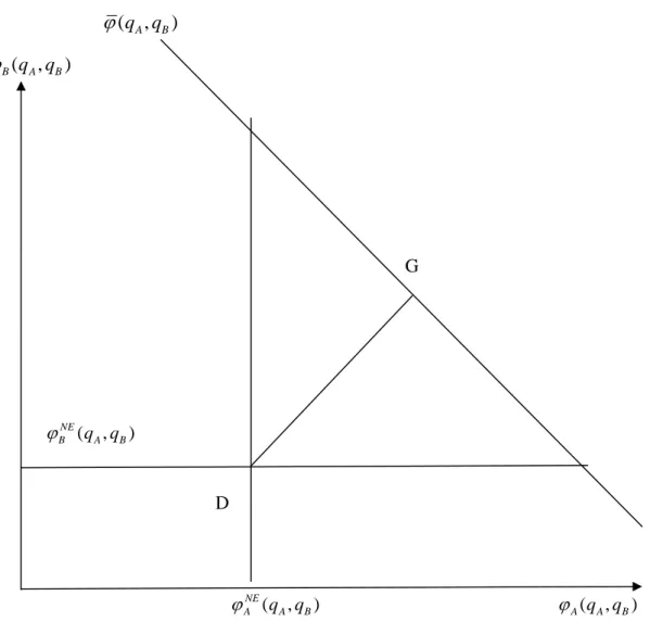
* * ( , ) 0.5 ( , ) ( , ) ( , ) ( , ) 0.5 ( , ) ( , ) ( , ) A B NE NE A A B A B A A B B A B q NE NE B A B A B B A B A A B q Max q q q q q q q q Max q q q q q q q q ϕ ϕ ϕ ϕ ϕ ϕ ϕ ϕ = + − = + −The Nash bargaining concept used in this paper is illustrated on Figure 2. On the axes, we have the values of the payoff functions of the two regions. The set of all possible divisions of the maximal joint payoff (ϕ q qA, B) is depicted by the linear relation with slope minus one. The disagreement point D is also indicated; the vertical and horizontal lines denote ϕANE(q qA, B)and ϕBNE(q qA, B), respectively. Finally, the Nash bargaining solution is given by the point G. The intuition of the model is clear. On the one hand, regions have an incentive, by appropriate investment, to raise the maximal joint payoff ϕ(qA,qB). This shifts the linear relation with slope minus one to the right. On the other hand, investment decisions affect the disagreement point, so regions use investment to ensure a better bargaining position and to get a larger share of the joint payoff. For example, if region A succeeds in shiftingϕANE(qA,qB)to the right, point G moves to the right, reflecting a better outcome for A.
(q qA, B)
ϕ
( , ) B q qA B ϕ G ( , ) NE B q qA B ϕ D ( , ) NE A q qA B ϕ ϕA(q qA, B)Figure 2. The Nash bargaining solution.
2. Nash bargaining with revenue maximizing governments
In this section, we study Nash bargaining as partial cooperation in the two-stage toll-investment model described in Section 1, assuming that the regions’ payoffs are total (net of investment cost) toll revenues. We derive information on investment and toll
levels, and compare with the outcomes under full cooperation and fully non-cooperative behavior (i.e., Nash competition at both decision stages).
We analyze the model for two different and highly stylized types of investment in transport infrastructure. One type of investment reduces the average cost of making a trip, independent of the traffic flow. Think of road pavement quality choice, road maintenance, highways lights, and traffic light coordination as stylistic examples. Better pavement quality reduces travel cost, independent of the traffic flow; the same holds for better maintained roads. We refer to this first type of investment as ‘quality’. The second type of investment is a ‘capacity’ expansion; the degree to which this reduces the cost of making a trip varies with the traffic flow using the road: the user cost reduction only materializes when there is more traffic. The cost at free flowing traffic levels is not affected.
2.1. Maximizing toll revenues: toll and road quality choice under Nash bargaining
Regions make decisions on ‘quality’ (broadly defined, see above, but excluding pure capacity increases) and toll levels. They only care about toll revenues, net of investment expenses. We use simple demand and cost specifications throughout. Demand is linear and given by
( )
X
p X = −a bX (1)
Generalized cost functions are also assumed to be linear. To keep the analysis as tractable as possible, we specify the (net of toll) cost of making a trip of given distance in regions A and B as, respectively:
( , ) ( ) ( , ) ( ) A A A A A B B B B B C X m m X C X m m X α β α β = − + = − + (2)
The average money plus time cost of making a trip is a linear function of the traffic flow X; the slopes of the cost functions β βA, B reflect the severity of extra traffic for congestion. Investment in road quality (m m ) is assumed to reduce the cost of making A, B
a trip independent of the traffic volume. It reduces the cost of free flowing traffic. We impose mi<αi (i=A B, ).
( ) (.) (.)
X
A A B B
p X =C + +t C + t (3) This leads to the ‘reduced-form’ demand function for traffic as a function of tolls and qualities in both regions. We find:
( ) ( ) ( , , , ) A B A A B B , A B A B A B a t m t m X t t m m N b N α α β β − − − − − − = = + + (4) A. Nash bargaining
As argued above, regions cooperate at the tolling stage and bargain over the distribution of total net revenues realizing that, when no agreement is reached, they fall back at the non-cooperative Nash equilibrium. Prior to bargaining they use quality investments strategically as a way to secure a more powerful negotiating position.
Nash bargaining: the tolling stage
Regions maximize joint (net of maintenance expenditures) toll revenues:
[
]
2 2 , ( ) ( , , , ) 0.5 ( ) 0.5 ( ) A B A B A B A B A A B B t t Max t +t X t t m m − γ m − γ mwhere X(.) is reduced-form demand as given above. It is assumed that quality investment costs are quadratic in quality levels.
Not surprisingly, given the structure of the problem the optimal tax rates are not separately identified. What matters for overall demand is just the total toll level for the whole trip. Using the reduced-form demand function the first-order condition immediately implies:
( )
A B A B
t + = +t b β +β X (5) This immediately implies that the overall toll level exceeds the global marginal external congestion costs; the latter is easily seen to equal (βA+βB)X. Substituting demand (4) into (5) and working out, the total tax to pass through the two regions is given by:
2
NB NB A B A B A B
a m m
Joint toll levels are rising in road quality levels, but independent of congestion functions’ slope parameters. Combining (5) and (6), we see that optimal demand is rising in road quality but declining in congestion severity, as captured by the slope parameters:
2 2( ) A B A B A B A B A B a m m a m m X N b α α α α β β − − + + − − + + = = + + (7)
Total toll revenues net of capacity costs equal, after substituting in the objective function: 2 2 2 1 ( , ) 0.5 ( ) 0.5 ( ) 2 A B A B A B A A B B A B a m m m m m m b α α ϕ γ γ β β ⎛ ⎞⎡ − − + + ⎤ =⎜ ⎟ ⎢ ⎥ − − + + ⎣ ⎦ ⎝ ⎠ (8)
This is the overall optimal toll revenue minus investment costs in both regions; it obviously depends on investments in both regions.
Nash bargaining: the disagreement point
If regions do not succeed in attaining a bargained outcome which is acceptable to both parties, the outcome of the process is the region’s fallback position. This fallback or disagreement point is assumed to be the non-cooperative Nash equilibrium in tolls. To analyze this disagreement level, note that country A solves:
[
]
2 ( , , , ) 0.5 ( ) A A A B A B A A t Max t X t t m m − γ mholding quality levels and toll levels in B constant. Country B behaves in a similar fashion. The reaction functions are:
2 2 A B A B B A A B A B A B a m m t t a m m t t α α α α − − + + − = − − + + − =
Tolls in a region are declining in the toll level in the other region. Solving the set of reaction functions yields the unique (and stable: slopes equal -0.5) Nash equilibrium toll solution: 3 NE NE A B A B A B a m m t =t = −α −α + + (9)
The joint toll payment to travel through both regions exceeds the cooperative toll level, conditional on quality (compare (9) with (6)). The net revenue levels at the Nash disagreement points are, for regions A and B, respectively:
2 2 2 2 1 ( , ) 0.5 ( ) 3 1 ( , ) 0.5 ( ) 3 NE A B A B A A B A A A B NE A B A B B A B B B A B a m m m m m b a m m m m m b α α ϕ γ β β α α ϕ γ β β ⎛ ⎞⎡ − − + + ⎤ =⎜ ⎟ ⎢ ⎥ − + + ⎣ ⎦ ⎝ ⎠ ⎛ ⎞⎡ − − + + ⎤ =⎜ ⎟ ⎢ ⎥ − + + ⎣ ⎦ ⎝ ⎠ (10)
The pre-bargaining quality investment game
Nash bargaining implies that region A, at the pre-bargaining stage, chooses its quality level so as to:
{
}
* 1 ( , ) ( , ) ( , ) ( , ) 2 A NE NE A A B A B A A B B A B m Max ϕ m m = ϕ m m +ϕ m m −ϕ m m (11) The implicit assumption is that country A will get half of the total maximum jointrevenues if both regions have equal bargaining strength. The strength of the bargaining position is captured by the relative revenues for the two regions at their respective Nash equilibrium disagreement points.
Observe that region A can strategically use optimal quality investment at the pre-bargaining stage to raise its pre-bargaining position. Indeed, (10) implies:
NE NE A B A A A A m m m ϕ ϕ γ ∂ −∂ = − ∂ ∂
Interestingly, this means that region A strengthens its bargaining position by offering less road quality. Doing so has two effects: it reduces costs, raising region A’s net revenues at the fallback position; it also reduces demand for transport, but this affects the Nash equilibrium fallback position for A and B in an identical manner and, hence, does not affect relative bargaining strength. Conditional on a given quality, regions A’s bargaining power is also reduced when its quality cost increases.
Using the specification of the various functions derived above (see (8) and (10)), the first order condition for A’s optimal quality choice problem (11) at the pre-bargaining stage implies the following reaction function, derived after simple algebra:
1 4 1 4 1 A B A B A A a m m N N α α γ γ − − = + − −
Reaction functions are upward sloping by the second-order conditions. If one country raises quality investment it pays for the other to do so as well in order to generate extra traffic and toll revenues. A similar problem is solved by B. Solving for the Nash equilibrium qualities yields:
( ) 4 ( ) ( ) 4 ( ) NB B A B A A B A B NB A A B B A B A B a m N a m N γ α α γ γ γ γ γ α α γ γ γ γ − − = − + − − = − + (12)
The joint toll level at the Nash bargaining solution is easily calculated, using (12) in expression (6). We obtain: 2 ( ) 4 ( ) NB NB A B A B A B A B A B N a t t N γ γ α α γ γ γ γ − − + = − + (13)
Demand is given by, using (5) and (12):
2 ( ) 4 ( ) NB A B A B A B A B a X N γ γ α α γ γ γ γ − − = − +
Note that demand both directly determines congestion and overall consumer surplus for the users8. Finally, total joint revenues are:
[
]
[
]
2 2 ( ) 1 8 ( ) 2 4 ( ) NB A B A B A B A B A B A B a N N γ γ α α ϕ γ γ γ γ γ γ γ γ ⎧ − − ⎫ ⎪ ⎪ = ⎨ ⎬ − + − + ⎪ ⎪ ⎩ ⎭ (14)We are now in a position to study in more detail the determinants of the pre-bargaining position for region A. To do so, let us substitute the optimal quality levels (12) into NE NE
A B
ϕ −ϕ , using (10). Working out, straightforward algebra shows that A’s position is stronger than B’s if and only if γA >γB. This has two implications. First, surprisingly, the region with the highest cost parameter has the strongest position. The intuition is as follows. Expression (10) shows that quality choices do not matter for revenues (the first
8 Indeed, it is easily shown that the surplus of users, i.e.,
(
)
0 ( ) (.) X X X p z dz− g X
∫
is directly proportional to demand squared.term on the right hand sides of (10) are identical for both regions) in this model, and the higher quality cost in region A induces it to offer a lower quality than B. This yields lower quality costs for region A, raising its net revenues and, hence, raising its bargaining power. The trade off for a region is this: if it invests more in quality, it raises total demand and joint toll revenues, but it also reduces its bargaining position, hence it gets less of a larger amount. Second, note that relative congestion parameters do not matter at all for bargaining positions.
B. Full cooperation at both capacity and tolling stages
It will be instructive to compare the Nash bargaining solution with the fully cooperative outcome. Suppose regions cooperate at both the tolling and quality stages. If the two countries cooperate at both stages, they maximize joint net toll revenues (8) with respect to both investment levels. Solving yields the optimal fully cooperative investment levels: ( ) 2 ( ) ( ) 2 ( ) FC B A B A A B A B FC A A B B A B A B a m N a m N γ α α γ γ γ γ γ α α γ γ γ γ − − = − − − − = − − (15)
Tolls at the full cooperative equilibrium are:
[
( ) (]
) 2 A B A B FC FC A B A B A B N a t t N γ γ α α γ γ γ γ − − + = − − (16) Demand is:[
]
( ) 2 A B A B FC A B A B a X N γ γ α α γ γ γ γ − − = − − (17)Total net toll revenues are:
(
)
2 ( ) 1 2 2 FC A B A B A B A B a N γ γ α α ϕ γ γ γ γ ⎡ − − ⎤ = ⎢ − − ⎥ ⎣ ⎦ (18)C. Nash equilibrium in both tolls and quality: full competition
Finally, let us compare with full non-cooperative behavior at both stages. If countries compete in both tolls and investment, then each region maximizes its Nash
equilibrium profit, obtained for the Nash equilibrium tolls, conditional on quality investment levels. These were given by (10). Solving for the Nash equilibrium, we find the following capacities:
2 ( ) 9 ( ) 2 2 2 ( ) 9 ( ) 2 2 NE B A B A A B A B NE A A B B A B A B a m N a m N γ α α γ γ γ γ γ α α γ γ γ γ − − = − − − − = − − (19)
Tolls at the Nash equilibrium are easily derived as:
[
3]
( ) 9 ( ) 2 2 A B A B NE NE A B A B A B N a t t N γ γ α α γ γ γ γ − − = = − − (20)Moreover, demand is found to be:
[
3]
( ) 9 ( ) 2 2 A B A B NE A B A B a X N γ γ α α γ γ γ γ − − = − − (21)Finally, total net toll revenues are calculated to be:
[
]
[
]
2 ( ) 9 ( ) 2 2 A B A B NE A B A B a N γ γ α α ϕ γ γ γ γ − − = − − (22) D. Comparison of regimesThe various expressions for tolls, quality and demand are summarized in Table 1 for the different regimes. Simple algebra then shows that the relations given in Table 2 hold.
Interpretation is straightforward. First, quality investment is highest under full cooperation, and it is higher under Nash Bargaining than under full competition. The reason that it is lower under bargaining than under full cooperation is that regions strategically provide lower quality to strengthen pre-their bargaining position when negotiating over net toll revenues. Second, the total toll to travel through regions A and B is highest under full competition. Interestingly, the total toll is lowest under Nash bargaining. Although full cooperation and bargaining imply the same toll rules, conditional on quality, investment in quality is higher under full cooperation. Higher quality implies higher overall tolls, see before. Demand (and hence congestion and consumer surplus) is highest under full cooperation, despite the fact that regions
maximize net revenues. It is lowest under full competition. Finally, total net revenues under bargaining are higher than under full competition.
This leads to three clear conclusions. First, bargaining leads to more favorable outcomes than non-cooperative behavior: it yields lower tolls, higher quality, higher net consumer surplus and higher overall welfare9. Second, strategic use of quality investment does under bargaining imply that bargaining performs less favorable that full cooperation. Third, despite the fact that regions maximize net toll revenues, both partial and full cooperation are better for road users than non-cooperative behavior.
9 The nature of the model, involving bargaining and congestion externalities, implies that the results are
more clear cut than in models of semi-collusion considered in the industrial organization literature. There it is often found that whether an output cartel (partial cooperation on the output market) is good for consumers and/or producers depends on the size of spillover effects of investment. See, e.g., Feshtman and
Table 1: summary of findings
Nash Bargaining (NB) Full cooperation (FC) Full Nash competition (N Quality ( ) 4 ( ) ( ) 4 ( ) NB B A A B A B NB A B A B A B J m N J m N γ γ γ γ γ γ γ γ γ γ = − + = − + ( ) 2 ( ) ( ) 2 ( ) FC B A A B A B FC A B A B A B J m N J m N γ γ γ γ γ γ γ γ γ γ = − − = − − 2 ( ) 9 ( ) 2 2 2 ( ) 9 ( ) 2 2 NE B A A B A NE A B A B A J m N J m N γ γ γ γ γ γ γ γ = − − = − − Toll levels 2 ( ) 4 ( ) NB NB A B A B A B A B N J t t N γ γ γ γ γ γ + = − +
[
]
( ) ( ) 2 A B FC FC A B A B A B N J t t N γ γ γ γ γ γ + = − −[
6]
( 9 ( ) 2 A B NE NE A B A B N t t N γ γ γ γ γ + = − Demand 2 ( ) 4 ( ) NB A B A B A B J X N γ γ γ γ γ γ = − +[
]
( ) 2 A B FC A B A B J X N γ γ γ γ γ γ = − −[
3]
( ) 9 ( ) 2 2 A B NE A B A J X N γ γ γ γ γ = − − Net revenues[
]
[
]
2 2 ( ) 8 ( ) 1 2 4 ( ) A B A B A B A B A B J N N γ γ γ γ γ γ ϕ γ γ γ γ ⎧ − + ⎫ ⎪ ⎪ = ⎨ ⎬ − + ⎪ ⎪ ⎩ ⎭(
)
2 ( ) 1 2 2 FC A B A B A B J N γ γ ϕ γ γ γ γ ⎡ ⎤ = ⎢ − − ⎥ ⎣ ⎦[
]
[
2 ( ) 9 ( ) 2 2 A B NE A B A J N γ γ ϕ γ γ γ = − − Note: J =(a−αA−αB)Table 2: Comparison between regimes Comparison Nash bargaining (NB), full cooperation (FC) and Full Nash Competition (NE) Total toll NE>FC>NB
Quality FC>NB>NE
Demand, congestion, consumer surplus
FC>NB>NE
2.2. Maximizing toll revenues: toll and capacity quality choice under Nash bargaining In this section, we reconsider the Nash bargaining problem in the case of toll-capacity decisions, where toll-capacity investment directly reduces congestion at given traffic levels. Since the methodology is entirely similar to that in the previous section, we concentrate on the main differences only. Details on the derivation are delegated to Appendix 1.
Demand is again given by (1). However, following the theoretical transport literature (see, e.g., Small and Verhoef (2008), De Borger at al. (2007)), we assume the money plus time cost is a linear function of the volume-capacity ratio. For practical reasons (see De Palma and Leruth (1989)) it will be instructive to work in terms of inverse capacity R . So we specify costs as: A
1 ( , ) ( ), 1 ( , ) ( ), A A A A A A A B B B B B B B C X R XR R K C X R XR R K α β α β = + = = + =
where capacities are denoted KA,K . Given these specifications and using user B
equilibrium condition (3), we find the reduced-form demand function for traffic as a function of tolls and capacities:
( , , , ) A B A B , A B A B A A B B a t t X t t R R N b R R N α α β β − − − − = = + + (23) A. Nash bargaining
At the tolling, stage, regions maximize joint net toll revenues:
[
]
, 1 1 ( ) ( , , , ) ( ) ( ) A B A B A B A B A B t t A B Max t t X t t R R k k R R + − −The first order conditions again imply that the joint toll level exceeds marginal external congestion cost, which is now captured by (βARA+βBR XB) . The total tax to pass through the two countries is shown to be given by:
2
NB NB A B A B
a
Interestingly, joint toll levels are independent of capacities and the congestion functions’ slope parameters (also see De Borger, Dunkerley and Proost (2008)). Optimal demand is
2 A B a X N α α − − =
Total toll revenues net of capacity costs equal, after substituting in the objective function:
2 1 1 1 ( , ) ( ) ( ) 2 A B A B A B A A B B A B a R R k k b R R R R α α ϕ β β ⎛ ⎞⎡ − − ⎤ =⎜ ⎟ ⎢ ⎥ − − + + ⎣ ⎦ ⎝ ⎠ (25)
The disagreement Nash equilibrium tolls are easily shown to be: 3
NE NE A B A B
a
t =t = −α −α (26)
These are higher than the first-best tolls (see (24)). The net revenue levels at the Nash disagreement levels are, for given capacities:
2 2 1 1 ( , ) ( ) 3 1 1 ( , ) ( ) 3 NE A B A A B A A A B B A NE A B B A B B A A B B B a R R k b R R R a R R k b R R R α α ϕ β β α α ϕ β β ⎛ ⎞⎡ − − ⎤ =⎜ ⎟ ⎢ ⎥ − + + ⎣ ⎦ ⎝ ⎠ ⎛ ⎞⎡ − − ⎤ =⎜ ⎟ ⎢ ⎥ − + + ⎣ ⎦ ⎝ ⎠ (27)
To see the effect of investing more in capacity on region A’s pre-bargaining position, it follows from (27) that:
2 0 NE NE A B A A A A k R R R ϕ ϕ ∂ −∂ = > ∂ ∂ .
As before, investing more (in capacity) reduces region A’s pre-bargaining position. Next, consider the pre-bargaining capacity game. Region A maximizes
{
}
* 1 ( , ) ( , ) ( , ) ( , ) 2 NE NE A R RA B R RA B A R RA B B R RA B ϕ = ϕ +ϕ −ϕwith respect to inverse capacity R . A similar objective function is used by B. The A
first-order conditions are again upward sloping10. Solving for the Nash equilibrium capacities leads to:
(
)
(
)
2 2 2 2 2 2 2 2 2 2 A A NB A A B A A B B B B NB B A B A A B B k b R a k k k b R a k k β α α β β β α α β β = − − − + = − − − + (28)Finally, consider again the relative bargaining position of region A. Substituting the inverse capacities (28) into (27), we find that:
( NE NE 0
A B
ϕ −ϕ > ) iff βAkA <βBkB.
This implies that A’s position is stronger if it is less congestion-prone and/or it has a lower capacity unit cost. Given the capacity cost function and optimal investment behavior, a lower capacity cost per unit implies lower overall capacity costs, hence higher net revenues. A less congestion-prone network means that for a given traffic volume less investment is needed, hence leading to higher net revenues at the disagreement level. Note that this differs from the relative bargaining position in the case of quality investment on two accounts: first, congestion does matter here, unlike with quality investment. Second, a lower capacity cost strengthens a region’s position now; the opposite was the case with quality investment.
Optimal tolls were independent of capacities. Substituting optimal inverse capacities (28) in (25), total net toll revenues are found to be, after simple algebra:
( ) 2( 2 2 ) ( ) ( 2 2 ) ( , ) 4 A B A A A A A B A A A A NB NB A B a k k a k k R R b α α β β α α β β ϕ =⎡⎣ − − − + ⎤ ⎡⎦ ⎣ − − − + ⎤⎦
Finally, demand at the bargained solution is:
(
)
2 2 2 2 A B A A B B NB a k k X b α α β β − − − + =10 Specifically, write the first order condition as an implicit function of the two inverse capacities and use
the implicit function theorem to derive the impact of inverse capacity in B on inverse capacity in A. The second-order condition implies that the denominator of the resulting expression is negative. This
B. Comparison of regimes
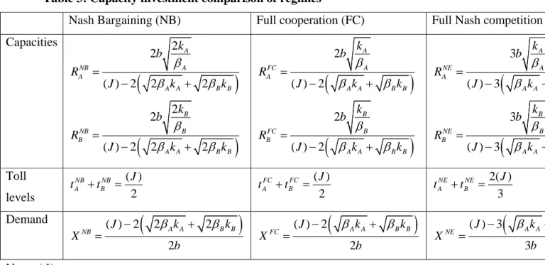
In Appendix 1 we derive the results under full cooperation and full Nash competition for this model, using the same procedure as in section 2.1. We summarize the results obtained for the three regimes considered in Tables 3 and 4. The rankings in Table 4 are based on the expressions in Table 3 after straightforward, but sometimes rather extensive, algebra.
Note that the rankings are the same as in the case of quality investment, except for the toll level. Therefore, bargaining yields more capacity, lower tolls, and both higher net toll revenues and more consumer benefits for road users than non-cooperative behavior.
Table 3: Capacity investment comparison of regimes
Nash Bargaining (NB) Full cooperation (FC) Full Nash competition Capacities
(
)
(
)
2 2 ( ) 2 2 2 2 2 ( ) 2 2 2 A A NB A A A B B B B NB B A A B B k b R J k k k b R J k k β β β β β β = − + = − +(
)
(
)
2 ( ) 2 2 ( ) 2 A A FC A A A B B B B FC B A A B B k b R J k k k b R J k k β β β β β β = − + = − +(
(
3 ( ) 3 3 ( ) 3 A A NE A A A B B NE B A A k b R J k k b R J k β β β β = − + = − + Toll levels ( ) 2 NB NB A B J t +t = ( ) 2 FC FC A B J t +t = 2( ) 3 NE NE A B J t +t = Demand ( ) 2(
2 2)
2 A A B B NB J k k X b β β − + = ( ) 2(
)
2 A A B B FC J k k X b β β − + = ( ) 3(
3 A A NE J k X b β − + = Note: ( )J = −a αA−αBTable 4: Comparison between regimes Comparison Nash bargaining (NB), full cooperation (FC) and Full Nash Competition (NE) Total toll per trip NE>FC=NB
Capacity FC>NB>NE
Demand (and congestion, and consumer surplus)
FC>NB>NE
3. Nash bargaining with a welfare maximizing government
In this section, we extend the model to allow for welfare maximizing governments. As our purpose is to point out the main differences with revenue maximizing behavior, we consider the simplest possible setup to illustrate the implications of taking into account the welfare of road users. Let us, therefore, interpret the two-region model as in Ubbels and Verhoef (2008). Region A is the city, region B is the surrounding region. Suppose all traffic in both A and B comes from commuters that travel from B to A. In such a setting is quite realistic to assume that region B cares about its commuting inhabitants. As there is no local traffic in the city, region A is assumed not to care about commuter welfare. So the respective welfare functions that we use are:
2 2 0 0.5 ( ) ( ) ( ) 0.5 ( ) A A A A X X X B B B B W t X m W p z dz g X X t X m γ γ = − ⎡ ⎤ =
∫
−⎣ ⎦ + − Here X( ) ( ) ( ) A A A A B B B Bg X =α +β X + m −t +α +β X + m −t is the total generalized cost (inclusive of toll payments) for a commuting trip. Demand is, as before, given by (4). We again consecutively consider quality and capacity investment (sections 3.1 and 3.2, respectively). To avoid too much repetition, we concentrate on the main differences with the previous section.
3.1. Maximizing welfare: toll and road quality choice under Nash bargaining
A. Nash bargaining
At the tolling stage, regions maximize joint welfare:
, ( , , , ) ( , , , )
A B
A A B A B B A B A B t t
Max W t t m m +W t t m m
Using the first-order conditions, it easily follows that the total tax to pass through the two regions equals the first best marginal external congestion cost:
( )
NB NB
A B A B
t +t = β +β X
[
]
2 2 NB NB A B A B A B A B A A t t a m m b β β α α β β + + = − − + + + + (29)Simple algebra shows that the toll level rises in quality and in the congestion functions’ slope parameters. Note that, for given quality levels, tolls are below those under revenue maximizing governments (compare with (6)). Optimal demand is
2 2 NB A B A B A B a m m X b α α β β − − + + = + +
Total welfare is, after substituting in the objective function:
2 2 2 ( ) ( , ) 0.5 0.5 ( ) 0.5 ( ) 2 2 A B A B A B A A B B A B a m m W m m m m b α α γ γ β β − − + + = − − + + (30)
The disagreement point is the Nash equilibrium in tolls. Country A solves:
[
]
2 ( , , , ) 0.5 ( ) A A A B A B A A t Max t X t t m m − γ mholding quality levels and toll levels in B constant. As before, the first-order conditions imply that region A charges, conditional on demand, more than marginal external cost:
1 2
( )
NE A
t = b+β β+ X . Similarly, region B solves:
2 0 ( ) ( ) 0.5 ( ) B X X X B B B t Max
∫
p z dz−⎡⎣g X ⎤⎦X +t X − γ mUsing the equilibrium condition that generalized price equals generalized cost, we easily show that the first order condition implies that region B charges exactly the ‘total’ marginal external cost, i.e., it charges for the congestion externality in both regions:
( )
NE
B A B
t = β +β X
The Nash equilibrium tolls are derived as in previous section. We find:
( ) 2 3 3 ( ) 2 3 3 NE A B A A B A B A B NE A B B A B A B A B b t a m m b t a m m b β β α α β β β β α α β β + + = − − + + + + + = − − + + + + (31)
Two points are worth noting. First, comparing with (9) we observe that, for given quality levels, region A charges more and region B charges less than in the case both regions
were maximizing toll revenues. Region B charges less because it cares for commuter welfare; region A charges more in response, given a negatively sloped reaction function. Second, tolls charged by A exceed those for region B: there is tax exporting by the city region A (also see De Borger et al. (2007), Ubbels and Verhoef (2008)).
Demand at the disagreement point is given by:
2 3 3 NE A B A B A B a m m X b α α β β − − + + = + + (32)
Using (31) and (32) in the respective objective functions, the welfare levels at the Nash disagreement point are shown to be, for given quality levels:
(
)
(
)
2 2 2 2 ( , ) ( ) 0.5 ( ) ( , ) 0.5 ( ) 0.5 ( ) NE NE A A B A B A A NE NE B A B A B B B W m m b X m W m m b X m β β γ β β γ = + + − = + + − (33)For equal quality cost parameters and quality levels, region A has a stronger pre-bargaining position. The reason is that, for given investment levels, it charges a higher toll than B and hence has larger revenues. Region B is weaker a priori because it wants a lower toll than A to account for commuter surplus. Interestingly, therefore, caring for consumers weakens region B’s pre-bargaining position.
The effect of more quality by region A on its bargaining position is given by:
(
)
2 ( ) 2 3 3 NE NE A B A B A B A A A A A B W W b a m m m m m b α α γ β β ∂ −∂ = − − + + − ∂ ∂ + +Offering more road quality raises A’s bargaining position if quality costs are low. In that case, more quality raises costs, but also increases demand, which raises revenues. Since A charges a higher toll than B the latter dominates if quality is not too costly. Similarly, we find for the effect of investment by B on its bargaining position:
(
)
2 ( ) 2 3 3 NE NE B A A B A B B B B B A B W W b a m m m m m b α α γ β β ∂ −∂ = − − − + + − ∂ ∂ + +Offering better road quality always reduces B’s bargaining position. It is costly and raises revenue more for region A than for B, weakening B’s position.
Finally, let us turn to the pre-bargaining quality investment game. Country A decides on quality by maximizing:
{
}
* 1 ( , ) ( , ) ( , ) ( , ) 2 NE NE A A B A B A A B B A B W m m = W m m +W m m −W m mThe first order condition for region A implies the following reaction function in quality:
(
)
2 ( ) 1 , 2 2 2 2 2 3 3 A B A A A B A A A A A A B A B a Z Z b m m Z Z Z b b α α γ γ β β β β − − = + = + − − + + + + (34)Reaction functions are upward sloping by the second-order conditions. A similar problem is solved by B. The corresponding reaction function is:
(
)
2 ( ) 1 , 2 2 2 2 2 3 3 A B B B B A B B B B B A B A B a Z Z b m m Z Z Z b b α α γ γ β β β β − − = + = − − − + + + + (35)Solving for the Nash equilibrium capacities yields:
( ) 2 ( ) 2 NB B A A B A A B B A A B NB A B A B B A B B A A B Z a m Z Z Z a m Z Z γ α α γ γ γ γ γ α α γ γ γ γ − − = − − − − = − − (36)
Note that, since ZA >ZBit follows that, assuming equal quality investment costs, the city region, interested in only its toll revenue, will actually invest more: NB NB
A B
m >m . The intuition is clear. If a region invests in more quality this is translated in more demand and hence higher tolls in both regions, but given the toll rules more so in A than B. The higher toll, however, reduces consumer surplus for commuters; hence, region B has an incentive to invest less in quality than A.
The bargaining position of A is captured by NE NE
A B
W −W , where both are evaluated at the bargaining quality outcomes. We find, using (36) in (33):
(
)
2(
)
2 2 2 ( ) 4 0.5 ( ) ( ) 2 2 3 3 NE NE A B A B A B A B A B B A A B A B B A A B a W W Z Z Z Z b γ γ α α γ γ γ γ γ γ γ γ β β ⎡ − − ⎤ ⎧⎪ ⎫⎪ − = ⎢ ⎥ ⎨ + − ⎬ − − + + ⎢ ⎥ ⎪ ⎪ ⎣ ⎦ ⎩ ⎭Note that this expression is always positive, unless the capacity cost parameter in B is very large. This makes sense: under ‘normal’ conditions A has a stronger bargaining position than B, as argued before. However, if the capacity cost in B is very high then B has a stronger position: it invests much less in quality, leading to lower demand but also lower tolls. Given the regions’ pricing policies this effect is more important for A than for B. Moreover, the toll reduction is appreciated by B because it raises consumer surplus of commuters. Both factors reduce the city region’s relative position.
2 ( ) 2 2 2 NB NB A B A B A B A B A A A B B A A A a t t b Z Z β β γ γ α α β β γ γ γ γ ⎡ ⎤ + − − + = ⎢ ⎥ + + ⎣ − − ⎦ (37) Demand is given by
[
2 2 (]
(
2) 2)
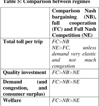
NB A B A B A B B A A B A A a X Z Z b γ γ α α γ γ γ γ β β − − = − − + + B. Comparison of regimesIn Appendix 2 we work out the analytics of full cooperation and full competition, and we provide details on the comparison of the results between the three regimes. The various comparisons of tolls, qualities, welfare levels, etc. are algebraically cumbersome, but the final results are quite similar to previous findings in Section 2. They are summarized in Table 5.
The main insight from this section is that bargaining partially resolves problems typically associated with tax and investment competition. The literature has shown that (see, e.g., De Borger, Dunkerley and Proost (2007) and Ubbels and Verhoef (2008)) Nash competition in both tolls and investment implies excessively high tolls and insufficient investment compared to the first best fully cooperative optimum, implying substantial welfare losses. We find that partial cooperation through Nash bargaining yields more investment, lower tolls and higher welfare than fully non-cooperative behavior. However, as regions use investment to affect their pre-bargaining position, welfare losses compared to the first-best do remain.
Table 5: Comparison between regimes Comparison Nash bargaining (NB), full cooperation (FC) and Full Nash Competition (NE) Total toll per trip FC>NB
NE>FC, unless demand very elastic and not much congestion
Quality investment FC>NB>NE Demand (and
congestion, and consumer surplus)
FC>NB>NE
Welfare FC>NB>NE
3.2. Maximizing welfare: toll and capacity investment under Nash bargaining
Finally, we considered a model with welfare maximizing regions and investment in road capacity. As before, generalized cost functions are:
1 ( ) ( ), , 1 ( ) ( ), , A A A A A A A A A A B B B B B B B B B B X C q q q XR R K K X C q q q XR R K K α β α β = + = = = = + = = =
We showed in Section 2 that the demand function for traffic is: ( , , , ) A B A B , A B A B A A B B a t t X t t R R N b R R N α α β β − − − − = = + +
The regions welfare functions can now be written as, respectively:
0 ( ) ( ) A A A A X X X B B B B k W t X R k W p z dz g X X t X R = − ⎡ ⎤ =
∫
−⎣ ⎦ + −The main difference with earlier analysis is that no closed-form solutions are available for optimal capacities, neither under bargaining nor under Nash competition. However, to the extent that analytical results can be derived, they are similar to those in
previous sections. This suggests that many of the results of previous sections are likely to carry over to this case, but that only numerical analysis can provide more information. We briefly go over the main steps of the analysis.
A. Nash bargaining
Nash bargaining: the tolling stage
Let the regions maximize joint welfare:
, 0 ( ) ( ) A B X X X A B A B A B t t A B k k Max W W p z dz g X X t X t X R R ⎡ ⎤ + =
∫
−⎣ ⎦ + + − −The first order conditions immediately imply the first-best toll regime:
( )
A B A A B B
t + =t β R +β R X
This amounts to charging the total marginal external cost of the commuting trip in both regions.
Using the demand function this can be rewritten as
[
]
( ) ( 2 2 ) A A B B A B A B A A B B R R t t a b R R β β α α β β + + = − − + +Unlike in case of revenue maximizing governments, the joint toll level now does depend on capacity provision. One easily shows that more capacity, since it reduces congestion, leads to lower tolls. Demand is, substituting toll levels:
( ) ( 2 2 ) NB A B A A B B a X b R R α α β β − − = + +
Total joint welfare equals, after substituting in the objective function:
2 ( ) 1 ( , ) 2 A B A B A B A A B B A B a k k W R R b R R R R α α β β ⎛ − − ⎞ = ⎜ ⎟− − + + ⎝ ⎠
Nash bargaining: the disagreement point
The disagreement point is the Nash equilibrium in tolls. Country A’s first order condition implies: