The Beta Workbench

(1)

Technical Report CoSBi 03/2007

The Beta Workbench

Alessandro Romanel

The Microsoft Research - University of Trento Centre for Computational and Systems Biology

DISI - Univerist`a di Trento romanel@cosbi.eu

Lorenzo Dematt´e

DISI - Univerist`a di Trento dematte@cosbi.eu

Corrado Priami

(2)

The Beta Workbench

Alessandro Romanel, Lorenzo Dematt´

e and Corrado Priami

The Microsoft Research - University of Trento

Centre for Computational and Systems Biology

{romanel,dematte,priami}@cosbi.eu

Abstract

This paper presents a system to model and simulate biological processes. It is based on process calculi theory and incorporates a language, a compiler, the execution environment and some graphical interface components. The language is based on 𝛽-binders, a recently introduced process algebra bio-inspired and developed to be suitable for the biological applicative domain. The runtime environment is based on a stochastic abstract machine that extends and improve the classical Gillespie’s approach. The quantitative aspects included in the stochastic information associated with the language allow to simulate and plot quantitative parameters of the system under investigation. We deﬁne the syntax, semantics and implementation of the language comparing our design choices with the most common features of pro-cess calculi applied to biology. A relevant part of this work is the de-scription of design patterns for the most common biological features in molecular interactions. This is an important aspect in exploiting the expressive power of the language and in providing a preliminary guide to the use of the compositional properties of process calculi.

(3)

1 Introduction

Biology is rapidly producing a huge number of experimental results and it is becoming impossible to coherently organize them using only human power. Abstract models to reason about biological systems is becoming an indispens-able conceptual and computational tool for biologists. An abstraction has to capture the essential properties of the phenomenon under consideration, and, at the same time, it has to be computable, to allow automatic analysis, and extensible, to permit the addition of further details [1]. Computer sci-ence modeling is speciﬁcally designed to meet the above requirements, but it heavily uses mathematical symbolism that is not easy to read for a neo-phyte. Therefore we need an approach that hides as many technical details as possible from users.

In recent times, a paradigmatic shift occurred in biology. Researchers started trying to build system visions rather than component visions, and the focus is now rapidly moving from structure to function. This process leads to the so-called Systems Biology [2] that is mostly interested in the behavior of cellular processes and in the description of the interactions among components. Seen from a computer science point of view, the methods and the techniques that could be best suited to face the challenge of systems biology are those related to the description and simulation of interacting distributed systems.

The process calculi approach to the formal modeling of biological systems has gained more and more attention over the last few years, particularly since the publication on Nature of the landmark paper by Regev and Shapiro [1]. Starting from the forerunner CCS, the ‘Calculus of Communicating Sys-tems’ [3], process calculi have been defined with the primary goal of providing formal specifications of concurrent processes, namely of computational enti-ties executing their tasks in parallel and able to synchronize over certain kinds of activities. The model of a system is typically given as a program or a term that defines the possible behaviors of the various components of the system. Calculi are then equipped with syntax-driven rules, the so-called operational semantics [4]. These rules, that can automatically allow the inference of the possible future of the system under analysis. For instance, they can specify that a certain process 𝑃 evolves into process 𝑄, written 𝑃 −→ 𝑄.

The basic entities of process calculi are actions and co-actions (comple-mentary actions). In the most basic view, like e.g. in CCS, an action is seen as an input or an output over a channel. Input is complementary to output and vice-versa. Actions and co-actions can also transmit/receive names over the channel (e.g. the IP address of the Internet) on which input and output are supposed to take place. This is, indeed, the underlying assumption taken

(6)

in the 𝜋-calculus [5]. As it will be clear in the rest of the paper, the actual interpretation of complementarity varies from one calculus to the other. The relevant fact to be pointed out here is that complementary actions are those that parallel processes can perform together to synchronize their (otherwise) independent behaviors.

Process calculi are typically very simple, yet contain all the ingredients for the description of concurrent systems in terms of what they can do rather than of what they are.

Two main properties of process calculi are worth mentioning. First, the meaning (behavior) of a complex system is expressed in terms of the meaning of its components. A model can be designed following a bottom-up approach: one defines the basic operations that a system can perform, then the whole behavior is obtained by composition of these basic building blocks. This property is called compositionality. Second, the mathematical rules defining the operational semantics of process calculi allow us to implement a simulator of the runs of the system. So process calculi are specification languages that can be directly implemented and executed.

The main contribution of this paper is the definition of a process-calculi based programming language designed to model biological systems. It is hence bio-inspired in the definition of the basic primitives. Furthermore we implemented the language providing quantitative tools that allow the user to model and simulate real case studies. We define first the syntax and the operational semantics of the calculus. Then we report some templates to model most of the common biological phenomena and we describe the software architecture of or implementation. Finally, we provide some hints on how to use the software components we developed.

2 Related work

In the last few years a number of process calculi have been adapted or newly developed for applications in systems biology. Some of the most important are:

∙ Biochemical stochastic calculus: is a stochastic extension of the 𝜋-calculus where biochemical interactions are represented as communica-tions of processes. Simulators for the Biochemical stochastic 𝜋-calculus [6] have been implemented, i.e. BioSpi1 and SPiM2 [7]. They are based on Gillespie’s assumption [8] and make in-silico experiments possible;

1

http://www.wisdom.weizmann.ac.il/ biospi/

2

(7)

∙ BioAmbients: is an extension of the Biochemical stochastic 𝜋-calculus where an explicit notion of compartments is introduced [9]. The lan-guage is provided with a stochastic extension and a simulator, based on Gillespies algorithm [10], has been implemented as part of the BioSpi project;

∙ Brane Calculus: is a calculus which is centered on membranes [11]. Brane calculus is inspired by BioAmbients, but it gives membranes an active role;

∙ Performance Evaluation Process Algebra (PEPA): is a formal language for describing Markov processes [12]. PEPA allows to quantitatively model and analyze large pathway systems. PEPA is supported by a large community and a lot of software tool for analysis and stochastic simulations are available.

∙ 𝜅-calculus: is a formal calculus of proteins interaction [13, 14]. It was designed to represent complexation and decomplexation of proteins. The 𝜅-calculus comes equipped with a very clear visual notation, and uses the concept of shared names to represents bonds.

For a more detailed introduction of process calculi and their application in biology, we refer the reader to [15].

3 The Language

The BetaSIM language is based on 𝛽-binders [16, 17], a process calculus developed for better representing the interactions between biological entities, and its stochastic extension. The main idea of 𝛽-binders is to encapsulate calculus processes into boxes with interaction capabilities. Like the 𝜋-calculus also 𝛽-binders is based on the notion of naming. Thus, we assume the existence of a countably infinite set 𝒩 of names (ranged over by lower-case letter) and a countably infinite set of interactions capabilities 𝒯 (ranged over by indexed 𝛿). We also assume a special name 𝜏 ∕∈ 𝒩 ∪ 𝒯 to express internal activities of processes or delays. BetaSIM has several modifications with respect to the original syntax and all of them will be discussed throughout the paper.

A BetaSIM program, called also 𝛽-system, is a tuple 𝑍=⟨𝐵, 𝐸, 𝜉⟩ which is a composition of a bio-process 𝐵, a list of events 𝐸 and environment 𝜉. The bio-process 𝐵 intuitively represents the structure of the system, that is a set of entities interacting in the same context, 𝐸 represents the list of possible

(8)

events enabled on the system and the environment 𝜉 contains information like the set T of considered types (ranged over by Δ, Γ0, Σ′, ⋅ ⋅ ⋅ ).

3.1 The syntax

In this section we describe the syntax of the bio-processes, of the events and the structure of the environment. We will also discuss the pi-processes 𝑃 .

The bio-process 𝐵 and the list of events 𝐸 are deﬁned according to the following context-free grammar:

𝐵 ::= Nil

∣

𝐵[𝑃 ]⃗

∣

𝐵∣∣𝐵 ⃗ 𝐵 ::= 𝛽(𝑥, 𝑟, Δ)ˆ

∣

𝛽(𝑥, 𝑟, Δ) ⃗ˆ 𝐵 ˆ 𝛽 ::= 𝛽

∣

𝛽ℎ

∣

𝛽𝑐 𝑃 ::= nil

∣

𝑃 ∣𝑃

∣

!𝜋.𝑃

∣

𝑀 𝑀 ::= 𝜋.𝑃

∣

𝑀 + 𝑀 𝜋 ::= 𝑥(𝑦)

∣

𝑥⟨𝑦⟩

∣

(𝜏, 𝑟)

∣

(die, 𝑟)

∣

(ch(𝑥, Δ), 𝑟)

∣

(hide(𝑥), 𝑟)

∣

(unhide(𝑥), 𝑟)

∣

(expose(𝑥, 𝑠, Δ), 𝑟) 𝑐𝑜𝑛𝑑 ::= 𝐵[𝑃 ] : 𝑟⃗

∣

∣ ⃗𝐵[𝑃 ]∣ = 𝑛

∣

𝐵[𝑃 ], ⃗⃗ 𝐵[𝑃 ] : 𝑟

𝑣𝑒𝑟𝑏 ::= new( ⃗𝐵[𝑃 ], 𝑛)

∣

split( ⃗𝐵[𝑃 ], ⃗𝐵[𝑃 ])

∣

join( ⃗𝐵[𝑃 ])

∣

delete 𝑒𝑣𝑒𝑛𝑡 ::= ∙

∣

(𝑐𝑜𝑛𝑑) 𝑣𝑒𝑟𝑏

𝐸 ::= 𝑒𝑣𝑒𝑛𝑡

∣

𝑒𝑣𝑒𝑛𝑡 :: 𝐸

where 𝑥, 𝑦 ∈ 𝒩 , 𝑛 ∈ ℕ and 𝑟 ∈ ℝ+∪ ∞ is a stochastic rate3_.

3.1.1 Bio-processes ad pi-processes

Bio-processes (or boxes) generated by the non terminal symbol 𝐵 can be either elementary bio-processes (the ﬁrst two productions) or a parallel com-position of elementary bio-processes, i.e. bio-processes running concurrently. The special process Nil does nothing; i.e. it is the deadlocked bio-process. The bio-process ⃗𝐵[𝑃 ] is a pi-process (see below) preﬁxed by a specialized beta binder ⃗𝐵 that represents the interaction capabilities of the bio-process. The intuition is that a bio-process represent a biological entity that has its own control mechanism (the pi-process 𝑃 ) and some interaction capabilities expressed by the beta binder.

A beta binder ⃗𝐵 is made up of a non empty list of elementary beta binders of the form 𝛽(𝑥, 𝑟, Γ) (active), 𝛽ℎ(𝑥, 𝑟, Γ) (hidden) or 𝛽𝑐(𝑥, 𝑟, Γ) (complexed ),

3_{A stochastic rate is the single parameter deﬁning an exponential distribution that}

drives the stochastic behaviour of an action. The rate ∞ is used to denote immediate actions, i.e., actions that are executed as soon as they become enabled.

(9)

where the name 𝑥 is the subject of the beta binder, 𝑟 is the stochastic pa-rameter that quantitatively drives the activities involving the binder and Γ represents the type of 𝑥. The subject 𝑥 of an elementary beta binder is a binding occurence that binds all the free occurrences of 𝑥 in the box to which the binder belongs. Hidden binders are useful to model interaction sites that are not available for interaction although their status can vary dynamically. For instance a receptor that is hidden by the shape of a molecule and that becomes available if the molecules interacts with/binds to other molecules. The complexed binders states that the corresponding box is physically bound through that interaction site to another box. We deﬁne three auxiliary func-tions to extract the set of subjects, the set of all types and the set of the complexed elementary beta binders from a beta binder.

With 𝒫, ℬℬ and ⃗ℬℬ we denote respectively the set of all the possible pi-processes, bio-processes and beta binder.

Deﬁnition 1. Let ⃗ℬℬ be the set of beta binders. Then, 𝑠𝑢𝑏 : ⃗ℬℬ → 2𝒩_;

𝑡𝑦𝑝𝑒𝑠 : ⃗ℬℬ → 2𝑇 _{and 𝑏𝑐 : ⃗}_{ℬℬ → 2}𝑇 _{are deﬁned as follows}

𝑠𝑢𝑏(𝛽(𝑥, 𝑟, Γ)) = 𝑠𝑢𝑏(𝛽ℎ_{(𝑥, 𝑟, Γ)) = 𝑠𝑢𝑏(𝛽}𝑐_{(𝑥, 𝑟, Γ)) = {𝑥}} 𝑠𝑢𝑏( ˆ𝛽(𝑥, 𝑟, Γ) ⃗𝐵) = {𝑥} ∪ 𝑠𝑢𝑏( ⃗𝐵) 𝑡𝑦𝑝𝑒𝑠(𝛽(𝑥, 𝑟, Γ)) = 𝑡𝑦𝑝𝑒𝑠(𝛽ℎ_{(𝑥, 𝑟, Γ)) = 𝑡𝑦𝑝𝑒𝑠(𝛽}𝑐_{(𝑥, 𝑟, Γ)) = {Γ}} 𝑡𝑦𝑝𝑒𝑠( ˆ𝛽(𝑥, 𝑟, Γ) ⃗𝐵) = {Γ} ∪ 𝑡𝑦𝑝𝑒𝑠( ⃗𝐵) 𝑏𝑐(𝛽(𝑥, 𝑟, Γ)) = 𝑏𝑐(𝛽ℎ(𝑥, 𝑟, Γ)) = ∅ 𝑏𝑐(𝛽𝑐_{(𝑥, 𝑟, Γ)) = {Γ}} 𝑏𝑐( ˆ𝛽(𝑥, 𝑟, Γ) ⃗𝐵) = 𝑏𝑐( ˆ𝛽(𝑥, 𝑟, Γ)) ∪ 𝑏𝑐( ⃗𝐵)

We now deﬁne well-formed bio-processes (assuming hereafter that the operator ∣ − ∣ denotes the cardinality of the argument, i.e. the length of a string, the length of a list or the number of elements of a set, letting the context disambiguate the overloaded symbol).

Deﬁnition 2. Let 𝐵 = ⃗𝐵1[𝑃1] ∣∣ ⋅ ⋅ ⋅ ∣∣ ⃗𝐵𝑛[𝑃𝑛] be a bio-process. We say that

𝐵 is well-formed if ∀𝑖 ∈ {1, ..., 𝑛}. ⃗𝐵𝑖 is well-formed.

A beta binder is well-formed if ∣ ⃗𝐵𝑖∣ = ∣𝑠𝑢𝑏( ⃗𝐵𝑖)∣ = ∣𝑡𝑦𝑝𝑒𝑠( ⃗𝐵𝑖)∣ > 0.

The condition on beta binders states that a well-formed beta binder is a non-empty string of elementary beta binders where subjects and types are all distinct.

Processes generated by the non terminal symbol 𝑃 are referred as pi-processes. The nil process does nothing; it is a deadlocked process. The

(10)

binary operator ∣ composes two processes that can run concurrently. The bang operator ! is used to replicate copies of the pi-process passed as argu-ment. Note that we use only guarded replication, i.e. the process argument of the ! must have a preﬁx 𝜋 that forbids any other action of the process until it has been consumed. The last non-terminal symbol 𝑀 of the productions of 𝑃 is used to introduce guarded choices. In fact 𝑀 generates summations of guarded preﬁxes of the form 𝜋.𝑃 .

The actions that a pi-process can perform are described by the syntactic category 𝜋. The first two actions are common to most process calculi. They represent respectively the input/reception of something that will instantiate the placeholder 𝑦 over a channel named 𝑥 (𝑥(𝑦)) and the output/send of a value 𝑦 over a channel named 𝑥 (𝑥⟨𝑦⟩). The placeholder 𝑦 in the input is a binding occurrence that binds all the free occurrences of 𝑦 in the scope of the prefix 𝑥(𝑦). Sometimes the channel name 𝑥 is called subject and the placeholder/value 𝑦 is called object of the prefix. The action (𝜏, 𝑟) denotes internal activities not involved in interactions of the pi-process that execute the prefix. Quantitatively, it is a delay driven by the stochastic parameter 𝑟. Parallel pi-processes that perform complementary actions on the same channel inside the same box (a process perform and input 𝑥(𝑧) and the other one an output 𝑥⟨𝑦⟩) can synchronize and exchange a message. The value 𝑦 flows from the process performing the output to the one performing the input. The flow of information affects the future behavior of the system because all the free occurrences of 𝑧 bound by the input placeholder are replaced in the receiving process by the actual value sent 𝑦. Pi-processes in different boxes can perform an inter-communication (distinct from the intra-communication described above) if one send out of the box a value 𝑦 over a link 𝑥 that is bound to an active binder of the box 𝛽(𝑥, 𝑟, Δ) and a pi-process in another box is willing to receive a value from a compatible binder 𝛽(𝑦, 𝑟, Γ) through the action 𝑦(𝑧). The two corresponding binders are compatible if a compatibility function 𝛼 applied to the types returns a real in ℝ+∪ ∞. Note that intra-communications occur on perfectly symmetric input/output pairs that share the same subject, while inter-communication can occur between primitives that has different subjects provided that their types are compatible. This new notion of communication is particularly relevant in biology interactions occur on the basis of affinity which can never be exact complementary of molecular structures. The same substance can interact with many other in the same context, although with different levels of affinity.

The remain actions are peculiar of the BetaSIM language. The action (die, 𝑟) destroy the box enclosing the pi-process that executes the preﬁx. The action (ch(𝑥, Δ), 𝑟) change the type of the binder with subject 𝑥 to Δ. The

(11)

actions (hide(𝑥), 𝑟) and (unhide(𝑥), 𝑟) are complementary and they change the state of an active binder to hidden and vice versa. Finally, the action (expose(𝑥, 𝑠, Δ), 𝑟) creates a new binder for the current box with subject 𝑥, rate 𝑠 and type Δ. The subject 𝑥 of the newly created binder is a binding occurrence that binds all the free occurrence of 𝑥 in the preﬁxed pi-process.

3.1.2 Events

The non terminal symbol E generates a list of events. A list of events is always related to a bio-process B and each single event occurs only if its condition is satisﬁed on a set of one or more boxes composing B. A single event is the composition of a condition cond and an action verb and is a riformulation of the 𝑓𝑗𝑜𝑖𝑛and 𝑓𝑠𝑝𝑙𝑖𝑡axioms of the original 𝛽-binders deﬁnition.

To gain eﬃciency with respect to 𝛽-binders, in the present version of the language conditions are limited to structural congruence of bio-processes and cardinality of the equivalence classes originated by the structural congruence (more detail will be available in Subsect. ??). In particular, given a bio-process 𝐵, the condition ⃗𝐵[𝑃 ] : 𝑟 (∣ ⃗𝐵[𝑃 ]∣ = 𝑛) is satisﬁed if there is at least one (exactly 𝑛) box in B that is equivalent4 _{to ⃗}_{𝐵[𝑃 ]. The condition}

⃗

𝐵[𝑃 ], ⃗𝐵[𝑃 ] : 𝑟 is satisﬁed if B contains at least a bio-process equivalent to the ﬁrst element of the pair and at least a bio-process equivalent to the second element of the pair. The stochastic information associated to conditions will be described in the next subsection.

The syntactic category 𝑣𝑒𝑟𝑏 denotes the actions that are associated with conditions. The action new( ⃗𝐵[𝑃 ], 𝑛) creates 𝑛 new instances of the bio-process speciﬁed as argument. Hereafter when the created bio-bio-process coin-cides with the one speciﬁed in the condition we will write for short new(𝑛). The action split( ⃗𝐵[𝑃 ], ⃗𝐵[𝑃 ]) remove a copy of the box in the condition and introduces the two processes arguments of the split operation. The action join( ⃗𝐵[𝑃 ]) remove a copy of each of the bio-processes in the condition and introduce a copy of its argument. Finally, the action delete remove a copy of the bio-process in the condition.

The action new can be used to model, for example, the translation of new proteins and enzymes in the cell at a given rate, or the introduction of a new bio-process from the external environment (entrance of hormones, nutrients or other entities in the cell) without necessarly modelling the whole transport or synthesis pathway. The actions split and join can represent

4_{We are using the word equivalent here to mean structurally congruent. Since this}

concept is introduced later in the paper we remain vague deliberately relying on the intuition.

(12)

classical bind/unbind reactions in molecular environments. Finally delete is useful to model the decay or degradation of entities (such as molecules and proteins).

We now deﬁne well-formed events.

Deﬁnition 3. Let (cond) verb be an event. We say that the event is well-formed if it satisﬁes one of the following forms and conditions:

- ( ⃗𝐵1[𝑃1] : 𝑟) split( ⃗𝐵2[𝑃2], ⃗𝐵3[𝑃3])

with (𝑏𝑐( ⃗𝐵2) ∩ 𝑏𝑐( ⃗𝐵3) = ∅) and (𝑏𝑐( ⃗𝐵2) ∪ 𝑏𝑐( ⃗𝐵3) = 𝑏𝑐( ⃗𝐵1));

- ( ⃗𝐵1[𝑃1], ⃗𝐵2[𝑃2] : 𝑟) join( ⃗𝐵3[𝑃3])

with ((𝑏𝑐( ⃗𝐵1) ∩ 𝑏𝑐( ⃗𝐵2) = ∅) and (𝑏𝑐( ⃗𝐵1) ∪ 𝑏𝑐( ⃗𝐵2) = 𝑏𝑐( ⃗𝐵3));

- ( ⃗𝐵[𝑃 ] : 𝑟) new( ⃗𝐵′[𝑃′], 𝑛) with 𝑏𝑐( ⃗𝐵) = ∅;

- (∣ ⃗𝐵[𝑃 ]∣ = 𝑚) new( ⃗𝐵′[𝑃′], 𝑛) with 𝑏𝑐( ⃗𝐵) = ∅ and ⃗𝐵′[𝑃′] ≡𝑏 𝐵[𝑃 ];⃗

- ( ⃗𝐵[𝑃 ] : 𝑟) delete with 𝑏𝑐( ⃗𝐵) = ∅.

A list 𝐸 of events is well-formed if all its events are well-formed.

The intuition underlying the above deﬁnition is that manipulation of boxes must take care of complexes. In particular, it is forbidden to create new copies or to destroy boxes that are part of complexes (last three items).

3.1.3 Graphical syntax

The BetaSIM language is also provided with a graphical representation of boxes:

𝑃

(𝑥1: Δ1)𝑟 (𝑥2: Δ2)ℎ𝑟 (𝑥3 : Δ3)𝑟

The pairs 𝑥𝑖 : Δ𝑖 represent the sites through which the box may interact

with other boxes. Types Δ𝑖 express the interaction capabilities at 𝑥𝑖. The

value 𝑟 represent the stochastic rate, ℎ represents the hidden status and the black line over the last beta binder represents the complexed status. 𝑃 is the pi-process deﬁning the internal structure of the box. Hereafter, we assume that all the boxes around are composed in a 𝛽-system through the ∣∣ operator.

3.1.4 The environment

The environment 𝜉 contains the set 𝑇 of types, the aﬃnity function 𝛼 : 𝑇2 _{→ ℝ}3_{, the function 𝜌 : 𝒩 → ℝ and a symmetric binary relation ⊙, called} complexation relation.

(13)

In the original paper of 𝛽-binders, types are defined over sets of names in 𝒩 . However, we refer to a more general definition of type. In particular, we assume that the elements composing 𝑇 are defined over algebric structures with decidable equality relation.

The function 𝛼 is the aﬃnity function. Given two types Δ and Γ, the application 𝛼(Δ, Γ)=(𝑟, 𝑠, 𝑡) returns a measure of the compatibility of the two types. The value 𝑟 represents the complexation stochastic rate, the value 𝑠 represents the decomplexation stochastic rate and 𝑡 represents the inter-communication stochastic rate. In the next sections the meant of com-plexation and decomcom-plexation will be clearily explained.

We deﬁne also three auxiliary 𝛼𝑐(Δ, Γ) = 𝑟, 𝛼𝑑(Δ, Γ) = 𝑠 and 𝛼𝑖(Δ, Γ) =

𝑡 that project the components of the result of 𝛼(Δ, Γ).

The function 𝜌 associates stochastic rates to names in 𝒩 . Given 𝜌(𝑥)=𝑟, the value 𝑟 drives the stochastic behaviour of the communications enabled on the channel 𝑥.

Deﬁnition 4. Let ℒ = {∥0, ∥1} and 𝜗 ∈ ℒ∗. The set of labels 𝐿 (with

metavariable 𝛾) is deﬁned as 𝛾 ::= 𝜗Δ, where Δ ∈ 𝑇 .

Labels 𝜗 are also called localities and are used to provide interaction sites of boxes with unique names. The complexation relation ⊙ ⊆ 𝐿 × 𝐿 is a symmetric binary relation deﬁned over the set of labels Θ. Intuitively, ⊙ states that two interaction sites are joined in a complex. We say that the relation ⊙ is well-formed if for each pair (𝛾, 𝛾′) ∈ ⊙ there does not exist another pair in ⊙ that contains 𝛾 or 𝛾′.

Deﬁnition 5. Let ⊙ be a complexation relation. The relation ⊙ is well-formed if 𝛾 ⊙ 𝛾′∧ 𝛾 ⊙ 𝛾′′ _{⇒ 𝛾}′ _{= 𝛾}′′_.

Two labels are connected if there exists a path of relations built by ⊙ that relates the two labels, i.e., the corresponding interaction sites are part of the same complex.

Deﬁnition 6. Let ⊙ be a well-formed complexation relation and let 𝛾, 𝛾′ ∈ ⊙. Then 𝛾 and 𝛾′ _{are connected, denoted with 𝛾⊙𝛾}′_{, if there exists labels}

𝛾1 = 𝜗1Δ1, ⋅ ⋅ ⋅ , 𝛾𝑛 = 𝜗𝑛Δ𝑛 such that

(𝛾 = 𝛾1) ∧ (𝛾′ = 𝛾𝑛) ∧ (∀𝑖 ∈ {1, ..., 𝑛/2}𝛾2𝑖−1⊙ 𝛾2𝑖)∧

(∀𝑖 ∈ {1, ..., (𝑛/2) − 1}(𝜗2𝑖 = 𝜗2𝑖+1∧ Δ2𝑖∕= Δ2𝑖+1))

Since ⊙ is well-formed, then we are sure that the value 𝑛 is even. We also introduce a notion of substitution of environment elements. In particular, given an environment 𝜉 = (𝑇, 𝛼, 𝜌, ⊙) and element 𝑇′, 𝛼′, 𝜌′ and ⊙′, a sub-stitution is deﬁned in the following way:

(14)

𝜉[𝑇′] = (𝑇′, 𝛼, 𝜌, ⊙) 𝜉[𝛼′] = (𝑇, 𝛼′, 𝜌, ⊙) 𝜉[𝜌′] = (𝑇, 𝛼, 𝜌′, ⊙) 𝜉[⊙′] = (𝑇, 𝛼, 𝜌, ⊙′) Sequential substitution are possible,

𝜉[𝑇′][𝛼′][𝜌′][⊙′] = (𝑇′, 𝛼′, 𝜌′, ⊙′)

Moreover, with 𝑇𝜉, 𝛼𝜉, 𝜌𝜉and ⊙𝜉we indicate the elements of the environment

𝜉.

3.2 The operational semantics

The evolution of the system is formally specified through the operational semantics of the language, which is defined with a limited number of oper-ations. In order to define the semantics, we first enrich the language with labels that allow us to identify in a unique way all the boxes composing the considered system.

We use the localities 𝜗, previously introduced, and we use them to label boxes. We then replace each box ⃗𝐵[𝑃 ] with a labeled box 𝜗 ⃗𝐵[𝑃 ] (where 𝜗 provides a linear encoding of the syntactical location of the box ⃗𝐵[𝑃 ] in the syntax tree of the whole initial system).

For instance, the bio-process 𝛽ℎ(𝑥, 𝑟, Δ)[𝑃 ] ∥ 𝛽(𝑧, 𝑠, Σ)[𝑄] is mapped to the bio-process (∥0 𝛽ℎ(𝑥, 𝑟, Δ)[𝑃 ]) ∥ (∥1 𝛽(𝑧, 𝑠, Σ)[𝑄]). Graphically, such a

parallel composition of bio-processes can be represented in the following way:

∥0 𝑥(𝑚).𝑃

∣

𝑥⟨𝑧⟩.𝑄

(𝑥 : Δ)𝑟

∥1 𝑃 {𝑧/𝑚}

∣

𝑄

(𝑥 : Δ)𝑟

where the labels that precede the boxes are the localities associated to them. For semplicity, if parallel boxes 𝜗𝐵[𝑃 ] ∥ 𝜗′′𝐵′[𝑃′] have labels 𝜗 = 𝜗0𝜗1

𝜗′ = 𝜗0𝜗2 that share subparts, than it is possible to represent the bio-process

also with 𝜗0(𝜗1𝐵[𝑃 ] ∥ 𝜗2𝐵′[𝑃′]).

In the reminder of the technical report, when not necessary, we will omit the localities, either in the formal and graphical representation. Moreover, the operational semantics of the language is deﬁned up to structural con-gruence. The structural congruence for the BetaSIM 𝛽-systems is deﬁned through a structural congruence over pi-processes, a structural congruence over beta-processes and a structural congruence over events.

(15)

Deﬁnition 7. The structural congruence over pi-processes, denoted ≡𝑝, is

the smallest relation which satisﬁes the laws in Fig. 1 (group a), the structural congruence over beta-processes, denoted ≡𝑏, is the smallest relation which

sat-isﬁes the laws in Fig. 1 (group b) and the structural congruence over events, denoted ≡𝑒, is the smallest relation which satisﬁes the laws in Fig. 1 (group

c).

Hence, two 𝛽-systems 𝑍 = ⟨𝐵, 𝐸, 𝜉⟩ and 𝑍′ = ⟨𝐵′, 𝐸′, 𝜉′⟩ are structurally congruent, indicated with 𝑍 ≡ 𝑍′, only if 𝐵 ≡𝑏 𝐵′, 𝐸 ≡𝑒𝐸′ and 𝜉 = 𝜉′.

Notice that the structural congruence do not consider the presence of locations associated to boxes. In general, considering also the locations, we have to guarantee that they do not change under structural congruence. Formally, assuming 𝐵 and 𝐵′ bio-processes, we have that:

𝜗𝐵 ≡𝑏 𝜗′𝐵′ ⇔ 𝜗 = 𝜗′∧ 𝐵 ≡𝑏 𝐵′

The structural congruence is computable and hence we can eﬀectively implement it.

Theorem 1. The relation ≡ is decidable.

Proof. We report here a sketch of the proof. The set of bio-processes ℬℬ match with the set ℬℬ𝑒, introduced in [18]. Therefore the structural congruence ≡𝑏 is

decidable and efficently solvable. As a consequence, also the structural congruece ≡_𝑒is efficently solvable and therefore the structural congruence ≡ is decidable and efficently solvable. More details are in [18].

The operational semantics of the language is deﬁned using a reduction relation →𝑠, which uses a labeled reduction relation

𝜃

− → .

Deﬁnition 8. The set of labels Θ, with metavariable 𝜃, is deﬁned in the following way:

𝜃 ::= 𝑟, 𝑡𝑦𝑝𝑒, 𝑑𝑎𝑡𝑎

where 𝑟 ∈ ℝ, 𝑡𝑦𝑝𝑒 ∈ {𝑑𝑖𝑒, 𝑛𝑒𝑤} and 𝑑𝑎𝑡𝑎 is a generic string. The function 𝑟𝑎𝑡𝑒 : Θ → ℝ returns the value r of the triple.

The main concept of 𝛽-binders is to encapsulate of processes into boxes with interaction capabilities. This encapsulation allows us to distinguish between three types of operations: monomolecular, bimolecular and events. Monomolecular operations describe the evolution of single entities and there-fore we deﬁne them intra actions; the other two kinds of operations describe interactions that involves two or more entities, and so they are deﬁned inter actions.

(16)

group a - 𝑃1 ≡𝑝 𝑃2 if 𝑃1 and 𝑃2 𝛼-equivalent - 𝑃1 ∣ (𝑃2 ∣ 𝑃3) ≡𝑝 (𝑃1 ∣ 𝑃2) ∣ 𝑃3 - 𝑃1 ∣ 𝑃2 ≡𝑝 𝑃2 ∣ 𝑃1 - 𝑃 ∣ nil ≡𝑝 𝑃 - 𝑀1+ (𝑀2+ 𝑀3) ≡𝑝 (𝑀1+ 𝑀2) + 𝑀3 - 𝑀1+ 𝑀2 ≡𝑝𝑀2+ 𝑀1 - !𝜋.𝑃 ≡𝑝𝜋.(𝑃 ∣ !𝜋.𝑃 ) group b - ⃗𝐵[𝑃1] ≡𝑏𝐵[𝑃⃗ 2] if 𝑃1 ≡ 𝑃2 - 𝐵1 ∣∣ (𝐵2 ∣∣ 𝐵3) ≡𝑏 (𝐵1 ∣∣ 𝐵2) ∣∣ 𝐵3 - 𝐵1 ∣∣ 𝐵2 ≡𝑏 𝐵2 ∣∣ 𝐵1 - 𝐵 ∣∣ Nil ≡𝑏 𝐵 - ⃗𝐵1𝐵⃗2[𝑃 ] ≡𝑏𝐵⃗2𝐵⃗1[𝑃 ] - ⃗𝐵∗𝛽(𝑥, 𝑟, Γ)[𝑃 ] ≡ˆ _𝑏 𝐵⃗∗𝛽(𝑦, 𝑟, Γ)[𝑃 {𝑦/𝑥}]ˆ with 𝑦 fresh in 𝑃 and 𝑦 ∕∈ 𝑠𝑢𝑏( ⃗𝐵∗) group c - (𝐵0 : 𝑟) 𝑠𝑝𝑙𝑖𝑡(𝐵1, 𝐵2) ≡𝑒(𝐵′0: 𝑟) 𝑠𝑝𝑙𝑖𝑡(𝐵1′, 𝐵2′) if 𝐵0≡𝑏 𝐵0′, 𝐵1≡𝑏 𝐵1′ and 𝐵2 ≡𝑏 𝐵′2 - (𝐵 : 𝑟) 𝑑𝑒𝑙𝑒𝑡𝑒 ≡𝑒(𝐵′ : 𝑟) 𝑑𝑒𝑙𝑒𝑡𝑒, if 𝐵 ≡𝑏 𝐵′ - (𝐵 : 𝑟) 𝑛𝑒𝑤(𝐵1, 𝑛) ≡𝑒(𝐵′ : 𝑟) 𝑛𝑒𝑤(𝐵1′, 𝑛) if 𝐵 ≡𝑏 𝐵′ and 𝐵1≡𝑏 𝐵1′ - (∣𝐵∣ = 𝑚) 𝑛𝑒𝑤(𝐵1, 𝑛) ≡𝑒 (∣𝐵′∣ = 𝑚) 𝑛𝑒𝑤(𝐵1′, 𝑛) if 𝐵 ≡𝑏 𝐵′ and 𝐵1≡𝑏 𝐵1′ - (𝐵0, 𝐵1 : 𝑟) 𝑗𝑜𝑖𝑛(𝐵2) ≡𝑒(𝐵0′, 𝐵1′ : 𝑟) 𝑗𝑜𝑖𝑛(𝐵2′) if 𝐵0≡𝑏 𝐵0′, 𝐵1≡𝑏 𝐵1′ and 𝐵2 ≡𝑏 𝐵′2 - 𝐸0::𝐸1 ≡𝑒 𝐸1::𝐸0

Figure 1: Structural laws for BetaSIM language.

3.2.1 Monomolecular operations

The formal semanctics of monomoecular operations is reported in Table 1. Hereafter substitutions are typed as {−/−} : 𝒩 → 𝒩 . In general, intra-boxes communication allows components within the same box to interact,

𝑥(𝑚).𝑃

∣

𝑥⟨𝑧⟩.𝑄

(𝑥 : Δ)𝑟

→ 𝑃 {𝑧/𝑚}

∣

𝑄

(17)

The expose action adds a new site of interaction to the interface, the change action modiﬁes the type of an interaction site,

(expose(𝑥, 𝑠, Σ), 𝑟).𝑃 (𝑥 : Δ)𝑟 → (ch(𝑦, Γ), 𝑟).𝑛𝑖𝑙 (𝑥 : Δ)𝑟 (𝑦 : Σ)𝑠 → 𝑛𝑖𝑙 (𝑥 : Δ)𝑟 (𝑦 : Γ)𝑠

the hide and unhide actions makes respectively invisible and visible an interaction site. (hide(𝑥), 𝑟).𝑃 (𝑥 : Δ)𝑟 → (unhide(𝑦), 𝑟).𝑛𝑖𝑙 (𝑥 : Δ)ℎ_𝑟 → 𝑛𝑖𝑙 (𝑥 : Δ)𝑟

and the die action eliminates the box that performs the action and, by propa-gating the proper information with the label 𝜃 = 𝑟, 𝑑𝑖𝑒, 𝜗 through the deriva-tion tree, cause the eliminaderiva-tion of all the boxes directly or indirectly com-plexed with them. In the Sect. 5, this mechanism will be clearily explained. Notice that the environment is modiﬁed to delete all the bindings in which the eliminated box is involved.

(intra) ⟨𝜗 ⃗𝐵[𝑥⟨𝑧⟩. 𝑃1+ 𝑀1∣ 𝑥(𝑤). 𝑃2+ 𝑀2∣ 𝑃3], 𝐸, 𝜉⟩ 𝜌(𝑥),∙,𝜖 −−−−−→ ⟨𝜗 ⃗𝐵[𝑃1∣ 𝑃2{𝑧/𝑤} ∣ 𝑃3], 𝐸, 𝜉⟩ (tau) ⟨𝜗 ⃗𝐵[(𝜏, 𝑟). 𝑃1+ 𝑀1∣ 𝑃2], 𝐸, 𝜉⟩ 𝑟,∙,𝜖 −−−→ ⟨𝜗 ⃗𝐵[𝑃1∣ 𝑃2], 𝐸, 𝜉⟩ (expose) ⟨𝜗 ⃗𝐵[(expose(𝑥, 𝑠, Γ), 𝑟). 𝑅 + 𝑀 ∣ 𝑄], 𝐸, 𝜉⟩−−−→ ⟨𝜗 ⃗𝑟,∙,𝜖 𝐵 𝛽(𝑦, 𝑠, Γ)[𝑅{𝑦/𝑥} ∣ 𝑄], 𝐸, 𝜉⟩ 𝑦 ∕∈ 𝑠𝑢𝑏( ⃗𝐵) 𝑎𝑛𝑑 Γ ∕∈ 𝑡𝑦𝑝𝑒𝑠( ⃗𝐵) (change) ⟨𝜗 ⃗𝐵∗𝛽(𝑥, 𝑠, Δ)[(ch(𝑥, Γ), 𝑟). 𝑅 + 𝑀 ∣ 𝑄], 𝐸, 𝜉⟩−−−→ ⟨𝜗 ⃗𝑟,∙,𝜖 𝐵∗𝛽(𝑥, 𝑠, Γ)[𝑅 ∣ 𝑄], 𝐸, 𝜉⟩ (hide) ⟨𝜗 ⃗𝐵∗𝛽(𝑥, 𝑠, Δ)[(hide(𝑥), 𝑟). 𝑅 + 𝑀 ∣ 𝑄], 𝐸, 𝜉⟩−−−→ ⟨𝜗 ⃗𝑟,∙,𝜖 𝐵∗𝛽(𝑥, 𝑠, Δ)[𝑅 ∣ 𝑄], 𝐸, 𝜉⟩ (unhide) ⟨𝜗 ⃗𝐵∗𝛽ℎ_{(𝑥, 𝑠, Δ)[(unhide(𝑥), 𝑟). 𝑅 + 𝑀 ∣ 𝑄], 𝐸, 𝜉⟩}_{−−−→ ⟨𝜗 ⃗}𝑟,∙,𝜖 _𝐵∗_{𝛽(𝑥, 𝑠, Δ)[𝑅 ∣ 𝑄], 𝐸, 𝜉⟩}

(die) ⟨𝜗 ⃗𝐵[(die, 𝑟). 𝑅 + 𝑀 ∣ 𝑄], 𝐸, 𝜉⟩−−−−−→ ⟨Nil, 𝐸, 𝜉[⊙𝑟,𝑑𝑖𝑒,𝜗 ′_]⟩

where ⊙′= ⊙𝜉∖ {(𝜗0Δ, 𝜗1Γ) : 𝜗0= 𝜗 ∨ 𝜗1= 𝜗}

Table 1: Monomolecular reduction rules

3.2.2 Bimolecular operations

Bimolecular operations describe interactions that involves two boxes. The formal semantics of these operations is reported in Table 2.

Inter-communication represent the classical notion of communication be-tween boxes:

(18)

𝑥(𝑚).𝑃 (𝑥 : Δ)𝑟 𝑦⟨𝑧⟩.𝑄 (𝑦 : Γ)𝑟 → 𝑃 {𝑧/𝑚} (𝑥 : Δ)𝑟 𝑄 (𝑦 : Γ)𝑟

In particular, the communication is enabled only if the aﬃnity of the types of the involved elementary beta binders 𝛼(Δ, Γ) is a triple (0, 0, 𝑛) with 𝑛 > 0. This means that the complexation and decomplexation feature is not enabled and hence only a notion of communication is permitted. This also allows to maintain a compatibility with respect to the original version of 𝛽-binders, where complexation and decomplexation are not available.

Complex and decomplex operations create and delete dedicated communi-cation binding between boxes. The biological counterpart of this construct is the binding of a ligand to a receptor, or of an enzyme to a substrate through an active domain. Assume 𝛼(Δ, Γ) = (𝑟, 𝑠, 𝑡) with 𝑟, 𝑠, 𝑡 > 0. The complex operation creates, with rate 𝛼𝑐(Δ, Γ), a dedicated communication binding:

𝑃 (𝑥 : Δ)𝑟 𝑄 (𝑦 : Γ)𝑟 → 𝑃 (𝑥 : Δ)𝑟 𝑄 (𝑦 : Γ)𝑟

while the decomplex operation deletes, with rate 𝛼𝑑(Δ, Γ), an already

exist-ing bindexist-ing: 𝑃 (𝑥 : Δ)𝑟 𝑄 (𝑦 : Γ)𝑟 → 𝑃 (𝑥 : Δ)𝑟 𝑄 (𝑦 : Γ)𝑟

Notice that the information of the bindings is not present in the formal description of the boxes. What we know by the bio-process is that the el-ementary beta binders are in the complex status. For example, considering the graphical representation of the following bio-process:

𝜗𝑝 𝑃 (𝑥 : Δ)𝑟 𝜗𝑞 𝑄 (𝑦 : Γ)𝑟 𝜗𝑟 𝑅 (𝑥 : Δ)𝑟 𝜗𝑠 𝑆 (𝑦 : Γ)𝑟

with 𝜗𝑝 ∕= 𝜗𝑞 ∕= 𝜗𝑟 ∕= 𝜗𝑠, we do not know which box is complexed with which

other box. The information about the complexation is maintained by the symmetric binary relation ⊙𝜉 of the environment 𝜉. Several conﬁgurations

(19)

𝜗𝑝 𝑃 (𝑥 : Δ)𝑟 𝜗𝑞 𝑄 (𝑦 : Γ)𝑟 𝜗𝑟 𝑅 (𝑥 : Δ)𝑟 𝜗𝑠 𝑆 (𝑦 : Γ)𝑟 𝜗𝑝 𝑃 (𝑥 : Δ)𝑟 𝜗𝑞 𝑄 (𝑦 : Γ)𝑟 𝜗𝑟 𝑅 (𝑥 : Δ)𝑟 𝜗𝑠 𝑆 (𝑦 : Γ)𝑟

For the ﬁrst example it is

⊙𝜉= {(𝜗𝑝Δ, 𝜗𝑞Γ), (𝜗𝑟Δ, 𝜗𝑠Γ), (𝜗𝑞Γ, 𝜗𝑝Δ), (𝜗𝑠Γ, 𝜗𝑟Δ)}

while for the second example it is

⊙𝜉= {(𝜗𝑝Δ, 𝜗𝑠Γ), (𝜗𝑞Γ, 𝜗𝑟Δ), (𝜗𝑠Γ, 𝜗𝑝Δ), (𝜗𝑟Δ, 𝜗𝑞Γ)}

The well-formedness of the relation ⊙𝜉 preserves by situations in which

el-ementary beta binders are complexed with more than one other elel-ementary beta binders. For example, in the following conﬁguration:

𝜗𝑝 𝑃 (𝑥 : Δ)𝑟 𝜗𝑞 𝑄 (𝑦 : Γ)𝑟 𝜗𝑟 𝑅 (𝑥 : Δ)𝑟 𝜗𝑠 𝑆 (𝑦 : Γ)𝑟 ⊙𝜉 = {(𝜗𝑝Δ, 𝜗𝑞Γ), (𝜗𝑟Δ, 𝜗𝑠Γ), (𝜗𝑞Γ, 𝜗𝑝Δ), (𝜗𝑠Γ, 𝜗𝑟Δ), (𝜗𝑞Γ, 𝜗𝑟Δ),

(𝜗𝑟Δ, 𝜗𝑞Γ)} and the well-formedness condition is not preserved because there

exists pairs (𝜗𝑞Γ, 𝜗𝑝Δ) and (𝜗𝑞Γ, 𝜗𝑟Δ) such that 𝜗𝑟Δ ∕= 𝜗𝑝Δ.

Finally, the 𝑖𝑛𝑡𝑒𝑟-𝑐𝑜𝑚𝑝𝑙𝑒𝑥 operation enables, with rate 𝛼𝑖(Δ, Γ), a

com-munication between complexed boxes through the complexed elementary beta-binders: 𝑥(𝑚).𝑃 (𝑥 : Δ)𝑟 𝑦⟨𝑧⟩.𝑄 (𝑦 : Γ)𝑟 → 𝑃 {𝑧/𝑚} (𝑥 : Δ)𝑟 𝑄 (𝑦 : Γ)𝑟

A more intuitive discussion of 𝑐𝑜𝑚𝑝𝑙𝑒𝑥, 𝑑𝑒𝑐𝑜𝑚𝑝𝑙𝑒𝑥 and 𝑖𝑛𝑡𝑒𝑟-𝑐𝑜𝑚𝑝𝑙𝑒𝑥 operations is reported in Sect. 5.

(20)

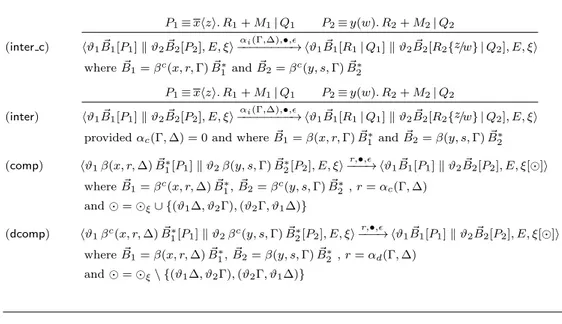
(inter c) 𝑃1≡ 𝑥⟨𝑧⟩. 𝑅1+ 𝑀1∣ 𝑄1 𝑃2≡ 𝑦(𝑤). 𝑅2+ 𝑀2∣ 𝑄2 ⟨𝜗1𝐵⃗1[𝑃1] ∥ 𝜗2𝐵⃗2[𝑃2], 𝐸, 𝜉⟩ 𝛼𝑖(Γ,Δ),∙,𝜖 −−−−−−−−→ ⟨𝜗1𝐵⃗1[𝑅1∣ 𝑄1] ∥ 𝜗2𝐵⃗2[𝑅2{𝑧/𝑤} ∣ 𝑄2], 𝐸, 𝜉⟩ where ⃗𝐵1= 𝛽𝑐(𝑥, 𝑟, Γ) ⃗𝐵∗1 and ⃗𝐵2= 𝛽𝑐(𝑦, 𝑠, Γ) ⃗𝐵2∗ (inter) 𝑃1≡ 𝑥⟨𝑧⟩. 𝑅1+ 𝑀1∣ 𝑄1 𝑃2≡ 𝑦(𝑤). 𝑅2+ 𝑀2∣ 𝑄2 ⟨𝜗1𝐵⃗1[𝑃1] ∥ 𝜗2𝐵⃗2[𝑃2], 𝐸, 𝜉⟩ 𝛼𝑖(Γ,Δ),∙,𝜖 −−−−−−−−→ ⟨𝜗1𝐵⃗1[𝑅1∣ 𝑄1] ∥ 𝜗2𝐵⃗2[𝑅2{𝑧/𝑤} ∣ 𝑄2], 𝐸, 𝜉⟩

provided 𝛼𝑐(Γ, Δ) = 0 and where ⃗𝐵1= 𝛽(𝑥, 𝑟, Γ) ⃗𝐵1∗and ⃗𝐵2= 𝛽(𝑦, 𝑠, Γ) ⃗𝐵2∗

(comp) ⟨𝜗1𝛽(𝑥, 𝑟, Δ) ⃗𝐵∗1[𝑃1] ∥ 𝜗2𝛽(𝑦, 𝑠, Γ) ⃗𝐵2∗[𝑃2], 𝐸, 𝜉⟩ 𝑟,∙,𝜖 −−−→ ⟨𝜗1𝐵⃗1[𝑃1] ∥ 𝜗2𝐵⃗2[𝑃2], 𝐸, 𝜉[⊙]⟩ where ⃗𝐵1= 𝛽𝑐(𝑥, 𝑟, Δ) ⃗𝐵1∗, ⃗𝐵2= 𝛽𝑐(𝑦, 𝑠, Γ) ⃗𝐵∗2 , 𝑟 = 𝛼𝑐(Γ, Δ) and ⊙ = ⊙𝜉∪ {(𝜗1Δ, 𝜗2Γ), (𝜗2Γ, 𝜗1Δ)} (dcomp) ⟨𝜗1𝛽𝑐(𝑥, 𝑟, Δ) ⃗𝐵1∗[𝑃1] ∥ 𝜗2𝛽𝑐(𝑦, 𝑠, Γ) ⃗𝐵2∗[𝑃2], 𝐸, 𝜉⟩ 𝑟,∙,𝜖 −−−→ ⟨𝜗1𝐵⃗1[𝑃1] ∥ 𝜗2𝐵⃗2[𝑃2], 𝐸, 𝜉[⊙]⟩ where ⃗𝐵1= 𝛽(𝑥, 𝑟, Δ) ⃗𝐵1∗, ⃗𝐵2= 𝛽(𝑦, 𝑠, Γ) ⃗𝐵2∗, 𝑟 = 𝛼𝑑(Γ, Δ) and ⊙ = ⊙𝜉∖ {(𝜗1Δ, 𝜗2Γ), (𝜗2Γ, 𝜗1Δ)}

Table 2: Bimolecular reduction rules

3.2.3 Events

Events can be considered as global rules of the environment, triggered only when the conditions associated with them are satisfied. The original beta-binders specification [16] had operations for joining boxes together and for splitting them defined as mathematical functions through 𝜆-terms. A join operation can model the bind of two boxes to form an active complex. Then, after some internal transformations, the complex can be broken with a split operation releasing a product.

The functions 𝑓𝑗𝑜𝑖𝑛 and 𝑓𝑠𝑝𝑙𝑖𝑡 determine the actual interface of the

bio-process resulting from the aggregation or separation of boxes, as well as possible renamings of the enclosed pi-processes (see Table 3 for their seman-tics).

Functions 𝑓𝑗𝑜𝑖𝑛 and 𝑓𝑠𝑝𝑙𝑖𝑡 are evaluated and, if the function is deﬁned (i.e.

if for that imput it does not evaluate to ⊥) boxes are joined or splitted. The expressive power of computable functions as 𝑓𝑗𝑜𝑖𝑛and 𝑓𝑠𝑝𝑙𝑖𝑡are introduces two

drawbacks: it limits performance, since all the 𝑓𝑗𝑜𝑖𝑛’s and 𝑓𝑠𝑝𝑙𝑖𝑡’s functions

deﬁned in the system have to be evaluated at each time step, and it makes static analysis of the processes diﬃcult. Without join and split functions the beta-binders process algebra do not have a way to modify the number of bio-processes. A bio-process can change its internal pi-process to respond to state changes, and the pi-process can execute actions to change the bio-process interface (the number and type of the subject it exposes), but the bio-process

(21)

(join) 𝐵⃗1[𝑃1] ∣∣ ⃗𝐵2[𝑃2] −→ ⃗𝐵[𝑃1𝜎1∣𝑃2𝜎2] provided that 𝑓𝑗𝑜𝑖𝑛 is deﬁned in ( ⃗𝐵1, ⃗𝐵2, 𝑃1, 𝑃2)

and with 𝑓𝑗𝑜𝑖𝑛( ⃗𝐵1, ⃗𝐵2, 𝑃1, 𝑃2) = ( ⃗𝐵, 𝜎1, 𝜎2)

(split) 𝐵[𝑃⃗ 1∣𝑃2] −→ ⃗𝐵1[𝑃1𝜎1] ∣∣ ⃗𝐵2[𝑃2𝜎2] provided that 𝑓𝑠𝑝𝑙𝑖𝑡is deﬁned in ( ⃗𝐵, 𝑃1, 𝑃2)

and with 𝑓𝑠𝑝𝑙𝑖𝑡( ⃗𝐵, 𝑃1, 𝑃2) = ( ⃗𝐵1, ⃗𝐵2, 𝜎1, 𝜎2)

Table 3: Join and split axioms of the original formalism of 𝛽-binders.

itself cannot be incorporated in another bio-process, nor it can be divided in two distint bio-processes. Join and split axioms can be explained in natural language with a time clause: when the function 𝑓𝑠𝑝𝑙𝑖𝑡 is deﬁned in ( ⃗𝐵, 𝑃1, 𝑃2)

(i.e. 𝑓𝑠𝑝𝑙𝑖𝑡( ⃗𝐵, 𝑃1, 𝑃2) ∕=⊥), the operation is carried out, otherwise the system

remain unchanged. So the join and split axioms can be reformulated as events: when some given conditions are fulﬁlled on a set of one or more boxes, an action is triggered.

The formal semanctics of events is reported in Table 4. Conditions are deﬁned over structural congruence of one or two boxes.

Let hereafter 𝑍 = ⟨𝐵, 𝐸, 𝜉⟩ be a 𝛽-system. The meaning of the event conditions is the following:

∙ ( ⃗𝐵[𝑃 ] : 𝑟)verb: The action verb is enabled, with rate 𝑟, only if the bio-process 𝐵 of the 𝛽-system Z is structurally congruent to the bio-bio-process 𝜗 ⃗𝐵[𝑃 ] ∥ 𝐵′;

∙ ( ⃗𝐵[𝑃 ], ⃗𝐵′[𝑃′] : 𝑟)verb: The action verb is enabled, with rate 𝑟, only if the bio-process 𝐵 of the 𝛽-system Z is structurally congruent to the bio-process 𝜗 ⃗𝐵[𝑃 ] ∥ 𝜗′𝐵⃗′[𝑃′] ∥ 𝐵′;

∙ (∣ ⃗𝐵[𝑃 ]∣ = 𝑚)verb: The action verb is enabled, with rate ∞, only if the bio-process 𝐵 of the 𝛽-system Z is structurally congruent to the bio-process 𝜗0𝐵[𝑃 ] ∥ ⋅ ⋅ ⋅ ∥ 𝜗⃗ 𝑚𝐵[𝑃 ]⃗

| {z }

𝑚

∥ 𝐵′ _{and 𝐵}′ _∕≡

𝑏 𝜗 ⃗𝐵[𝑃 ] ∥ 𝐵′′.

As far as the verb component is concerned, we can distinguish between split, join, new and delete actions.

The split action is described by a well-formed event of the form

(22)

If the condition is satisﬁed in the 𝛽-system 𝑍, the execution of the split action, enabled with rate 𝑟, substitutes an occurrence of a box structurally congruent to ⃗𝐵[𝑃 ] in 𝐵 with the parallel composition of the boxes ⃗𝐵1[𝑃1]

and ⃗𝐵2[𝑃2]. Moreover, modiﬁcations in the ⊙𝜉 relation in the environment 𝜉

can be produced. Indeed, consider the box ⃗𝐵[𝑃 ] complexed with other boxes:

𝜗 𝑃

(𝑥0 : Δ0)𝑟 (𝑥1: Δ1)𝑟 (𝑥2 : Δ2)𝑟

and assume that the well-formed event splits the box into boxes that man-tains the complexations with the other boxes:

𝜗1 𝑃1 (𝑥0: Δ0)𝑟 (𝑥1 : Δ1)𝑟 𝜗2 𝑃2 (𝑥2 : Δ2)𝑟

Since the information of the bindings is mantained in the relation ⊙𝜉,

and the labels 𝜗1 and 𝜗2 associated to the created boxes are diﬀerent with

respect to 𝜗, then the 𝜉 environment has to be updated with a new relation ⊙′_{, where the bindings associated to the consumed box ⃗}_{𝐵[𝑃 ] are removed}

and the new bindings of the created boxes ⃗𝐵1[𝑃1] and ⃗𝐵2[𝑃2] are added. The

relation is mantained symmetric.

The join action is described by a well-formed event of the form

( ⃗𝐵1[𝑃1], ⃗𝐵2[𝑃2] : 𝑟) join( ⃗𝐵[𝑃 ])

If the condition is satisﬁed in the 𝛽-system 𝑍, the execution of the join action, enabled with rate 𝑟, substitutes an occurrence of boxes structurally congruent to ⃗𝐵1[𝑃1] and ⃗𝐵2[𝑃2] in 𝐵 with the box ⃗𝐵[𝑃 ]. Like the split action,

also the join action produces modiﬁcations in the environment 𝜉. The delete action is described by a well-formed event of the form

( ⃗𝐵[𝑃 ] : 𝑟) delete

If the condition is satisﬁed in the 𝛽-system 𝑍, the execution of the delete action, enabled with rate 𝑟, consumes one instance of a box structurally congruent to ⃗𝐵[𝑃 ] in 𝐵.

(23)

The new action is described by the well-formed events

( ⃗𝐵[𝑃 ] : 𝑟) new( ⃗𝐵′[𝑃′], 𝑛) and (∣ ⃗𝐵[𝑃 ]∣ = 𝑚) new( ⃗𝐵′[𝑃′], 𝑛)

These events are enabled (the first with rate 𝑟 and the second with infi-nite rate), only if the bio-process 𝐵 contains at least a box for the first event and exactly 𝑚 boxes for the second event that are structurally congruent to

⃗

𝐵′[𝑃′]. The execution of the event, in both cases, creates 𝑛 copies of the box ⃗𝐵′[𝑃′]. However, the compositional nature of the structural operational

(split) ⟨𝜗 ⃗𝐵[𝑃 ], 𝐸, 𝜉⟩−−−→ ⟨𝜗((∥𝑟,∙,𝜖 0𝐵⃗0[𝑃0]) ∥ (∥1𝐵⃗1[𝑃1])), 𝐸, 𝜉[⊙′]⟩

where 𝐸 = ( ⃗𝐵[𝑃 ] : 𝑟) split( ⃗𝐵0[𝑃0], ⃗𝐵1[𝑃1]) :: 𝐸′ and

⊙′_{= (⊙} 𝜉∖ ⊙0) ∪ (⊙1∪ ⊙−11 ∪ ⊙2∪ ⊙−12 ) with ⊙0= {(𝜗0Δ0, 𝜗1Δ1) ∈ ⊙𝜉: 𝜗 = 𝜗0∨ 𝜗 = 𝜗1}, ⊙1= {(𝜗0Δ0, 𝜗 ∥0Δ) : Δ ∈ 𝑡𝑦𝑝𝑒𝑠( ⃗𝐵0) ∧ 𝜗0Δ0⊙𝜉𝜗Δ}, ⊙2= {(𝜗1Δ1, 𝜗 ∥1Δ) : Δ ∈ 𝑡𝑦𝑝𝑒𝑠( ⃗𝐵1) ∧ 𝜗1Δ1⊙𝜉𝜗Δ} (join) ⟨𝜗0𝐵⃗0[𝑃0] ∥ 𝜗1𝐵⃗1[𝑃1], 𝐸, 𝜉⟩ 𝑟,∙,𝜖 −−−→ ⟨𝜗0𝐵[𝑃 ] ∥ Nil, 𝐸, 𝜉[⊙⃗ ′]⟩

where 𝐸 = ( ⃗𝐵0[𝑃0], ⃗𝐵1[𝑃1] : 𝑟) join( ⃗𝐵[𝑃 ]) :: 𝐸′and

⊙′_{= (⊙}

𝜉∖ ⊙0) ∪ (⊙1∪ ⊙−11 ) with

⊙0= {(𝜗Δ, 𝜗′Δ′) ∈ ⊙𝜉: 𝜗1= 𝜗 ∨ 𝜗1= 𝜗′},

⊙1= {(𝜗Δ, 𝜗0∥0Δ′) : Δ′∈ 𝑡𝑦𝑝𝑒𝑠( ⃗𝐵1) ∧ 𝜗Δ ⊙𝜉𝜗1Δ′}

(delete) ⟨𝜗 ⃗𝐵[𝑃 ], ( ⃗𝐵[𝑃 ] : 𝑟) delete() :: 𝐸, 𝜉⟩−−−→ ⟨Nil, ( ⃗𝑟,∙,𝜖 𝐵[𝑃 ] : 𝑟) delete :: 𝐸, 𝜉⟩

(new) ⟨𝜗 ⃗𝐵[𝑃 ], (∣ ⃗𝐵[𝑃 ]∣ = 𝑚) new( ⃗𝐵′[𝑃′], 𝑛) :: 𝐸, 𝜉⟩−→ ⟨𝜗 ⃗𝜃 𝐵[𝑃 ], (∣ ⃗𝐵[𝑃 ]∣ = 𝑚) new( ⃗𝐵′[𝑃′], 𝑛) :: 𝐸, 𝜉⟩ where 𝜃 = 𝑟, 𝑛𝑒𝑤, ( ⃗𝐵′[𝑃′], 𝑚, 𝑛)

(new c) ⟨𝜗 ⃗𝐵[𝑃 ], ( ⃗𝐵[𝑃 ] : 𝑟) new( ⃗𝐵′_[𝑃′_{], 𝑛) :: 𝐸, 𝜉⟩}_{−−−→ ⟨𝜗𝐵, ( ⃗}𝑟,∙,𝜖 _{𝐵[𝑃 ] : 𝑟) new( ⃗}_𝐵′_[𝑃′_{], 𝑛) :: 𝐸, 𝜉⟩}

where 𝐵 = (∥0𝐵⃗′[𝑃′]) ∥ (∥1(⋅ ⋅ ⋅ ∥ (∥1𝐵⃗′[𝑃′]))

| {z }

𝑛

Table 4: Events reduction rules

semantics does not permit to evaluate the actual number of boxes ⃗𝐵[𝑃 ] in the whole system only by applying the new axiom. This problem is solved by using a labeled semantics and the 𝜃 labels are used to propagate infor-mation though the derivation tree. In particular, the new axiom propagate a label 𝜃 = 𝑟, 𝑛𝑒𝑤, ( ⃗𝐵′[𝑃′], 𝑚, 𝑛) which contains the information about the new action. Notice that, because of the well-formedness property of events, in this case we have that ⃗𝐵′[𝑃′] ≡𝑏 𝐵[𝑃 ] and hence the information present⃗

in the label is enough. In the next section we will show how this information is used.

(24)

3.3 The stochastic transition system

In order to complete the set of rules composing the operational semantics of the BetaSIM language, other three reduction rules has to be presented. The last three rules are reported in Table 5.

Before explaining the behaviour of that rules, we need to introduces some definitions. First, we need to establish what a well-formed 𝛽-system is. In the previous sections several well-formedness definitions have been intro-duced. Now, we want to use all this definitions for providing a notion of well-formedness for a general 𝛽-system. Formally,

Deﬁnition 9. Let 𝑍 = ⟨𝐵, 𝐸, 𝜉⟩ be a 𝛽-system with 𝜉 = (𝑇, 𝛼, 𝜌, ⊙). Then 𝑍 is well-formed only if 𝐵 is well-formed, 𝐸 is well-formed, ⊙ is well-formed and it holds

(𝜗Δ, 𝜗′Γ) ∈ ⊙ ⇔ (𝐵 ≡𝑏 𝜗 𝛽𝑐(𝑥, 𝑟, Δ) ⃗𝐵1∗[𝑃1] ∥ 𝜗′𝛽𝑐(𝑦, 𝑠, Γ) ⃗𝐵2∗[𝑃2] ∥ 𝐵′)

Now, we need to formally deﬁne the notion of complex. As previosuly explained, we know that two boxes can complex together by creating a dedi-cated communication binding. Since the structure of a 𝛽-system is described by a parallel composition of boxes and since these boxes can be complexed in several ways, we need to formalize better the notion of complex. For ex-ample, given the bio-process:

𝜗𝑝 𝑃 (𝑥 : Δ)𝑟 𝜗𝑞 𝑄 (𝑦 : Γ)𝑟 (𝑦 : Σ)𝑟 𝜗𝑟 𝑅 (𝑦 : Γ)𝑟

we know that the ﬁrst box is complexed with the second one and that the second box is complexed with the third one. Morover, given the relation ⊙ = {(𝜗𝑝Δ, 𝜗𝑞Γ), (𝜗𝑞Γ, 𝜗𝑝Δ), (𝜗𝑞Σ, 𝜗𝑟Γ), (𝜗𝑟Γ, 𝜗𝑞Σ)} we infer that 𝜗𝑝Δ⊙𝜗𝑟Γ.

Now, we introduce a notion of connection between boxes.

Deﬁnition 10. Let ⊙ be a well-formed complexation relation and let 𝜗 ⃗𝐵[𝑃 ] and 𝜗′𝐵⃗′[𝑃′] be well-formed boxes. The box 𝜗 ⃗𝐵[𝑃 ] is connected with the box 𝜗′𝐵⃗′[𝑃′], denoted with 𝜗 ⃗𝐵[𝑃 ]⊙𝜗′𝐵⃗′[𝑃′], if

∃ Δ ∈ 𝑏𝑐( ⃗𝐵), Γ ∈ 𝑏𝑐( ⃗𝐵′) such that 𝜗Δ⊙𝜗′Γ

A set of boxes completely connected together can be considered a complex. Formally,

(25)

Deﬁnition 11. Let 𝑍 = ⟨𝐵, 𝐸, 𝜉⟩ be a well formed 𝛽-system and let 𝐵 ≡𝑏

𝐵′ ∥ 𝐵′′ _{where 𝐵}′ _{= 𝜗}

1𝐵⃗1[𝑃1] ∥ ⋅ ⋅ ⋅ ∥ 𝜗𝑛𝐵⃗𝑛[𝑃𝑛]. The bio-process 𝐵′ is a

complex in 𝐵 only if,

∀𝑖 ∈ {1, ..., 𝑛}((∃ 𝑗 ∈ {1, ..., 𝑛}(𝑖 ∕= 𝑗 ∧ 𝜗𝑖𝐵⃗𝑖[𝑃𝑖]⊙𝜗𝑗𝐵⃗𝑗[𝑃𝑗]))∧

(∕ ∃ 𝜗 ⃗𝐵[𝑃 ] in 𝐵′′ : (𝜗𝑖𝐵⃗𝑖[𝑃𝑖]⊙𝜗 ⃗𝐵[𝑃 ])))

Note that the notion of complex is not explicit in our language, but it is a consequence of the presence of complex and decomplex operations. In the next sections we will show how the notion of complex is used in the implementation of the simulator.

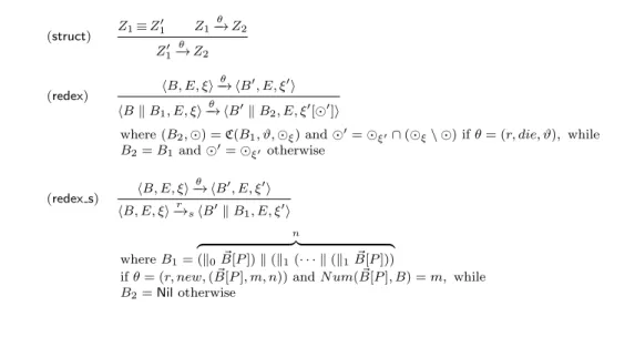
(struct) 𝑍1≡ 𝑍 ′ 1 𝑍1 𝜃 −→ 𝑍2 𝑍1′ 𝜃 −→ 𝑍2 (redex) ⟨𝐵, 𝐸, 𝜉⟩ 𝜃 −→ ⟨𝐵′, 𝐸, 𝜉′⟩ ⟨𝐵 ∥ 𝐵1, 𝐸, 𝜉⟩ 𝜃 −→ ⟨𝐵′∥ 𝐵2, 𝐸, 𝜉′[⊙′]⟩

where (𝐵2, ⊙) = ℭ(𝐵1, 𝜗, ⊙𝜉) and ⊙′= ⊙𝜉′∩ (⊙_𝜉∖ ⊙) if 𝜃 = (𝑟, 𝑑𝑖𝑒, 𝜗), while

𝐵2= 𝐵1and ⊙′= ⊙𝜉′ otherwise (redex s) ⟨𝐵, 𝐸, 𝜉⟩ 𝜃 −→ ⟨𝐵′_{, 𝐸, 𝜉}′_⟩ ⟨𝐵, 𝐸, 𝜉⟩−→𝑟 𝑠⟨𝐵′∥ 𝐵1, 𝐸, 𝜉′⟩ where 𝐵1= 𝑛 z }| { (∥0𝐵[𝑃 ]) ∥ (∥⃗ 1(⋅ ⋅ ⋅ ∥ (∥1𝐵[𝑃 ]))⃗ if 𝜃 = (𝑟, 𝑛𝑒𝑤, ( ⃗𝐵[𝑃 ], 𝑚, 𝑛)) and 𝑁 𝑢𝑚( ⃗𝐵[𝑃 ], 𝐵) = 𝑚, while 𝐵2= Nil otherwise

Table 5: BetaSIM reduction rules Now, we can introduce the last three reduction rules.

The struct rule, which is standard in reduction semantics, equates the behaviours of structurally congruent 𝛽-systems.

The redex rule is used to collect the context and uses a function ℭ : ℬ × 𝜗 × ⊙ → ℬ, deﬁned on the structure of labeled bio-processes in the following way: ℭ(𝜗′𝐵[𝑃 ], 𝜗, ⊙) =⃗ ⎧ ⎨ ⎩ (Nil, ⊙′) if ∃ Δ, Γ ∈ 𝑇 : 𝜗Δ⊙𝜗′Γ and ⊙′ _{= {(𝜗} 0Δ, 𝜗1Γ) ∈ ⊙ : 𝜗0 = 𝜗′∨ 𝜗1 = 𝜗′} (𝜗′𝐵[𝑃 ], ⊙) otherwise⃗ ℭ(𝜗′𝐵[𝑃 ] ∥ 𝐵, 𝜗, ⊙) = ℭ(𝜗⃗ ′𝐵[𝑃 ], 𝜗, ⊙) @ ℭ(𝐵, 𝜗, ⊙)⃗

(26)

where the function @ is deﬁned in the following way: (𝜗𝐵, ⊙)@(𝜗′𝐵′, ⊙′) = (𝜗𝐵 ∥ 𝜗′𝐵′, ⊙ ∪ ⊙′).

The function ℭ takes as parameters a bio-process, a label 𝜗 and a relation ⊙ and returns a bio-process, obtained from 𝐵 where all the boxes connected with the box with label 𝜗 are eliminated, and the ⊙′ relation, containing all the bindings associated to the eliminated boxes. The global effect of the application of the function ℭ in the derivation tree is to eliminate all the boxes belonging to the same complex to which the box that performs a 𝑑𝑖𝑒 action is part. The redex s rule is used for constructing the actual transition relation. We introduce this additional level of derivation because of the presence of a particular type of new event, which is enabled only if the global system satisfies a condition. Since the operational semantics is compositional, we decided to add a final reduction rule that performs the check for the global condition and that represents the transition relation of our stochastic reduction system. Formally,

Deﬁnition 12. The 𝛽-binders Stochastic Transition System ( STS) is re-ferred as 𝒮 = (𝒵, −→𝑟 𝑠, 𝑍0), where 𝒵 is the set of well-formed 𝛽-systems,

𝑍0 ∈ 𝒵 is the initial 𝛽-system and 𝑟

−

→𝑠 ⊆ 𝒵 × ℝ × 𝒵 is the stochastic

reduction relation, where 𝑟 is a stochastic rate.

The deﬁnition of STS is built upon the set of well-formed 𝛽-systems 𝒵. We now show that structural congruence and −→𝑟 𝑠 reduction preserve the

well-formedness of 𝛽-systems.

Properties 1. Let 𝒵 be the set of well-formed 𝛽-systems and 𝑍 = ⟨𝐵, 𝐸, 𝜉⟩ ∈ 𝒵. For each 𝛽-system 𝑍′ _{= ⟨𝐵}′_{, 𝐸}′_{, 𝜉⟩ such that 𝑍 ≡ 𝑍}′ _{it holds 𝑍}′ _{∈ 𝒵.}

Proof. It is straightforward to see that the rules for the structural congruence preserve the well-formedness property for bio-processes and event lists. Moreover, since the status of the all the elementary beta binders and the locations associated to boxes does not change and the environment remains unchanged, then the prop-erty reported in the Def. 9 continues to hold, and 𝑍′ preserves the well-formedness property.

Properties 2. Let 𝒵 be the set of well-formed 𝛽-systems and 𝑍 = ⟨𝐵, 𝐸, 𝜉⟩ ∈ 𝒵. For each 𝛽-system 𝑍′ _{= ⟨𝐵}′_{, 𝐸}′_{, 𝜉}′_{⟩ such that 𝑍}₋_→𝑟

𝑠𝑍′ it holds 𝑍′ ∈ 𝒵.

Proof. We report here a sketch of the proof. The property is proved by analyzing the structure of the derivation tree for −→𝑟 _𝑠 transitions. In general, each derivation

(27)

tree has the form: 𝑎𝑥𝑖𝑜𝑚 𝑍0 𝜃 − → 𝑍₀′ 𝑍1 𝜃 − → 𝑍₁′ .. . 𝑍 ≡ 𝑍𝑛 𝑍𝑛−→ 𝑍𝜃 𝑛′ 𝑍−→ 𝑍𝜃 _𝑛′ 𝑍−→𝑟 𝑠𝑍′

where all the struct reduction can be applied together after the whole context has been collected. Notice that the application of the rule struct, because of the Property 1, preserves the well-formedness property. Moreover, it is straightword to see that, in the case the function ℭ is not applied, also the redex rule preserves the well-formedness property.

For monomolecular axioms intra, hide, unhide, change, expose and tau, and bimolecular axioms inter c and inter, at the end of the derivation we have that the lists 𝐸 and 𝐸′ are structurally congruent and conditions on the rules preserve the well-formedness on the bio-process 𝐵′. Moreover, since the status of elementary beta binders and locations associated to boxes does not change and 𝜉 = 𝜉′, then the property reported in the Def. 9 continues to hold, and 𝑍′ preserves the well-formedness property. In this cases, since the label 𝜃 is empty, no modiﬁcations in the resulting 𝛽-system caused by the propagation of label informations is produced. Now consider the axioms new and delete. They cause, respectively, the creation of a number of new boxes and the elimination of a box. However, the created and eliminated boxes does not contain elementary beta binder in complexed status (because the related events are well-formed) and hence no modiﬁcations in the environment are produced. No information through labels 𝜃 is propagated along the derivation tree and the function ℭ is never called. Therefore, at the end of the derivation the lists 𝐸 and 𝐸′ are structurally congruent and the bio-process 𝐵′ is well-formed; indeed, in case of axiom new only well-formed boxes are added, while in the case of axiom delete the bio-process remains obviously well-formed. Hence 𝑍′ preserves the well-formedness property.

The execution of the axiom new c is similar to the execution of the axiom new, but an information through the label 𝜃 is propagated along the derivation three. However, because of the structure of 𝜃, also inthis case the function ℭ is never called and in the application of the ﬁnal reduction rule redex s, if the condition associated to the new event holds, only well-formed boxes without elementary beta binders in complexed status are added. Therafter, also in this case 𝑍′ preserves the well-formedness property.

(28)

in the structure of the complexation relation ⊙𝜉of the environment. In particular,

each couple (𝛾, 𝛾′) ∈ ⊙𝜉 such that 𝛾′ refers to an eliminated box, is substituted

with a new couple (𝛾, 𝛾′′) ∈ ⊙𝜉′ such that 𝛾′′ refers to a new created box, and

no elementary beta binders in complexed status without a corresponding relation in ⊙𝜉′ are created. Hence, because of the well-formedness of the events join and

split and the conditions on their axioms, no bindings are lost and no inconsistent complexed beta binders are added. Moreover, no information through labels 𝜃 is propagated along the derivation tree and also in this case the function ℭ is never called. Moreover, 𝐵′ is obtained from 𝐵 by substituing well-formed boxes with other well-formed boxes and 𝐸′ is congruent to 𝐸. Therefore, 𝑍′ preserves the well-formedness property.

Finally, consider the axiom die. In the case the box that performs the die action is not part of a complex the derivation is similar to the one already explained. Otherwise, modiﬁcations in the resulting 𝛽-system are generated also along the derivation tree and in particular, the function ℭ is called for each application of the redex reduction rule. At the end of the derivation, in the resulting 𝛽-system, all the boxes belonging to the same complex to which the box that performs the die action is part and the related bindings in the environment are eliminated. Notice that the Def. 11 guarantees that the elimination of a complex and its bindings does not corrupt the consistency of the remaining 𝛽-system, and hence the property reported in the Def. 9 continues to hold. Moreover, since 𝐵′ is obtained from 𝐵 by only eliminating boxes and 𝐸′ is obviously congruent to 𝐸, then 𝐵′ and 𝐸′ are well-formed and also in this case 𝑍′ preserves the well-formedness property.

3.4 Other language constructs

In the 𝛽-simulator (Section 7) a join event of the form:

( ⃗𝐵0[𝑃0], ⃗𝐵1[𝑃1] : 𝑟) join

is provided. This event produces a box ⃗𝐵2[𝑃2] where ⃗𝐵2 is obtained from

⃗

𝐵0 and ⃗𝐵2 as the union of the two lists, while 𝑃2 is the parallel composition

(with the proper substitutions) of 𝑃0 and 𝑃1. For example, the event:

(𝛽(𝑥, 𝑟, Δ) 𝛽(𝑦, 𝑠, Γ)[𝑃0], 𝛽(𝑧, 𝑡, Δ)[𝑃1] : 𝑟) join

produce the box:

𝐵′ = 𝛽(𝑥, 𝑟, Δ) 𝛽(𝑦, 𝑠, Γ)[𝑃0∣𝑃1{𝑥/𝑧}]

We prefer to avoid the explicit introduction of this event in the BetaSIM language because it is only syntactic sugar. Indeeed, the same result can be

(29)

obtained by deﬁning the event:

(𝛽(𝑥, 𝑟, Δ) 𝛽(𝑦, 𝑠, Γ)[𝑃0], 𝛽(𝑧, 𝑡, Δ)[𝑃1] : 𝑟) join(𝐵′)

4 System architecture

The BetaSIM stochastic simulator (hereafter 𝛽-simulator) is the core part of the system. In this section we describe the logical structure of the simulator, the algorithm and data structures it uses as well as the time evolution of a simulation.

4.1 BetaSIM ’s logical blocks

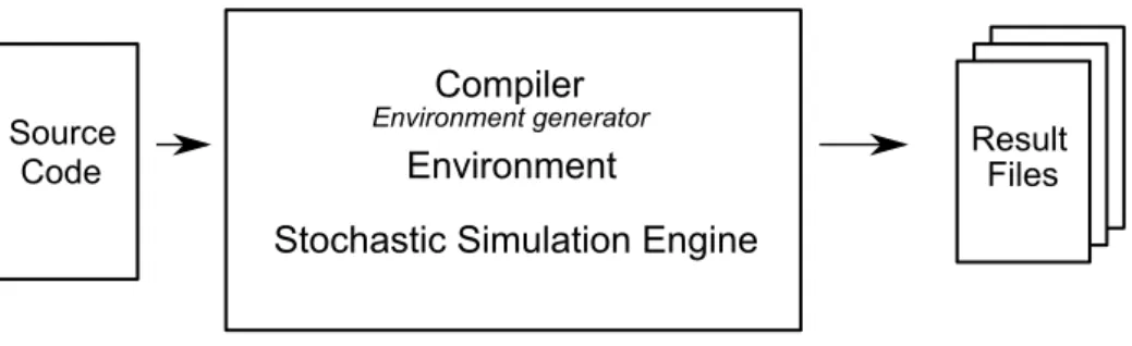
The simulator is built as a composition of three logical blocks (see Fig. 2): the compiler, the environment and the stochastic engine.

Figure 2: The logical structure of the simulator

The compiler translates the source code (a bio-process with a descrip-tion of its types and a list of events) into a runtime representadescrip-tion that is then stored into the environment. The environment provides the stochastic simulation engine with primitives for checking the state of each entity in the model, create new entities and modify them. The stochastic simulation engine drives the simulation handling the time evolution of the environment in a stochastic way and preserving the semantics of the language.

4.1.1 The compiler

The compiler parses the syntactic deﬁnition of bio-processes, complexes, events and semantic rules are codiﬁed into the data structures Entities, Complex-graphs and Elements.

(30)

4.1.2 The environment

The environment stores the data structures produced by the compiler This representation is dynamic, as opposed to the the source code which is static. At each time step, the environment holds the current state of the system:

∙ which entities (species) are present, and their cardinality; ∙ which complexes are present, and their cardinality;

∙ the active actions, e.g. actions that can be executed to make the system evolve to the next state, with their next “execution” time;

Figure 3: Main classes for environment management

Entities are the representation in the environment of equivalence classes of structural congruent processes. The algorithm to decide whether two bio-processes are congruent is polynomial in time and it is described in details in [18]. The environment assigns to each entity in the system an unique identifier ID. This ID is used to identify them in an efficient and unique way. Our concept of entity maps directly to the concept of molecular or biological species used in the definition of the Gillespie’s stochastic simulation algorithm [10].

The main classes for environment management are depicted in Fig. 35_.

An object of type element is an object with a timed event, an action that will

(31)

modify the environment at a given time by acting on entities. For example, a bimolecular element interprets a bimolecular reaction, involving exactly two source entities and two target entities:

𝐴 + 𝐵 ⇀𝐾𝐴𝐵 _𝐴′_{+ 𝐵}′

For other elements, like events, the number of aﬀected entities is variable, but always ﬁnite.

Entities are a special case of element too: it is not only the target of external (or environment) actions, but also both the source and the target of internal (or intra) actions. Delays, internal communications, binder mod-iﬁcations are all examples of actions originated by an entity that aﬀect the entity itself (and, possibly, another entity). Therefore, the timed event of an entity is the fastest intra action. Intra actions are modelled by objects of type elementMono. Their name is due to the fact that their execution interprets a monomolecular reaction:

𝐴 ⇀𝐾𝐴 _𝐴′

In the simulator architecture, bind and unbind elements are used to sim-ulate complexation actions, while complexed entities are stored in a Complex structure. Complex is a facade class to hold the internal representation of complexes as graphs of entities (Complex Graph, CG Node and CG Edge classes).

Entities, complexes and elements are held by the system in associative arrays (in Figure 3 the map for complexes Complex Rel is shown) to provide a convenient access to them and to make possible the implementation of an eﬃcient algorithm for stochastic simulation.

4.1.3 The simulation engine

The simulation engine relies on a stochastic selection algorithm. A simulation represents a trajectory in the STS generated by the initial 𝛽-system. Our simulation engine implements an eﬃcient variant of the Gillespie’s algorithms described in [8, 10].

The two level nature of the 𝛽-binders language, with its intra and inter actions, requires special care for a correct and eﬃcient implementation.

We implemented a new algorithm, called Next Action Method , that uses eﬃcient data structures that complement the structures of the environment and a new selection procedure to achieve a correct and performant stochastic simulation.

The data structures used by the Next Action method are three: the Env List, the Env Map and the Action Queue (see Fig. 4).

(32)

Env List Element x … i, j Element z … j, k Element y … i 2 1 i k j … … T1 T2 T3

Env Map Action Queue

Figure 4: The data structures used by the Next Action Method

The Env list holds the list of all the elements (i.e. of all the possible actions) of the system. The stochastic selection algorithm chooses the fastest action from this list and makes the system evolve accordingly.

The Env map is an associative array that holds the dependency relations between entities and elements in the system. Consider as an example a bio-processes 𝐵1, involved in two reactions:

∙ it can perform an inter-communication, represented by a Bimolecular element 𝑏𝑖𝑚 in the environment, so that 𝑏𝑖𝑚 ::= 𝐵1 + 𝐵2 ⇀ 𝐵1′ + 𝐵

′ 2;

∙ it can perform an intra-communication, represented by the Entity ele-ment 𝐵1 itself, so that 𝐵1 ⇀ 𝐵3.

The Env map entry for the 𝐵1 entity will be 𝐸𝑛𝑣𝑀 𝑎𝑝[𝐵1] = {𝐵1, 𝑏𝑖𝑚}.

Intuitively, for every entity there is an entry in the Env map that holds a list of the elements whose timing can be aﬀected by the entity considered.

The action queue is an indexed priority queue implemented as an heap [19]. The queue holds elements ordered by their next reaction time. This semi-ordered data structure allows us to implement the min operation in constant time, overcoming the principal limitation of the environment list. Updat-ing the position of an element in the queue, an operation that must be performed when the next execution time for that element is re-computed, requires 𝑂(log 𝑛) time.

The Beta Workbench

Technical Report CoSBi 03/2007

The Beta Workbench

The Beta Workbench

Alessandro Romanel, Lorenzo Dematt´

e and Corrado Priami

The Microsoft Research - University of Trento

Centre for Computational and Systems Biology

Contents

1

Introduction

2

Related work

3

The Language

3.1

The syntax

∣

∣

∣

∣

∣

∣

∣

∣

∣

∣

∣

∣

∣

∣

∣

∣

∣

∣

∣

∣

∣

∣

∣

3.2

The operational semantics

∣

∣

∣

∣

3.3

The stochastic transition system

3.4

Other language constructs

4

System architecture

4.1

BetaSIM ’s logical blocks