UNIVERSITY
OF TRENTO
DEPARTMENT OF INFORMATION AND COMMUNICATION TECHNOLOGY
38050 Povo – Trento (Italy), Via Sommarive 14 http://www.dit.unitn.it
THEORETICAL INTERPRETATIONS AND APPLICATIONS
OF RADIAL BASIS FUNCTION NETWORKS
Enrico Blanzieri
May 2003
Theoretical Interpretations and Applications
of Radial Basis Function Networks
Enrico Blanzieri
11Department of Information and Communication Technology University of Trento
via Sommarive 14 I-38050 Povo - Trento Italy Phone: +39 0461 882097
Fax: +39 0461 882093 Mobile phone: +39 3402588468
Abstract
Medical applications usually used Radial Basis Function Networks just as Artifi-cial Neural Networks. However, RBFNs are Knowledge-Based Networks that can be interpreted in several way: Artificial Neural Networks, Regularization Networks, Support Vector Machines, Wavelet Networks, Fuzzy Controllers, Kernel Estimators, Instanced-Based Learners. A survey of their interpretations and of their correspond-ing learncorrespond-ing algorithms is provided as well as a brief survey on dynamic learncorrespond-ing algorithms. RBFNs’ interpretations can suggest applications that are particularly interesting in medical domains.
Key words: Radial Basis Function Networks, Support Vector Machines, Regularizations, Wavelet Networks, Kernel Estimators.
1 Introduction
Since their first proposal Radial Basis Function Networks [58] (in the following simply referred to as RBFNs) has been widely used in applications. Theoretical results showing their interpretability in terms of other systems and methods accumulated. In particular, they interpretability in terms of fuzzy logic and probabilistic rules was noted [44,11,79,80] putting RBFNs in the wider family of Knowledge-Based Neurocomputing [22]. However, in medical applications RBFNs seems to be used simply as suitable alternatives to more popular Artificial Neural Networks (ANNs) as the Multilayer Perceptron (MLP) (see [11] for an exception). The goal of this paper is to survey several theoretical interpretations of RBFNs emphasizing the properties they entail and their potential application consequences in medical domains.
The architecture underlying RBFNs has been defined and presented several times under different names. Initially presented in the neural network frame-work [58] RBFNs were reintroduced as a particular case of regularization net-works [68]. Support Vector Machines [23] reintroduced RBFNs again in the framework of Statistical Learning Theory and Kernel-Based Algorithms [59]. The architecture of Wavelet Networks [91] is a particular case of RBFNs. In-dependently, the fuzzy logic community developed fuzzy controllers [6] whose effectiveness rely on the same approximation principles [44]. Closely related to the fuzzy approach some research [11,79,80] proposed to use the RBFN for mapping and refining propositional knowledge. With a very different ap-proach in the mainstream of applied statistics [75], the problem of regression and classification, and more generally density estimation, were faced by means of kernel estimators that were strongly related to RBFN. Finally, RBFN can also be placed in the framework of instance based learning [57]. As a conse-quence RBFNs can be viewed from several different points of view.
Medical applications usually used RBFNs as an ANN. RBFNs were exploited in medical domains such as surgical decision support on traumatic brain injury patients [53], coronary artery disease from electrocardiography (ECG) [25,52], classification of cardiac arrhnythmias from ECG [1], diagnostic ECG classi-fication [14], prevision of heart rate [39] and analysis of its variability [7,63], ischemia detection [8], spectroscopic detection of cervical precancer [81], es-timation of evoked potentials [34] and of neural activity [2] and prognosis of intensive care-unit patients [11].
Different interpretations of RBFNs lead to rather different learning algorithms. The distinction between static and dynamic learning algorithms for RBFNs is relevant. The static learning algorithms modify the parameters of the RBFN given a fixed number of basis functions. The dynamic learning algorithms mod-ify the number of basis functions of the network, integrating the actions
occur-ring in the initialization and in the refining phases in an incremental learning algorithm. An excellent survey of static learning algorithms for RBFNs has been recently proposed [74].
The goal of this paper is to survey the different interpretations of RBFNs in order to emphasize relevant properties of RBFNs that can be useful for a reader interested in medical applications. A complete and exaustive survey on RBFNs applications in the area of biomedicine goes beyond the scope of this paper. Moreover, it’s not our goal to provide a unique formal framework for different types of systems as done in [70]. Our aim is rather to focus the atten-tion to properties of the RBFNs that can be useful for medical applicaatten-tions. Some of these properties depend upon the fact the RBFNs can be interpreted in rather different ways. As an example, we consider the scenario of melanoma early diagnosis support addressed by MEDS [10,73] where the combination of different classifiers was exploited in order to reach the required performance. The task is to support the diagnosis of melanoma from digital images of pig-mented skin lesion acquired by means of digital epi-luminescence microscopy (D-ELM). In such a scenario, sensitivity and specificity are the main issues but, given the so called ABCD rule (Area, Border, Color, Dimension) used by the dermatologists, comprehension of the elaboration is important. The task also requires feature extraction from images and possibly the use of clin-ical information. Moreover, the scarce quantity of data available hardens the learning task.
The paper is composed of two complementary parts. The first part (Sections 2 and 3) surveys the scientific literature related to RBFNs. The second part (from Section 5 to Section 12) addresses the connections between RBFNs and other methods and approaches. Concluding remarks are presented for each single section of the second part. More in detail, Section 2 describe the basic RBFN architecture and their approximation properties, i.e. the characteri-zation of the problems that the RBFNs can solve. Section 3 deals with the basic learning algorithms introducing the distinction between static and dy-namic learning algorithms. Section 4 considers RBFNs as Neural Networks and briefly reports on the recurrent version of the RBFNs. Section 5 6, 7 consider RBFNs as Regularization Networks, Support Vector Machines and Wavelets Networks respectively. Section 8 and 9 deals with RBFNs as fuzzy systems and their consequent symbolic interpretation. A statistical approach to RBFNs is described in Section 10. RBFNs as a type of Instance Based Learning is presented in Section 11. Section 12 briefly describes the learning algorithms with structural changes. Finally, Section 13 and Section 14 draws conclusions.
2 Architecture and Approximation Properties
The RBFNs correspond to a particular class of function approximators which can be trained, using a set of samples. RBFNs have been receiving a growing amount of attention since their initial proposal [18,58], and now a great deal of theoretical and empirical results are available.
2.1 Radial Basis Function Networks Architecture
The approximation strategy used in RBFNs consists of approximating an un-known function with a linear combination of non–linear functions, called basis functions. The basis functions are radial functions, i.e. they have radial sym-metry with respect to a centre. Let X be a vectorial space, representing the domain of the function f (¯x) to approximate, and ¯x a point in X. The general form for an RBFN N is given by the following expression:
N (¯x) =
n
X
i=1
wie(k ¯x − ¯ci ki) (1)
where e(z) is a non-linear radial function with centre in ¯ci and k ¯x − ¯ci ki
denotes the distance of ¯x from the centre and wi are real numbers (weights).
Each basis function is radial because its dependence on ¯x is only through the term k ¯x − ¯ci ki.
Many alternative choices are possible for the function e(z): triangular, car-box, gaussian. Anyhow it is usual to choose e(z) in such a way that the following conditions hold:
e(−z) = e(z)
lim
z−>±∞e(z) = 0
A common choice for the distance function k . ki is a biquadratic form:
k ¯x ki = ¯xQix¯T
Qi = qi,11 0 . . . 0 0 qi,22 . . . 0 . . . . 0 0 . . . qi,nn
In the simplest case all diagonal elements of Qi are equal qi,jj = qi so that
Qi = qiI. In this case the radiality of the basis functions is proper and if
function e(z) fades to infinity, 1
qi can be interpreted as the width of the i-th
basis function.
From the point of view of the notation is also common to write: e(k ¯x − ¯ci ki) = ei(k ¯x − ¯ci k)
where the information about the distance function k . ki is contained in the function ei(¯x).
It is also possible to define a normalized version of the RBFN: N (¯x) = Pn i=1wie(k ¯x − ¯ci ki) Pn i=1e(k ¯x − ¯ci ki) (2)
Different type of output, continuous or boolean, may be needed depending on the type of the target function. In order to obtain a boolean output NB we
need to compose function N and a derivable threshold function σ:
NB(¯x) = σ(N (¯x))
usually σ(x) is the sigmoid (logistic function):
σ(x) = 1 1 + e−kx
whose derivative is:
dσ(x)
dx = σ(x)(1 − σ(x))
The positive constant k expresses the steepness of the threshold. Alternatively, we can obtain a boolean output composing N with the function sign(x + b) where b ∈ R is a threshold.
2.2 Universal Approximators
A relevant property usually required for a class of approximators is univer-sal approximation. Given a family of function approximators, it is important to characterize the class of functions which can be effectively approximated. In general, an approximator is said to be universal if it can asymptotically approximate any integrable function to a desired degree of precision.
Hornik et al. [43] proved that any network with at least three layers (input, hidden and output layers) is an universal approximator provided that the acti-vation function of the hidden layer is nonlinear. In the Multi-Layer Perceptron (MLP), traditionally trained by means of the backpropagation algorithm, the most frequently used activation function is the sigmoid. RBFNs are similar to MLPs from the point of view of the topological structure but they adopt activation functions having axial symmetry.
Universal approximation capability for RBFNs was presented in [65,64], where the problem of characterizing the kinds of radial function that entail the prop-erty of universal approximation was addressed by Chen and Chen [21] who shown that for a continuous function e(z) the necessary and sufficient condi-tion is that it is not an even polynomial.
From the mathematical point of view the universal approximation property is usually asserted by demonstrating the density of the family of approxi-mators into the set of the target functions. This guarantees the existence of an approximator that with a high, but finite number of units, can achieve an approximation with every degree of precision. The result states only that this approximator exists. It does not, however, suggest any direct method for constructing it. In general this assertion is true, even when the function is explicitly given. In other words, it is not always possible to find the best approximation within a specified class of approximators, even when the ana-lytical expression of the function is given.
2.3 The Function Approximation Problem
Whether the target function is boolean or continuous, the learning task of a feed–forward RBFN can be stated as a classification or regression problem. In both cases the problem can be stated in the general framework of the function approximation problem, formally expressed as: given an unknown target function f : Rn→ D and a set S of samples (x
i, yi) such that f (xi) = yi
for i = 1 . . . N . find an approximator ˆf of f that minimizes a cost function E(f, ˆf ). Function f is a mapping from a continuous multidimensional domain X to a codomain D ⊂ R (regression) or D = B = {0, 1} (classification).
The approximation accuracy is measured by the cost function E(f, ˆf ) also said error function (or approximation criterion) and which depends on the set of examples S. In general the solution depends upon S, upon the choice of the approximation criterion and upon the class of functions in which we approximator ˆf is searched. In practice, a common choice for the cost function is the empirical square error:
SEemp= N X i=0 (yi− ˆf (xi)) 2 (3)
Under some restrictive hypothesis it can be shown that minimizing (3) is equivalent to finding the approximator that maximizes the likelihood of S, i.e. the probability of observing S given the a priori hypothesis f = ˆf (P (S/f = ˆf ) [57].
Given a family of approximators the optimal one minimizes the error in (3). Finding the optimal approximator is thus equivalent to solving a least squared error problem.
It is worth noting, that the problem definition and the considerations about the errors, can be extended to the case in which a subset of the dimension of the domain is boolean and so the domain is the Cartesian product of a n-dimensional continuous space to a m-dimensional boolean space Rn× Bm.
The boolean inputs can be viewed as continuous inputs that receive only the boolean values 0 and 1.
3 Learning Algorithms for RBFNs
The universal approximation property states that an optimal solution to the approximation problem exists: finding the corresponding minimum of the cost function is the goal of the learning algorithms. This section introduces some of the basic facts about learning algorithms for RBFNs. More advanced learning methods are presented in the Sections 5-12.
In the following we will assume that the choice of the radial basis function e(z) has already been made. In order to find the minimum of the cost function a learning algorithms must accomplish the following steps:
(1) select a search space (i.e. a subset of the parameter space); (2) select a starting point in the space (initialization);
An RBFN is completely specified by choosing the following parameters: • The number n of radial basis functions;
• The centres ci and the distances k . ki, i.e. the matrices Qi (i = 1 . . . n);
• The weights wi.
The number n of radial functions is a critical choice and depending on the approach can be made a priori or determined incrementally. In fact, both the dimensions of the parameter space and, consequently, the size of the family of approximators depend on the value of n. We will call an algorithm that starts with a fixed number n of radial functions determined a priori ’static,’ and an algorithm that during the computation is able to add or delete one or more basis functions ’dynamic.’ A static learning algorithm is also parametric because the search for the optimal approximator corresponds to a search in the parameter space defined by the fixed number of radial basis functions. On the contrary, a dynamic learning algorithms changes the parameter space in which it operates, while adding or deleting radial basis functions. The learning algorithms are also very different depending on whether the sample set S is completely available before the learning process or if it is given, sample by sample, during training. In the former case, off–line learning is possible while in the latter, an on-line learning approach is needed. While some of the static algorithms can be adapted for both learning types, the application of the dynamic one makes sense only in the case of on-line learning.
The static methods for learning RBFNs from examples are based on a two– step learning procedure: first the centres and the widths of the basis functions are determined and then in a second step the weights are determined. Each one of the steps can be done by means of several different strategies. A usual training procedure uses a statistical clustering algorithm, such as k-Means for determining the centres and the widths associated to the basis functions and then estimates the weights by computing the coefficients of the pseudo-inverse matrix or, alternatively, by performing the error gradient descent.
Given n, the corresponding parameter space is defined by the parameters that characterize each one of the radial basis functions, i.e. the centres ci and the
matrices Qi, and the weights wi (i = 1 . . . n).
The search space can be restricted, by limiting the possible choices of the parameters, or imposing constraints on the values. Several basic techniques are available for initializing and refining an RBFN. Some of them apply to all kinds of parameter in the network, some not.
3.0.0.1 Gradient Descent. Using continuous radial functions derivable in the whole parameter space, it is immediatly possible to apply the classical
error gradient descent technique, in order to finely tune not only the weights wi but also the centres ci and the elements of the matrix Qi in the first hidden
layer units. More specifically, let SEemp be the quadratic error evaluated on
the learning set and let λk indicate a generic parameter in the network, such
as a weight wi on a link, or an element of the matrix of the width Qi or a
component of the centre ¯ci of a radial function, all the necessary derivatives
can be easily computed, and the learning rule takes the form: ∆λk = −η
∂SEemp
∂λk
(4) where η is the learning rate. The main problems with gradient descent are that the convergence is slow and depends on the choice of the initial point. Although Bianchini et al. [9] demonstrated that, in the case of classification, a wide class of RBFNs has a unique minimum, (i.e. no local minima exists in the cost function) it is not possible to reach this optimal point, in a short time, from every starting point of the parameter space. Hence the initialization of the network is critical. Giordana and Piola [35] showed that the adaptation of all the parameters (namely, centres, widths, and weights) can lead to a misbehavior of the gradient descent procedure for some value of the learning rate and proposed a remedy. Optimized versions of the gradient descent tech-nique such as conjugate gradient, momentum or others are possible. It is also possible to use the so-called on-line gradient descent. Analysis of the learning behavior of on-line gradient descent has been proposed by Freeman and Saad [30] and more recently by Marinaro and Scarpetta [54] who showed that for RBFN with radial Gaussian and n > |X|, namely number of centres greater than the number of inputs, no plateau of the generalization error is produced.
3.0.0.2 Instance-Based Initialization. In the first formulation of RBFNs [58] all instances of the sample set S were used as centres of the basis func-tions and the width of the basis function were the same for all the funcfunc-tions of the network. This technique is very simple but produces excessively large networks which are inefficient and sensitive to overfitting, and exhibit poor performance.
3.0.0.3 Centre Clustering. A partial solution to the problems of Instance-Based initialization is to cluster similar samples together, adopting a well– known technique (clustering), widely used in Pattern Recognition. The tech-nique assigns a corresponding centroid to every cluster, i.e. a real or artificial sample that appears to be prototypical for the cluster. The centroid is then chosen as the centre for a radial basis function. The resulting network is re-markably smaller than when Instance Based Learning is used. Moreover in this case the centres can also be tuned via gradient descent. This basic technique
also permits the radial condition to be relaxed, adopting different widths along different dimensions of the domain X. The parameter space contains all the centre values and the width values so it is larger than in the other case. The price to pay for better performance is an increase in the training time. Several clustering techniques are useful for the task, like k-means or fuzzy clustering [66]. An interesting version is input/output clustering where the input and output vectors are concatenated before the clustering process. The technique was already used in practice (for example in [11]) and a deeper analysis of it has been proposed recently [83].
3.0.0.4 Symbolic Initialization. An alternative method for constructing the layout, i.e. choosing the centres and the corresponding widths of an RBFN is to use a symbolic learning algorithm [4,79]. This becomes particularly simple in the case of Factorizable RBFNs (F-RBFNs). In this case the factorization permits seeing each factor of the radial function as a fuzzy membership of widths Aij determined by the width of the basis function and the product as a
logical AND, so that F-RBFN can be approximated by a set of propositional clauses of the type:
Rj = member(x1, A1j) ∧ member(x2, A2j) ∧ . . . (5)
. . . ∧ member(xn, Anj) → wj
Rules of this type can be easily learned using an algorithm for inducing decision trees, such as ID3 [69,72] or, better an algorithm for inducing regression trees, such as CART [17]. Initialization of RBFNs by means of decision trees has been proposed by [5] and extensively analysed by Kubat [51].
3.0.0.5 Weights Linear Optimization. Both equations (1) and (2) are linear in the weights wi hence, given the parameters ci and Qi of the basis
functions it is possible to use a linear optimization method for finding the values of the wi, that minimize the cost function computed on the sample set.
This is the learning strategy adopted in the regularization theory approach [68]. This method relies on the computation of the pseudo-inverse matrix. This point will be addressed in detail in Section 5 where the links between RBFNs and regularization theory are discussed. Further optimizations of the method have been presented [20] [61]. In particular Chen et al. [20] exploited orthogonal decomposition in their Orhogonal Least Squares algorithm (OLS). Recently recursive versions of OLS has been proposed and applied also to the selection of the centres [37].
3.0.0.6 Basis Function Learning, Above we have made the assumption that the choice of the radial function e(z) has already been made. However, Webb and Shannon [85] explored the possibility of learning the shape of the basis function. Their work shows that the adaptive shape RBFNs generally achieve lower error than the fixed shape networks with the same number of centres.
3.0.0.7 Evolutionary Computation. Evolutionary computation can be applied to the learning algorithms of RBFNs [86,27]. In general evolutionary computation is a powerful search strategy that is particularly well suited to application in combinatory domains, where the cross–over of locally good solu-tions can lead to better global solusolu-tions. That seems to be the case for RBFNs. In fact the RBFNs architecture is based on a local strategy of approximation: the different functions interact poorly with each other and so allow their com-binations to be significantly better than the original networks. As long as the intermediate solutions have a variable number of basis functions the methods could be classified as dynamic, static otherwise.
4 RBFNs as Neural Networks
RBFNs can be described as three layer neural networks where hidden units have a radial activation function. Although some of the results of the neu-ral networks can be extended to RBFN, exploiting this interpretation (e.g. approximation capabilities [43] and the existence of a unique minimum [9], substantial differences still remain with respect to the other feed–forward net-works. In fact, RBFNs exhibit properties substantially different with respect to both learning properties and semantic interpretation. In order to under-stand the different behaviours of the two network types, assume we have to modify a weight between two nodes in the Multi Layer Perceptron (MLP), as is done by the backpropagation updating rule during the training phase. The effect involves an infinite region of the input space and can affect a large part of the co-domain of the target function. On the contrary, changing the amplitude of the region of the input space in which the activation function of a neuron in an RBFN fires, or shifting its position, will have an effect local to the region dominated by that neuron. More in general, this locality property of RBFNs allows the network layout to be incrementally constructed (see for instance [55]), adjusting the existing neurons, and/or adding new ones. As every change has a local effect, the knowledge encoded in the other parts of the network is not lost; so, it will not be necessary to go through a global revision process.
hidden units, we see that each neuron, apart from a narrow region where the sigmoid transient occurs, splits the input domain into two semi-spaces where its output is significantly close to 1 or to 0. The whole semispace where the output is close to 1 contributes to the value of the target function. On the contrary, in an RBFN, each hidden neuron is associated to a convex closed region in the input domain (activation area), where its response is significantly greater than zero, and dominates over every other neuron. The greatest con-tribution of a neuron to the output value Y comes essentially from this region. On the contrary, RBFNs, while similar in the topological structure, make use of activation functions having axial symmetry. As a consequence, MLP and RBFNs encode the target function in a totally different way.
Most attention in the ANN literature is focused on feed–forward networks, but there is a growing interest in networks provided with feedback called Re-current Networks [26]. A reRe-current network is characterized by having some output units connected with some units of the other layers. This apparently simple modification causes heavy changes in behaviour and computational properties of a network. Owing to the presence of feedback arcs, a network becomes an approximator of dynamical systems. Frasconi et al. [29] intro-duced a second order RBFNs where the feedback connections are obtained via a product. It is shown how these networks can be forced to work as finite state automata. The authors report examples where a recurrent RBFN learns a Tomita grammar and provide an algorithm for extracting symbolic descrip-tion of the corresponding automaton. Not directly interpretable as RBFN the networks proposed in the work of Kim and Kasabov [49] shows the power that a recurrent architecture can provide and their approach proved to be effec-tive in a biologic context [60]. Further investigation is still required to test possible relations with other formalisms like Feature Grammars and Markov Chains that could emerge from a recurrent generalization of the symbolic and statistical interpretations (see Sections 9 and 10).
4.0.0.8 Concluding Remarks. In this framework, the basic learning tech-nique is gradient descent. Using an F-RBFN with factors that appear in more than one product Back-Propagation training can be used as is usually done for MLPs. As was noted in Section 3, the initialization is critical and is usually achieved using the whole data set or a clustering technique. The convergence of gradient descent algorithms is guaranteed only in the case of off-line learning. Empirically, an on-line version appear to converge reasonably well. Dynamic versions were presented by Platt [67] and, combined with an on-line clustering algorithm by Fritske [32]. As noted in the introduction, most of the medi-cal applications considers RBFNs as ANNs. The melanoma diagnosis scenario provides a natural application for ANNs (see references in [10]).
5 RBFNs as Regularization Networks
In a paper that is fundamental for RBFN theory Poggio and Girosi [68] pro-vided an elegant connection with Kolmogorov regularization theory. The basic idea of regularization consists of reducing an approximation problem to the minimization of a functional. The functional contains prior information about the nature of the unknown function, like constraints on its smoothness. The structure of the approximator is not initially given, so in the regularization framework the function approximation problem is stated as:
Find the function F (x) that minimizes:
E(F ) = 1 2 n X i=1 (di− F (xi))2+ λk P F k2 = Es(F ) + λEc(F ) (6)
Where ES(F ) is the standard error term, ER(F ) is the regularization term, λ
is a regularization parameter and P is a differential operator. By differentiating equation (6) we obtain
P∗ P F (x) = 1 λ n X i=1 (di− F (xi))δ(x − xi) (7)
where δ(.) is Dirac’s function. The solution F of equation (7) is finally:
F (x) = 1 λ n X i=1 (di− F (xi))G(x, xi) (8)
Regularization theory leads to an approximator that is an expansion on a set of Green’s functions G(x, xi) of the operator P∗P . By definition Green’s
function of the operator A centred in xi is
AG(x, xi) = δ(x − xi)
The shape of these functions depends only on the differential operator P , i.e. on the former assumptions about the characteristics of the mapping between input and output space. Thus the choice of P completely determines the basis functions of the approximator. In particular if P is invariant for rotation and translation Green’s function is:
so they depend only on the distance k x − xi k and are therefore Radial
Functions.
The points xi are the centres of the expansion and the terms 1λ(di− F (xi)) of
equation (8) are the coefficients. The approximator is
wi = λ1(di− F (xi)) F (x) =Pni=1wiG(x, xi) (9)
Equation (9) evaluated in the point xj leads to
F (xj) = n
X
i=1
wiG(xj, xi) (10)
In order to determine the wi let us define the matrices:
F = F (x1) F (x2) ... F (xN) d = d1 d2 ... dN W = wi w2 ... wN G = G(x1, x1) G(x1, x2) ... G(x1, xN) G(x2, x1) G(x2, x2) ... G(x2, xN) ... ... ... ... G(xN, x1) G(xN, x2) ... G(xN, xN)
Then equations (9) can be represented in the form of matrices:
W = 1
λ(d − F ) F = GW Eliminating F from both expressions, we obtain:
The matrix G is symmetric and for some operator is positive definite. It is always possible to choose a proper value of λ such that G + λI is invertible, that leads to:
W = (G + λI)−1d
It is not necessary to expand the approximator over the whole data set, in fact the point xi on which equations (9) was evaluated is arbitrarily chosen. If we
consider a more general case in which the centres of the basis functions ci with
i = 1 . . . n are distinct from the data the matrix G is rectangular. Defining two new matrices as:
G0 = (G(ci, cj)) i, j = 1 . . . n
G = (G(xi, cj)) i = 1 . . . N j = 1 . . . n
the optimal weights are:
w = (GTG + λG0) −1
GTd and if λ = 0
w = (GTG)−1GTd = G+d where G+ = (GTG)−1GTd is the pseudoinverse matrix.
In the regularization framework the choice of the differential operator P de-termines the shape of the basis function. Haykin [40] reports a formal descrip-tion of the operator that leads to the Gaussian RBFN. The operator expresses conditions on the absolute value of the derivatives of the approximator. Hence the minimization of the regularization term ER(F ) causes a smoothing of the
function encoded by the approximator.
In an analogous way Girosi et al. [36] presented an extension of the regulariza-tion networks. The regularizaregulariza-tion funcregulariza-tional is mathematically expressed as a condition on the Fourier transform of the approximator. In their work they set the constraint that the bandwidth be small. Such an approximator, they ar-gue, oscillates less so it presents a smoother behaviour. They obtain the class of the generalized regularization networks strongly connected to what they called Hyper Basis Functions (HBF) that approximates the function with:
f (x) =
n
X
i=1
ci(k x − xi kW) (11)
where the weighted norm is defined as: k x kW = xWTW x, with W the vector
of weights.
The RBFN described by equation (11) is not radial. The surface with the same value of the function are not spheric any more but hyper–ellipsoidal. That is the case of the network described by equation (1).
Finally, Orr [61] exploited the regularization framework for determining a criterion for the selecting the position of the centres. As a conclusion, regu-larization theory provides a strong mathematical framework which allows an optimal estimate of the weights and, at the same time, allows smoothing of the function encoded in the RBFN, to be controlled via the regularization term.
5.0.0.9 Concluding Remarks. By applying regularization theory to RBFNs we obtain an off-line learning method: The centres of the radial basis functions are initialized with the samples or with a clustering technique, the widths are usually a fixed parameter and the weights are computed via pseudoinversion. The number of basis functions is fixed, so the method is static. The main fea-ture of the framework is to provide guidelines for an optimal choice of the type of basis functions, depending on the regularization term used for expressing the differential smoothing properties of the approximators. In other terms the choice of the radial function implicitly corresponds to a choice of a regular-ization term. Learning of the basis function has been explored in [85]. Quite often in practical applications λ = 0 and the effect of the regularization term is lost. Considering values of λ 6= 0 can be useful. An analytical justification of the shape of the radial function can improve confidence in the system. In the melanoma diagnosis scenario regularization can be explored in order to enhance the performance. However, cost-sensitiveness has to be considered.
6 RBFNs as Support Vector Machines
RBFNs are deeply related to Support Vector Machines (SVM) [23] that are learners based on Statistical Learning Theory [84]. In the case of classification the decision surface of a SVM is given in general by
SVM(¯x) = sign( ¯wφ(¯x) + b)
¯
w ∈ F and b ∈ R are such that they minimize an upper bound on the ex-pected risk. We omit the formula of the bound that represents a fundamental contribute given by Vapnik to statistical learning theory. For the present pur-pose it suffices to remember that the bound is compur-posed by an empirical risk term and a complexity term that depends on the VC dimension of the linear separator. Controlling or minimizing both the terms permits control over the generalization error in a theoretically well-founded way.
The learning procedure of a SVM can be sketched as follows. The minimization of the complexity term can be achieved by minimizing the quantity 1
2|| ¯w|| 2,
namely the square of the norm of the vector ¯w. In addition the strategy is to control the empirical risk term by constraining:
yi( ¯wφ(¯xi) + b) ≥ 1 − µi
with µi ≥ 0 and i = 1 . . . N for each sample of the training set. The presence
of the variables µi allows some misclassification on the training set.
Introducing a set of Lagrange multipliers αi i = 1 . . . N if is possible to solve
the programming problem defined above, finding ¯w, the multipliers and the threshold term b. The vector ¯w has the form:
¯ w = N X i=1 αiyiφ(¯xi)
so the decision surface is:
SVM(¯x) = sign(
N
X
i=1
αiyiφ(¯xi)φ(¯x) + b)
where the mapping φ compares only in the dot product φ(¯xi)φ(¯x). The
depen-dency only on the dot product and not on the mapping φ is valid also for the multipliers. Following [59], the connection between RBFNs and SVMs is based upon the remark that a kernel function k(¯x, ¯y) defined on k : C × C → R with C a compact set of Rn, namely
∀f ∈ L2(C) : Z
Ck(¯x, ¯y)f (¯x)f (¯y)d¯xd¯y ≥ 0
can be seen as the dot product k(¯x, ¯y) = φ(¯x)φ(¯y) of a mapping φ : Rn→ F in
some feature space F. As a consequence, it is possible to substitute k(¯x, ¯y) = φ(¯x)φ(¯y) obtaining the decision surface expressed as:
SVM(¯x) = sign(
N
X
i=1
αiyik(¯xi, ¯x) + b) (12)
Choosing a radial kernel k(¯x, ¯y) = e(||¯x − ¯y||) equation 12 has the same struc-ture of the RBFN presented in section 2.1 in the case of a classification task.
6.0.0.10 Concluding Remarks. The possibility of interpreting RBFNs as an SVM permits application of this technique to control complexity and prevent overfitting. Complexity regularization has also been studied directly for RBFNs [50] with bounds on the expected risk in terms of the sample set size. SVMs are popular. They also connect RBFNs with Kernel-Based Algorithms and, following Muller et al. [59] with Boosting techniques (see [24] for an application of Boosting to RBFNs). In the melanoma diagnosis scenario, [71] reports satisfying performance of a gaussian SVM with respect to other machine learning techniques in the task of diagnosis of pigmented skin lesions. Theoretical bounds on the generalization error can improve confidence in the system and its chances of acceptance.
7 RBFNs as Wavelet Networks
Wavelet Networks (WN) were proposed as nonparametric regressors [92,91]. The proposal relies on the results of the broad area of wavelet theory and wavelet analysis that is very popular for signal analysis and data compression. In a nutshell, the basic idea of the wavelet transform is to analyse signals in terms of local variability with more flexibility than the usual Fourier analysis. The wavelet network estimator is given by:
WN(¯x) =
K
X
i=1
βiφi(¯x)
where φi(x) is a function belonging to the set
F = {φp,v¯ = ψ− 1
2nvφ(ψ−vx − ¯¯ pτ ) : v ∈ Z, ¯p ∈ Zn}
where ψ and τ are dilation and translation step sizes and φ(x) is a radial wavelet function so it can be written as φ(x) = ξ(¯x¯xT).
WN(¯x) =
K
X
i=1
βiψ−1/2nviφ(ψ−vix − ¯¯ piτ )
with ¯pi, vi corresponding to the values of ¯p and v characterizing φi.
Eq. 7 corresponds to the RBFN of Eq. 1 where wi = βiψ−1/2nvi, ¯ci = ¯piτ ψvi,
e(||¯x − ¯ci||i) = ξ(ψvix¯¯xT) and consequently Qi = ψviI.
Informally, the RBFN corresponding to WN has centres that are distributed in the input space in a variable but regular pattern depending on the value of τ . The width of the functions depends on ψ. The learning methods are essentially based on the selection of the wavelets. The major drawback is presented by the high number of centers requested. Recently a bayesian approach was proposed in [42].
7.0.0.11 Concluding Remarks. Not all radial functions are permissible as radial wavelets so there is no general equivalence. The consequence of the connection between these methods has not been completely investigated, both theoretically and empirically. Wavelets are commonly used in signal processing (e.g. ECG or EEG). A suggestion could be that wavelets decomposition could be a viable way to insert knowledge in a RBFN network expressed in an analytical form. In the melanoma diagnosis scenario wavelets could be used to elaborate the images and RBFNs can provide a common framework for signal related features and clinical features.
8 RBFNs as Fuzzy Controllers
RBFNs can also be interpreted as fuzzy controllers [44]. In general, a controller of this kind is a software or hardware implementation of a control function, defined from the state–space of the system to its input–space. In this way, the control function maps a set of information about the state of the system we want to control, to the actions the controller has to apply to the system. Typically, the state and the actions are continuous vectors and the controller is fully described by a set of input variables X, a set of output variables Y , and the set of elements implementing the control function. In the case of fuzzy controllers, the internal elements are defined by means of a fuzzy logic propositional theory.
8.1 Fuzzy Logics
Fuzzy logics are based on a generalization of the characteristic function of a set. Formally, let fA be the characteristic function of a set A:
fA(x) = 1 if x ∈ A 0 if x 6∈ A
Fuzzy set theory [90] generalizes the notion of presence of an element in a set and consequently the notion of characteristic function, by introducing fuzzy values. This approach is equivalent to introducing uncertainty in the presence of an element in a set. In this context the fuzzy characteristic function, that is called membership, can assume any value in the interval [0, 1]. A set in which the membership function is restricted to assume the values in the set {0, 1}, is said to be crisp. The introduction of a fuzzy membership has deep implications concerning the logics which can be built on it. The first one is the possibility of having fuzzy truth values for predicates. A predicate is no longer simply false (0) or true (1) but can assume any value between. Consequently, the definitions of the basic connectives (disjunction, conjunction and negation) have to deal with fuzzy values. Fuzzy logics is typically used for expressing uncertain or approximate knowledge in the form of rules. The theory can be partially contradictory, causing fuzzy memberships to overlap each other. Many different shapes for the membership functions have been proposed (triangular, trapezoidal, gaussian) (see [6]).
8.2 Fuzzy Controllers and RBFNs
Usually a fuzzy controller is organized as three layers. The first one imple-ments the so–called fuzzyfication operation and maps every dimension of the input space via the memberships, to one or more linguistic variables, in a fuzzy logic language. The linguistic variables are then combined with the fuzzy con-nectives to form the fuzzy theory. Typically the theory is propositional and it can be flat or not, e.g. expressed as a sum of minterms. Finally, the last layer implements the defuzzification transforming back the continuous truth values into points in the output space.
Therefore, Factorized Radial Basis Function Networks (F–RBFNs), that were initially introduced in [68] can be interpreted as fuzzy controllers [11]. The architecture is also similar to the fuzzy/neural networks introduced by Berenji [6] for implementing fuzzy controllers capable of learning from a reinforcement
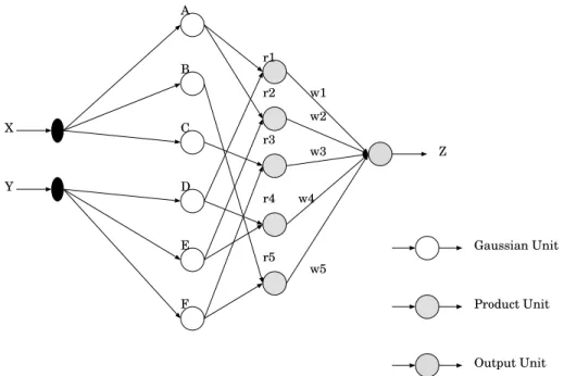
signal, and to the architecture proposed by Tresp et al. [79]. Figure 1 describes the basic network topology.
X Y A B C D E F r1 r2 r3 r4 r5 Z w1 w2 w3 w4 w5 Gaussian Unit Product Unit Output Unit
Fig. 1. Reference F–RBFN architecture. The first layer hidden units have a one–dimensional Gaussian activation function. The second layer hidden units com-pose the input values using arithmetic product. An average sum unit performs the weighted sum of the activation values received from the product units.
The activation function used in an F-RBFN with n input units is defined as the product of n one–dimensional radial functions, each one associated to one of the input features. Therefore an F-RBFN can be described as a network with two hidden layers. The neurons in the first hidden layer are feature de-tectors, each associated to a single one–dimensional activation function and are connected to a single input only. For example, if we choose to use Gaus-sian functions, the neuron rij (the i-th component of the j-th activation area)
computes the output:
µij = e − ³Ii−Cij σij ´2 (13) The neurons in the second hidden layer simply compute a product and con-struct multi-dimensional radial functions:
rj =
Y
i
µij = ej (14)
where ej was introduced in section 2.1.
Finally, the output neuron combines the contributions of the composite func-tions computed in the second hidden layer. In this architecture, a choice of
four different activation functions is possible for the output unit, in order to adapt the network to different needs. The output function can be a weighted sum
Y =X
j
wjrj (15)
The same function can be followed by a sigmoid when the network is used for a classification task. Using this function the network tends to produce an output value close to ’0’ everywhere the input vector falls in a point of the domain which is far from every activation area. The consequence is under-generalization in the classification tasks.
This problem can be avoided by introducing a normalization term in the out-put activation function:
ˆ Y = P jwjrj P jrj (16) This function is frequently used for fuzzy controller architectures [6]. In this case, one obtains a network biased toward over-generalization in a similar way as for the multi-layer perceptron. Depending on the application, under-generalization or over-under-generalization can be preferable. It is straightforward to note that equations 15 and 16 correspond to 1 and 2 respectively.
8.2.0.12 Concluding Remarks. Traditionally fuzzy controllers were de-signed by hand, expressing the domain knowledge in a set of fuzzy rules. When the membership functions are differentiable, gradient descent techniques can be applied [45]. Reyneri [70] introduced the Weighted RBFNs as a general paradigm for covering a wider set of neuro-fuzzy system. Fuzzy logic has been widely used in medical domains. RBFNs are a viable way to combine training and comprehensibility of the fuzzy rules (for an example of an application in bioengineering see [46]). In the Melanoma diagnosis scenario fuzzy con-ceptssuch as ”black dots” or ”pseudopodus” or ”dominant color” could be defined and provided to the network. Alternatively linguistic variables corre-sponding to the memberships can be discovered by the learning procedures.
9 Symbolic Interpretation of RBFNs
An important property, directly related to the fuzzy controller interpretation of the F–RBFNs is the possibility of giving an immediate, symbolic interpre-tation of the hidden neuron semantics [11,79,80]. In fact, the closed regions corresponding to neuron activation areas can be labelled with a symbol and interpreted as elementary concepts. In this section we will define a straight-forward interpretation in terms of propositional logics following [11].
x y
1 3
1.2 2.3
Activation area A(r) of neuron "r"
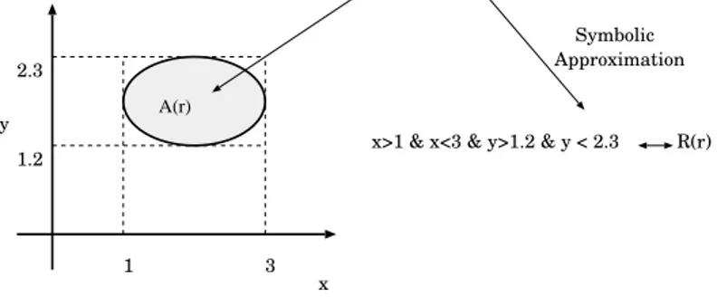
x>1 & x<3 & y>1.2 & y < 2.3 R(r) Symbolic Approximation A(r)
Fig. 2. The closed region where a factorizable radial function is dominant can be roughly approximated using a conjunctive logical assertion.
Factorized RBFNs have an immediate symbolic interpretation. In fact, defin-ing the activation area Aj of a neuron rj as the region in the input domain
where the output of rj is greater than a given threshold T, we obtain an
el-lipse with the axis parallel to the input features. Moreover, Aj is inscribed
into a rectangle Rj having the edges parallel to the input features (see
Fig-ure 2). Then, every edge rij of Rj can be seen as a pair of conditions on the
input Ii and then the whole rectangle can be read as a conjunctive condition
on the input. A variant of this symbolic interpretation, could be to assign a symbol to every edge, interpreted as an atomic proposition. In this way, the one–dimensional activation functions can be seen as a ”fuzzy” semantics of the atomic propositions. Finally, links from the second hidden layer to the output neuron can be seen as implication rule of the type:
Rj → wj (17)
being Rj the logical description of the rectangle Rj. In other words, the
mean-ing of (17) is: ”if conditions Rj hold then the value of the output is wj”. Then,
the activation function associated with the output neuron implements a kind of evidential reasoning taking into account the different pieces of evidence coming from the rules encoded in the network.
Therefore, mapping such a theory into the network structure of Figure 1, is immediate according to the fuzzy interpretation we established in the previous section. The antecedent of a rule Ri will be represented by a proper set of
neurons in the first hidden layer and by a single neuron in the second one, connected to the output neuron, representing class H. The weight on the link will be set to the numeric value (say 1) representing the concept of ”true”, if the rule is a positive one (implies H) or to the numeric value representing the ”false” (say 0 or -1) if the rule is a negative one (i.e implies ¬H).
Using activation functions having a value greater than zero on the whole do-main D, such as Gaussians do, the choice between a nonnormalized weighted sum function (equations 15or 1) and a normalized weighted sum function
(equations 16 or 2) for the output neuron is not so obvious and deserves some more attention. In logics, it is quite common to assume the Closed World Assumption (CWA) so that, anything which is not explicitly asserted is as-sumed to be false. Under this assumption, a classification theory can contain only positive rules, because the negation of a class follows from the CWA. If a nonnormalized weighted sum function (equations 15 or 1) is used, the CWA can be automatically embedded in the network semantics by using a threshold function (a sigmoid in our case) in order to split the output co–domain into two regions: one, above the threshold where the output value is high and the target class is asserted, and another, below the threshold, where the output value is low and the class is negated. As a consequence we can only model positive rules on the network. On the contrary, using a normalized weighted sum function (equations 16 or 2) the output value tends to always be ”1”, if the theory contains only positive rules, because of the normalization factor. Then, the CWA doesn’t hold anymore and negative rules must be explicitly inserted in the network in order to cover the whole domain D either with a positive or with a negative rule.
The considered F-RBFN architecture is able to approximate continuous func-tions as well as classification funcfunc-tions and, also in this case, it is possible to give them a qualitative symbolic interpretation, as is done for fuzzy controllers. In this case, both nonnormalize and normalize weighted sum function can be used for the output neuron.
9.0.0.13 Concluding Remarks. The symbolic interpretation of an RBFN allows a wide range of symbolic learning algorithms to be applied in order to initialize the basis functions. Decision trees [17] or symbolic induction systems such as SMART+ [15] can be used to construct the layout from a sample set of data. Alternatively, if domain knowledge is available, e.g. from an expert, it can be directly inserted into the network. Gradient descent provides a technique for refining knowledge with data. Finally, it is possible to exploit symbolic semantics for mapping knowledge back (for an example in a prognosis domain see [11]). For an extension of this property to first-order logics see [16]. Sym-bolic interpretation permits to map, refine and extract knowledge in terms of rules. The comprehensibility of the rules can be an advantage for the validation and acceptatance of a system in medical domains. In the melanoma diagnosis scenario the ABCD rules used by the dermatologists could be inserted and refined in the network. Activated rules can be prompted as an explanation.
10 A Statistical Approach to RBFNs
The architecture of the RBFNs presents a strong similarity with regression techniques, based on non–parametric estimation of an unknown density func-tion [75] and with the Probabilistic Neural Networks [76,77].
10.1 Kernel Regression Estimators
This method is known as kernel regression. The basic idea is that an un-known random function f (¯x) = y can be constructed by estimating the joint probability density function g(¯x, y):
f (¯x) = E(Y | ¯X = ¯x) = Z Rnyf (y|¯x)dy = R Rnyf (¯x, y)dy R Rnf (¯x, y)dy
The technique used for estimating g, is the kernel smoothing of which the Parzen windows technique is a particular case. The general form of a kernel estimator of a density function h(¯z) defined on a space Rd is:
ˆh(¯z) = 1 N |H| N X i=1 Kn+1(H−1(¯z − ¯zi))
where H is a d × d nonsingular matrix and Kd : Rd → R is a multivariate
kernel density that satisfies the conditions: Z RdKd( ¯w)d ¯w = 1d Z RdwK¯ d( ¯w)d ¯w = 0d Z Rdw ¯¯w TK d( ¯w)d ¯w = Id
The constant N is the number of kernels that in the statistical literature usually coincides with the number of examples.
Let us consider ¯z = (¯x, y) and a product kernel of the form
The estimation of g becomes: ˆ g(¯x, y) = 1 N |Hx|hy N X i=1 Kn(Hx−1(¯x − ¯xi))K1(h−1y (y − yi)) Remembering that 1 hy Z RnK1(h −1 y (y − yi))dy = 1 1 hy Z RnyK1(h −1 y (y − yi))dy = yi
and substituting the estimate of g in the denominator and numerator of the (10.1) Z Rnf (¯x, y)dy = 1 N |Hx|hy N X i=1 Kn(H −1 x (¯x − ¯xi)) Z RnK1(h −1 y (y − yi))dy = 1 N |Hx| N X i=1 Kn(H −1 x (¯x − ¯xi)) Z Rnyf (¯x, y)dy = 1 N |Hx| N X i=1 yiKn(H −1 x (¯x − ¯xi))
finally we obtain the approximation of the f :
ˆ f (¯x) = PN i=1yiKn(Hx−1(¯x − ¯xi)) PN i=1Kn(Hx−1(¯x − ¯xi)) (18) In the univariate case the (18) is called Nadaraya-Watson Estimator. It is easy to see by comparing the equation (18) to the normalized RBFN;
N (x) = Pn
i=1wiei(k x − ci k)
Pn
i=1ei(k x − ci k)
that this kind of network has the same structure. The only difference relies on the fact that no kernel-like conditions are usually stated on the radial functions. Among others this connection was noted by Xu et al. [87], who exploited it for extending some results of kernel estimators like consistency and convergence rate to RBFNs. An accessible description of this approach has been proposed by Figueiredo [28]. More recently Miller and Uyar [56] presented a similar result for the decision surface of the RBFN classifier. In
particular, Yee and Haykin [88] and [89] developed this interpretation for time series prediction.
10.2 Probabilistic Neural Networks
Probabilistic Neural Networks (PNN) originate in a pattern recognition frame-work as tools for building up classifiers. In that frameframe-work the examples of a classification problem are points in a continuous space and they belong to two different classes conventionally named 0 and 1. PNN were first proposed by Specht [76,77], who proposed to approximate, separately, the density distribu-tions g1(¯x) and g0(¯x) of the two classes and use a Bayes strategy for predicting
the class. ˆ f (¯x) = 1 if p1l1g1(¯x) > p0l0g0(¯x) 0 if p1l1g1(¯x) < p0l0g0(¯x)
where p1 and p0 are the a priori probabilities for the classes to separate and l1
and l0 are the losses associated with their misclassification (l1 loss associated
with the decision ˆf (¯x) = 0 when f (¯x) = 1).
Then the decision surface is described by the equation: g1(¯x) = kg0(¯x)
where,
k = p0l0 p1l1
and defining σ(x) as a threshold function the estimate of the target function is:
ˆ
f (¯x) = σ(g1(¯x) − kg0(¯x))
Again the density approximations are made using the kernel estimations g1(¯x) = 1 N1|H| N1 X i=1 Kn+1(H −1 (¯z − ¯zi))
with the extension of the sum limited to the N1 instances belonging to class
1 and analogously for the class 0. ˆ f (¯x) = σ( 1 |H| N X i=1 C(zi)Kn+1(H −1(¯z − ¯z i)) (19) where, C(zi) = 1 if f (zi) = 1 −kN1 N0 if f (zi) = 0
The equation (19) is a particular case of the RBFN described in equation 2 for approximating boolean functions.
10.2.0.14 Concluding Remarks. In the statistical framework it is com-mon to use all the data as centres of the kernels. In the case of a large data set it is possible to limit the initialization to an extracted sample of data. It is worth noting, that no computation is needed to find the values of the weights. In fact, as an effect of the normalization terms contained in the kernels, the weights are equal to the output values, or set to an estimate of the a priori probability of the class. This method can be applied in an incremental way, but like any other method which uses all the data, it suffers for the overgrowing of the approximator. This property permits to analyse directly the network in terms of probability having a direct statistical interpretation. In fact, given the estimation of the density implicitly formed by the RBFN is possible es-timate all the statistics parameter of the distribution. Moreover exploiting a factorizable architecture is possible to express independency between the in-puts as is normally done in Bayesian Networks. Probabilistic interpretation is important in a medical domain. Performance of the network can be evaluated with respect to the known statistics of the diseases. In the Melanoma diag-nosis scenario the conditional probabilities of the malignant outcome given a variable, e.g. age, can be showed validating the model.
11 RBFNs as Instance–Based Learners
Instance–based learning or lazy learning can be defined as a learning method that delays some, or even all, the computation efforts until the prediction phase, limiting the learning to the simple memorization of samples (see [57]). Since little or no computation at all is done during the learning phase, the approach is suitable for on–line learning. Some of the most used algorithms in this context, are the well-known, k–Nearest Neighbour family. During the pre-diction phase, the computation of a distance defined on the input space, leads
to the determination of the k nearest neighbours to be used for predicting the value of the target variable. RBFNs can be viewed as a particular k-NN with k = n number of the basis function and a local distance function defined by e(k ¯x − ¯xi k). In this framework, training the network can be interpreted
as the determination of the n local metrics, associated to the centres of the basis functions. Moreover, RBFN centres can be viewed as instances of the unknown function, in fact the earlier proposal of the RBFN with no centre clustering was a completely instance–based approach. When the centres are determined by a training algorithm, they can be interpreted in association with the respective weight as prototypes of the unknown function. An ap-plication of this is the shrinking technique [48] based on the principle that centres and weights of an RBFN can be seen as pairs (ci, wi) belonging to the
space X × Y , as the examples of the target function do. Hence, they can be interpreted as prototypes of the target function and be processed by the same techniques used for the data. In particular, Katenkamp clustered the (ci, wi)
of a trained network for initializing a new smaller network. That can be useful for implementing a simple knowledge transfer between different –but similar– learning tasks. Katenkamp exploited this technique successfully on the simple cart-pole control task, transferring knowledge from tasks that differ only for the numeric values of the parameters.
11.0.0.15 Concluding Remarks. RBFNs can be considered as instance-based learners. As a consequence is possible to consider to extract the knowl-edge in terms of similar cases. Cases can be a natural way of presenting the results to a physician. In the melanoma diagnosis scenario it could be possible by inspection of the activation of the Radial Functions retrieve a similar lesion and visualize it to the user as an explanation of the outcome.
12 RBFNs as Structurally Modifiable Learners
In the sections 5-11 we noted that some of the presented methods were imme-diately suitable for working incrementally. In particular, both statistical and instance–based learning frameworks, adopt the technique of initializing the centres with the samples of the training set and performing almost no other computation during the training phase. Hence, it is straightforward to add a new function when a new sample is available. Unfortunately, as noted by Platt [67] referring to Parzen Windows and k–NN, the two mentioned algorithms present a drawback. The resulting RBFN grows linearly with the number of the samples. Platt also proposed a neural architecture, called Resource Allo-cation Networks, which combines an on–line gradient descent with a method for adding new radial functions. A new function is added when a new sample
falls far from the already existing centres, or causes an error which is greater than the average. Fritske [31] noted that RANs suffer from noise sensitivity because they add a new function for each poorly mapped sample. He therefore proposed an interesting algorithm, called GCS (see also [33]). Blanzieri and Katenkamp [12] reported that, when experimented in its original formulation, Fritske’s algorithm showed two major drawbacks. First, instead of reaching a stable structure, it indefinitely continues to alternate neuron insertions and neuron deletions, while the error rate remains quite high. Second, GCS turned out to be very keen on unlearning. Blanzieri and Katenkamp proposed an im-proved version of GCS called DCL (Dynamic Competitive Learning) which fixes the first drawback but is not yet able to avoid the unlearning problem. In order to cope with this last case, a new algorithm (Dynamic Regression Tree, DRT), which adopts a different strategy for constructing the network, has been proposed. In particular, DRT uses a more accurate strategy for in-serting new radial function so that the on-line clustering algorithm is not required. This is done by explicitly considering the symbolic interpretation (6) associated to the radial functions. When an activation area Araccumulates an
error which cannot be reduced any further by the ∆-rule, DRT split it along a dimension, using a method similar to the one used by CART [17]. In order to select the dimension and the split point, DRT keeps a window on the learning events as is done in some approaches to incremental construction of decision trees [82]. Moreover, DRT is not prone to unlearning and is somehow related to Median RBFNs proposed by [13].
A regularization–based approach to solve some of the problems of the RAN is proposed by Orr [61]. The method is named Regularization Forward Selec-tion and selects the centres among the samples of the basis funcSelec-tions, that mostly contribute to the output variance. The selection is performed in the regularization framework. Its major drawback is that the fast version of the algorithm is not suitable for on–line learning.
A completely different approach was pursued by [47], which set the problem of centres selection within the framework of functional Hilbert spaces. Intro-ducing the notion of scalar product between two basis functions, the angle they form can be used as a criterion for inserting new functions. Moreover the authors substituted the gradient descent used in the RAN with an ex-tended Kalman filter. Yee and Haykin [88] proposed also a structural update algorithm for time-varying regression function. Structural learning is also a characteristic of the neuro-fuzzy system of Kim and Kasabov [49] similar to some regard to recurrent RBFNs. Finally is necessary to cite the bayesian ap-proach proposed by Holmes and Mallick[41], the evolutionary strategy adopted by Esposito et al [27] and the competitive learning approach of [62]. The lo-cality property that permits the structural learning can be also exploited for divide-and-conquer strategies such as the decomposition technique proposed by [19]. Pruning of trained neural networks in order to get more readable rules
has been studied by Augusteijn and Shaw [3].
12.0.0.16 Concluding Remarks. The architecture of RBFNs is charac-terized by locality. As a consequence RBFNs support incremental and struc-tural dynamic algorithms in a nastruc-tural way. Unlearning can be prevented as noted again by Hamker [38]. In medical domains, it is common to have a grow-ing number of cases [60]. In the melanoma diagnosis scenario the low number of malignant lesions suggest that an incremental algorithm can be useful.
13 The Melanoma Diagnosis Scenario Revised
The melanoma diagnosis scenario introduced in section 1 has been used through-out the paper in order to illustrate the potential advantages of the different way of interpreting RBFNs. In this section we revise and discuss systematically those potential advantages posing them in a more general perspective.
In the melanoma diagnosis scenario a dermatologist that uses a D-ELM device is supported in her diagnostic activity of this potential fatal skin lesion. A complete illustration of the applicative scenario is reported in [73]. Here we emphasize the following points:
• The misclassification costs is an issue: false negative are far worse than false positives (sensitivity and specificity and ROC curves are introduced for measuring the performance);
• The input is hybrid: D-ELM image and clinical information;
• Knowledge is available from dermatology literature (ABCD rules and qual-itative concepts as Black dots and pseudopods;
• Comprehension of the result is an issue; • Datasets are small.
Some interpretations of RBFNs have been already exploited for melanoma diagnosis, others are potential. RBFN’s can be considered as Neural Networks (Section 4) and we have already noted that this appears to be the most com-mon use of the RBFNs in medical application. This is also the case for the Melanoma Diagnosis scenario (see references in [10]). Considering RBFNs as Regularization Networks (Section 5) is important because it sets a differential contraint on the approximating function. Regularization could be explored in order to enhance the performance. However, cost-sensitiveness has to be con-sidered. RBFNs considered as Supported Vector Machines (Section 6) were where used in [71] for the task of diagnosis of pigmented skin lesions. More-over, theoretical bounds on the generalization error can improve confidence in
the system and its chances of acceptance. Section 7 shows that Wavelets Net-works can be seen as particular RBFNs In the melanoma diagnosis scenario wavelets could be used to elaborate the D-ELM images so RBFNs can provide a common framework for signal related features and clinical features. More in general, Regularization Theory, SVM and WAVELETS approaches share the feature of fixing a property of the approximator: a differential property, a generalization property and a spectral property respectively.
Considering RBFNs as fuzzy systems leads to their symbolic interpretation (Sections 8 and 9). Fuzzy concepts such as ”black dots” or ”pseudopodus” or ”dominant color” could be defined and provided to the network. Alternatively, linguistic variables corresponding to the memberships can be discovered by the learning procedures. The ABCD rules elaborated by the dermatologists could be inserted and refined in the network. Moreover, activated rules can be prompted as an explanation. More in general, RBFNs are knowledge-based neural system.
The statistical approach to RBFNs leads to a probabilistic interpretation (Sec-tion 10) that is particularly important in a medical domain. Performance of the network can be evaluated with respect to the known risk statistics of the dis-eases. The conditional probabilities of the malignant outcome given a variable, e.g. age, can be naturally computed and showed to an expert for validation. Seeing RBFNs as a type of Instance Based Learning (Section 11) suggests to use the activation of the Radial Functions for retrieving and returning a sim-ilar lesion as an explanation of the outcome. More in general, RBFN shares with kernel-regression methods the nice property of representing a model of the data (the regressor, namely the RBFN) and a set of samples/prototypes.
Finally, RBFNs naturally support learning algorithms with structural changes (Section 12). In the melanoma diagnosis scenario the low number of malignant lesions suggest that an incremental algorithm can be useful. A growing set of cases can be exploited in order to provide a better performance. More in general, the locality of the approximation strategy of the RBFN allows for structural online learning.
It is worth noting that the cost-sensitive requirements of the melanoma diag-nosis scenario do not seem to be met by RBFNs. In fact, at the best knowledge of the author, cost-sensitive learning for RBFNs has not been systematically addressed yet. However, cost-sensitiveness is an open issue, for instance, in SVM research, so, given the SVM intepretation, the results can be transferred to a subclass of RBFNs. In this way it is possible to exploit different properties depending on the characteristics of the application
14 Conclusions
This paper is concerned with Radial Basis Function Networks (RBFNs) and it addresses their different interpretations and the applicative perspectives that those interpretations suggest using as example a melanoma diagnosis scenario. We have introduced the feed–forward version of the network and placed it in the framework of function approximation problems. From the technical point of view, we have presented the basic architecture of the RBFNs as well as the different approaches (Artificial Neural Networks, Regularization Theory, Support Vector Machines, Wavelet Networks, Fuzzy Controllers, Symbolic In-terpretation, Statistical Approach, Instanced Based Learning) and their corre-spondent learning algorithms. After having introduced the distinction between static and dynamic algorithms we completed the work presenting a brief sur-vey of the latter.
An important point of the present work is the systematic way the differ-ent interpretations has been presdiffer-ented in order to permit their comparison. RBFNs are particularly suitable for integrating the symbolic and connectionist paradigms in the line draw by Towell and Shavlik [78] whose recent develop-ments has been surveyed by Cloete and Zurada [22]. This symbolic interpreta-tion permits to consider RBFNs as intrinsically Knowledge-Based Networks. Moreover, RBFN have also very different interpretations. They are Regular-ization Networks so there is the possibility of tuning the regularRegular-ization param-eter. They are Support Vector Machines so they gain theoretical foundation from statistical learning theory. They are related to Wavelet Networks so they can gain advantage in signal applications such as ECG. They have a Fuzzy interpretation so they can be interpreted in terms of fuzzy logic. They have a statistical interpretation so they can produce, after training, knowledge in terms of probability. They are also Instance-Based learners and so they can provide a case-based reasoning modality. Finally, another basic property of the RBFN is the locality that permits the synthesis of incremental dynamic algorithms permitting the growing of the cases without unlearning.
From the ponit of view of medical application the potential of the RBFN archi-tecture is not yet been exploited completely. In fact, given the interpretations and properties described above it is possible to tailor in a very flexible way applications that exploit two or more of the properties.
References
[1] A.S. al Fahoum and I. Howitt. Combined wavelet transformation and radial basis neural networks for classifying life-threatening cardiac arrhythmias.