Optimisation of artificial neural networks for predicting fish assemblages in rivers

Lek · Scardi · Verdonschot · Descy · Park (Eds.)

Modelling Community Structure

in Freshwater Ecosystems

The book presents approaches and methodologies for

predicting the structure and diversity of key aquatic

communities (namely diatoms, benthic

macroinverte-brates and fish), under natural conditions and under

man-made disturbance. Such an approach will make it

possible to: 1) set up procedures for robust and sensitive

ecosystem evaluation, based on the prediction of the

expected community structure; 2) model community

structure in disturbed ecosystems, taking into account

all the relevant ecological variables; 3) test ecosystem

sensitivity to natural and anthropic disturbance; and

4) explore specific actions to be taken for the restoration

of ecosystem integrity.

123

1

isbn

3-540-23940-5

Le

k · Scar

di ·

V

er

do

nscho

t

y · P

ar

k (E

ds.)

Modelling Community

Structure

in Freshwater

Ecosystems

Modelling C

ommunity Struc

ture

in F

reshw

a

ter E

cosy

st

ems

Sovan Lek

Michele Scardi

Piet F.M. Verdonschot

Jean-Pierre Descy

Young-Seuk Park

Editors

›

springeronline.com

Modelling Community

Structure

in Freshwater

Ecosystems

8 Optimisation of artificial neural networks for predicting

fish assemblages in rivers

Scardi M.

*

, Cataudella S.

, Ciccotti E.

, Di Dato P.

, Maio G.

,

Marcona-to E.

, Salviati S.

, Tancioni L.

, Turin P.

, Zanetti M.

Predicting the structure of fish assemblages in rivers is a very important goal in

ecological research, both from a purely theoretical point of view and from an

ap-plied one. Moreover, it will play a relevant role in the definition of reference

con-ditions in the light of the EU Directive 2000/60/EC (i.e. the Water Framework

Di-rective). Estimates of the probability of presence/absence of fish species have been

obtained so far using different approaches. Although conventional statistical tools

(e.g. logistic regression) provided interesting results, the application of artificial

neural networks (ANNs) has recently outperformed those techniques. ANNs are

especially effective in reproducing the complex, non-linear relationships that link

environmental variables to fish species presence and/or abundance. In this chapter

some new developments in ANN training procedures will be presented, which are

specifically aimed at solving ecological problems related to the way the errors are

computed in species composition models. The resulting improvements in species

prediction involve not only the accuracy of the models, but also their ecological

consistency. A case history about fish assemblages in the rivers of the Veneto

re-gion (NE Italy) is presented to demonstrate how the enhanced modelling strategy

improved the accuracy of the predictions about fish assemblages.

Keywords: predictive modelling, fish assemblage, error back-propagation,

multilayer perceptron, artificial neural network training.

8.1 Introduction

Fish assemblages are among the most sensitive and reliable indicators of the

eco-logical status of stream and rivers (Fausch et al., 1990). Fish assemblages are able

to integrate over both time and space the biological response to ecological

proc-esses more effectively than other biotic components (Harris, 1995). Sampling fish

fauna, of course, is not as simple as sampling other organisms, but in spite of this

problem indices of biotic integrity based on fish have been developed and are now

1 Department of Biology, University of Rome “Tor Vergata”, Via della Ricerca Scientifica, 00133 Rome, Italy

* Corresponding author: mscardi@mclink.it

2 Aquaprogram s.r.l., Via Borella 53, 36100 Vicenza, Italy 3 Bioprogramm s.c.r.l., Via Tre Garofani 36, 35124 Padova, Italy

widely accepted (Karr, 1981; Karr et al., 1986). Targeting fish fauna in

environ-mental monitoring activities is effective not only from the ecological point of

view, but also in the light of the need for straightforward communication with

de-cision-makers as well as with other stakeholders. In fact, fish are probably the

most direct and intuitive expression of aquatic ecosystem quality (McCormick et

al., 2000).

Therefore, it is not surprising that composition, abundance and age structure of

fish fauna are considered as some of the main biological quality elements for the

classification of ecological status of surface water in the EU Water Framework

Di-rective (i.e. DiDi-rective 2000/60/EC of the European Parliament and of the Council

of 23 October 2000 establishing a framework for Community action in the field of

water policy).

The above-mentioned Directive also states that biological reference conditions

have to be established for each type of water body. These reference conditions are

based on community structure and take into account all the biological quality

ele-ments, thus including fish fauna as well as benthic macroinvertebrates and aquatic

flora. Hence, modeling fish assemblage composition on the basis of biotic and

abiotic environmental descriptors will play a major role in the implementation of

the Water Framework Directive and, more in general, in the management of

aquatic ecosystems.

Predicting fish fauna as well as other biotic assemblages is not only relevant to

the definition of reference conditions that are aimed at the evaluation of

environ-mental quality. In fact, it is also an important achievement in scientific research,

e.g. as a framework for studies on species interactions, and it can be very useful

for a number of other applied tasks. In particular, species composition models may

support environmental management by simulating different environmental

scenar-ios and pointing out the most critical factors that need changes or regulation.

Sen-sitivity analyses of the species composition models play a relevant role in this kind

of studies.

Even though the idea of modeling fish fauna composition on the basis of

envi-ronmental variables is not new (e.g. Faush et al., 1988), only recently Artificial

Neural Networks (ANNs) have been applied to this problem. ANNs have been

used to predict fish species richness (e.g. Guegan et al., 1998) as well as density

and biomass of single fish populations (Baran et al., 1996; Lek et al., 1996a,b;

Mastrorillo et al., 1997) and ecological characteristics of fish assemblages

(Agui-lar Ibarra et al., 2003). As far as fish assemblages composition at river basin scale

is considered, only a few models have been developed so far, either using

conven-tional statistical methods (e.g. Oberdorff et al., 2001) or ANNs (Boët and Fhus,

2000; Joy and Death, this volume; Olden and Jackson, 2001). A very useful

intro-duction to the ecological applications of ANNs can be found in Lek and Guégan

(1999).

ANNs and other modelling techniques that have been developed and formerly

applied in other disciplines have been often introduced into ecological applications

with no modification. In most cases this was not a problem and very useful results

were obtained anyway. However, in ecological modelling adaptations of the

mod-elling techniques are sometimes required in order to fit particular needs or to

properly exploit the available information. This is certainly the case of species

composition models, as the data that are involved in this kind of application

can-not be regarded as mere numbers, because each species has a different ecological

“meaning”, which in turn depends on its coenotic context.

This chapter will present a case study about fish assemblages from some river

basins in north-eastern Italy, showing how the above-mentioned problem can be

tackled by developing ecologically enhanced ANNs.

8.2 Data set

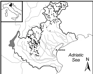
The ANN models presented in this study are based on a data set that included

sampling sites from several river basins in the Veneto region (north-eastern Italy),

as shown in Fig. 3.8.1. The data set consisted of 264 records and it comprised two

groups of variables. The first group included the variables to be predicted by the

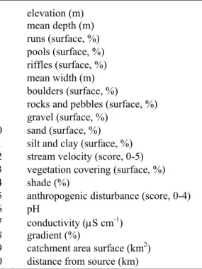
models, i.e. 34 fish species, whereas the second group embraced 20 predictive

en-vironmental variables, as shown in Tables 3.8.1 and 3.8.2 respectively.

Venice

Adriatic

Sea

Figure 3.8.1 The sampling sites (black dots) were located in several river basins

in the Veneto region (NE Italy).

Fish has been collected by means of electrofishing gear. Either direct current or

pulsed direct current electrofishing devices have been used in streams and small

rivers, while these tools were supported by nets when only part of larger rivers

was sampled. Basically, in the latter case the electrofishing area was closed by

means of nets that also acted as a sampling device.

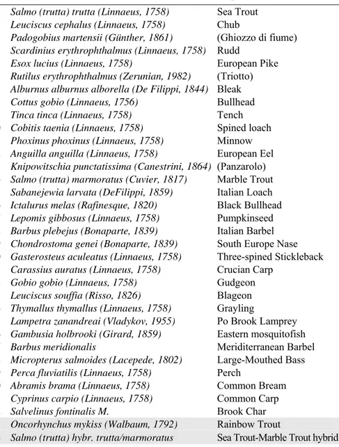
Table 3.8.1 List of the fish species in the Veneto data set. Modeled species are on

white background, while species that were excluded (see text) are on grey

background. Italian names are shown in parentheses for those species that do not

have an English name.

n Scientific name

English name

1

Salmo (trutta) trutta (Linnaeus, 1758)

Sea Trout

2

Leuciscus cephalus (Linnaeus, 1758)

Chub

3

Padogobius martensii (Günther, 1861)

(Ghiozzo di fiume)

4

Scardinius erythrophthalmus (Linnaeus, 1758) Rudd

5

Esox lucius (Linnaeus, 1758)

European Pike

6

Rutilus erythrophthalmus (Zerunian, 1982)

(Triotto)

7

Alburnus alburnus alborella (De Filippi, 1844) Bleak

8

Cottus gobio (Linnaeus, 1756)

Bullhead

9

Tinca tinca (Linnaeus, 1758)

Tench

10 Cobitis taenia (Linnaeus, 1758)

Spined loach

11 Phoxinus phoxinus (Linnaeus, 1758)

Minnow

12 Anguilla anguilla (Linnaeus, 1758)

European Eel

13 Knipowitschia punctatissima (Canestrini, 1864) (Panzarolo)

14 Salmo (trutta) marmoratus (Cuvier, 1817)

Marble Trout

15 Sabanejewia larvata (DeFilippi, 1859)

Italian Loach

16 Ictalurus melas (Rafinesque, 1820)

Black Bullhead

17 Lepomis gibbosus (Linnaeus, 1758)

Pumpkinseed

18 Barbus plebejus (Bonaparte, 1839)

Italian Barbel

19 Chondrostoma genei (Bonaparte, 1839)

South Europe Nase

20 Gasterosteus aculeatus (Linnaeus, 1758)

Three-spined Stickleback

21 Carassius auratus (Linnaeus, 1758)

Crucian Carp

22 Gobio gobio (Linnaeus, 1758)

Gudgeon

23 Leuciscus souffia (Risso, 1826)

Blageon

24 Thymallus thymallus (Linnaeus, 1758)

Grayling

25 Lampetra zanandreai (Vladykov, 1955)

Po Brook Lamprey

26 Gambusia holbrooki (Girard, 1859)

Eastern mosquitofish

27 Barbus meridionalis

Meriditerranean Barbel

28 Micropterus salmoides (Lacepede, 1802)

Large-Mouthed Bass

29 Perca fluviatilis (Linnaeus, 1758)

Perch

30 Abramis brama (Linnaeus, 1758)

Common Bream

31 Cyprinus carpio (Linnaeus, 1758)

Common Carp

32 Salvelinus fontinalis M.

Brook Char

33 Oncorhynchus mykiss (Walbaum, 1792)

Rainbow Trout

Two fish taxa, namely Oncorhynchus mykiss, i.e. the rainbow trout, and Salmo

(trutta) hybr. trutta/marmoratus, i.e. a sea trout - marble trout hybrid (on grey

background in Table 3.8.1), were excluded from the models, as their distribution

only partly depends on environmental variables. In fact, the distribution of the first

taxon is linked to the artificial release of reared juveniles, while the second taxon

one is clearly not independent of the distribution of the two parent species and is

probably associated to problems in species identification too.

Some of the available records refer to sampling activities that were carried out

at the same site at two different times, thus representing the local interannual

vari-ability of both the fish fauna and the environmental variables.

The fish fauna composition was described using binary variables, i.e. presence

or absence of each taxon. Quantitative data, although available in most cases, were

not considered for model development as they were not enough accurate because

of the combined effects of varying efficiency of the electrofihing gear and

mor-phodynamic heterogeneity of the sampling sites. The environmental variables

were coded in different ways, either as quantitative or semi-quantitative data, and

all the non-binary variables were normalized by rescaling them in the [0,1]

inter-val.

Table 3.8.2 Environmental descriptors used as input (i.e. predictive) variables in

the models.

1 elevation

(m)

2 mean

depth

(m)

3

runs (surface, %)

4

pools (surface, %)

5 riffles

(surface,

%)

6 mean

width

(m)

7 boulders

(surface,

%)

8

rocks and pebbles (surface, %)

9

gravel (surface, %)

10 sand

(surface,

%)

11

silt and clay (surface, %)

12

stream velocity (score, 0-5)

13

vegetation covering (surface, %)

14 shade

(%)

15

anthropogenic disturbance (score, 0-4)

16 pH

17

conductivity (µS cm

₎

18 gradient

(%)

19

catchment area surface (km

₎

The whole data set was divided into three subsets for training, validating and

testing the ANN models. The training data set included 50% of the records

(n=132), whereas both the validation and the test data sets included 25% of the

re-cords each (n=66). Each record was assigned to a different subset after sorting all

the records according to the elevation of the sampling sites. Starting from the

highest elevation, the records were divided into the above-mentioned subsets by

assigning uneven records to the training subset and by assigning each couple of

successive even records to the validation and test subset, respectively. This way

the records in each group of four were assigned to the (1x) training, (2x)

valida-tion, (3x) training and (4x) test data subset, with x ranging from 1 to 66. This break

up strategy allowed a homogeneous allocation of records for different elevations

classes among the three subsets, thus stratifying the procedure on the basis of the

most relevant environmental variable.

8.3 Neural network training

The most common type of ANN, i.e. the multilayer perceptron, was used for

mod-eling the fish fauna composition. The error back-propagation algorithm

(Rumel-hart et al., 1986) was used for training the ANNs, both in its original formulation

and in a modified version that will be described later in this chapter. Other training

algorithms were not tested because the theoretical advantages they might provide

(e.g. quicker training) are not really relevant for ecological applications.

ANNs with 20 input nodes, 32 output nodes and 17 nodes in the hidden layer

were selected after a set of empirical tests involving ANNs with different numbers

of nodes in the hidden layer (from 10 to 40 nodes). The selected architecture was

the one that provided the minimum overall error with respect to an independent

test set. However, the selection of the number of nodes in the hidden layer was not

a critical issue, as the differences among the models were negligible. Sigmoid

ac-tivation functions [i.e. f(x)=1/(1-e

_{)] were used both in the hidden and in the}

out-put nodes of all the ANNs that have been trained and used in this study.

In order to prevent overtraining, i.e. to avoid that the ANN “learned by heart”

the fish fauna composition at each known site while loosing its generalization

abil-ity, different strategies were adopted. The first strategy involved an early stopping

of the training procedure. In other words, the training procedure was terminated as

soon as the error, computed on the basis of the validation set only, ceased to

de-crease monotonically (obviously, the validation set records were never used as

training patterns). The second strategy was based on the random selection of a

subset of training patterns at each epoch during the training procedure. This way it

was not possible for the ANN to be influenced by the order in which the training

patterns were submitted (thus possibly memorizing them). Finally, white noise in

the [-0.01,0.01] range was added to each input, i.e. predictive variable. Such a

small random perturbation of the input values, also known as jittering, favored the

generalization of an ANN model because the latter learned how to associate each

output pattern with a set of input intervals rather than with a single input pattern

(Györgyi 1990).

The accuracy of the ANN predictions was expressed by the percentage of

Cor-rectly Classified Instances (CCI), while the significance of the deviation of the

ANN predictions from a random model was tested by means of the K statistics

(Cohen, 1960; Fielding and Bell, 1997). Details about the computation of CCI

percentage and K statistics are provided in the Appendix.

8.4 Model selection

A few different basic options are available for developing models of species

dis-tribution using ANNs. The first option is to train a different model for each

spe-cies, whereas the other is to train a single model that is able to simultaneously

pre-dict the distribution of all the species. Another option is to split the species list into

two or more subsets on the basis, e.g. of trophic characteristics, and to train a

model for each subset. In the latter case, however, the number of possible models

is very high and selecting the best combination is not a straightforward task.

If only the first two options are considered, the selection of the best approach

may be based on empirical tests, but there are also some theoretical consideration

that should be taken into account.

In fact, when modeling the distribution of a complex set of species, as a fish

as-semblage, an ANN model that predicts more than a single species is able to learn

not only the distribution of each species, but also some information about

interac-tions among species. Of course, ecologists know that this kind of information is

relevant, but in many cases their theoretical knowledge about species interactions

is not adequate, as it is often based on hypotheses, personal observations, etc.

Therefore, it is not easy to exploit such knowledge in modeling applications using

conventional statistical methods (e.g. logistic regression). Since ANNs are able to

learn from data, they are also able to learn by themselves what is relevant in

spe-cies interactions and this may enhance their predictive ability.

Given a species assemblage containing s species, 2

_{different combinations of}

species presence and absence data exist. In the case of our data set,

2

_{=4294967296 different patterns are theoretically possible, but only 131}

differ-ent patterns were actually found in 264 observations. This is clear evidence for the

non-independence of different species responses to environmental factors and for

the role that biotic interactions play.

Even though simultaneously modeling all the species in a community or in an

assemblage is theoretically more efficient, there are practical constraints that may

hinder this approach. In fact, the complexity of the ANN structure grows very

rap-idly with the number of species to be modeled, and the need for training data

grows proportionally. Moreover, the set of predictive environmental variables

used by the model might be more relevant to some species then to others, and this

would impair the model response. In the case of fish assemblages, however, the

overall number of species is usually not too large and the species response to

envi-ronmental variables is rather homogeneous. Therefore, a single model approach

was selected in our study.

8.5 A conventional training procedure

The first attempt at modeling the fish assemblage was based on a very

conven-tional ANN approach, as a 20-17-32 multilayer perceptron was trained using an

ordinary error back-propagation algorithm. This ANN was able to predict the

presence of all the species on the basis of environmental variables. The output

values it returned ranged in the [0,1] interval and therefore they could be regarded

as the probability for each species of being observed. The predicted fish

assem-blage composition was then obtained by setting a 0.5 threshold for each output,

thus converting the continuous output values into binary values (i.e. species

pres-ence or abspres-ence estimates) by means of a process that is closely related to

defuz-zyfication.

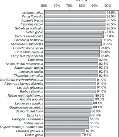
The overall accuracy of the ANN model was very good, as the CCI ranged

from 98.5% to 79.1% (Fig. 3.8.2), while the average percentage of CCI was

91.6%.

Figure 3.8.2 Percentages of Correctly Classified Instances (CCI) for the 32

The percentage of CCI, although very convenient and easy to compute, is

sometimes a misleading criterion for evaluating the ability of a model to predict

species composition. In fact, it would be really appropriate in case the number of

presence records for a given species is exactly the same as the number of absence

records, and it would still be acceptable in case the ratio between presence and

ab-sence records is not too far from one. On the contrary, when the ratio becomes too

small (or too large), an ANN model can be easily affected by a significant bias.

For instance, when very rare species are modeled, an ANN that always returns

null outputs can easily provide a very high CCI percentage. In other words, if a

species were present in 2 out of 100 records (i.e. if its frequency were 2%), an

ANN would be very easily able to provide 98% of CCI by constantly predicting

the absence of that species. Needless to say, notwithstanding a very high CCI

per-centage, such an ANN could not be considered as a true model.

Therefore, another procedure was selected for evaluating the accuracy of the

ANN model in the light of the actual frequency of presence or absence record for

each species. In particular, the K statistics (Cohen, 1960; Fielding and Bell, 1997)

was applied in order to test whether the predictions for each species were

signifi-cantly different from those of a random model or not. The ANN model was able to

effectively predict 20 species out of 32, i.e. in 20 cases the K statistics was

signifi-cantly different from zero (p=0.95), whereas it failed in the remaining cases (table

3.8.3).

It was evident, however, that the ability of the ANN to predict species presence

and absence was strictly related to species frequency. In fact, the maximum

fre-quency among the 12 species with non-significant K statistics was 8.71%, and 10

of them had frequencies lower than 5%. Thus, the model failed in predicting

sev-eral rare species, while it was quite accurate in predicting more frequent species

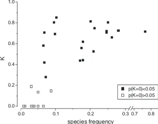
(Fig. 3.8.3).

Figure 3.8.3 Conventional ANN model: K statistics vs. species frequency. The

model is not reliable as far as rare species are concerned, whereas it works much

better with more frequent species.

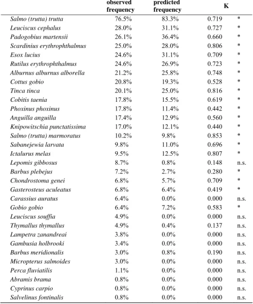
Table 3.8.3 Conventional ANN model: observed and predicted frequency by

spe-cies (sorted in descending order of observed frequency) and K statistics

(signifi-cant values are marked with asterisks).

observed frequency

predicted

frequency K

Salmo (trutta) trutta 76.5% 83.3% 0.719 * Leuciscus cephalus 28.0% 31.1% 0.727 * Padogobius martensii 26.1% 36.4% 0.660 * Scardinius erythrophthalmus 25.0% 28.0% 0.806 * Esox lucius 24.6% 31.1% 0.709 * Rutilus erythrophthalmus 24.6% 26.9% 0.723 * Alburnus alburnus alborella 21.2% 25.8% 0.748 * Cottus gobio 20.8% 19.3% 0.528 * Tinca tinca 20.1% 25.0% 0.816 * Cobitis taenia 17.8% 15.5% 0.619 * Phoxinus phoxinus 17.8% 11.4% 0.442 * Anguilla anguilla 17.4% 12.9% 0.560 * Knipowitschia punctatissima 17.0% 12.1% 0.440 * Salmo (trutta) marmoratus 10.2% 9.8% 0.853 * Sabanejewia larvata 9.8% 11.0% 0.696 * Ictalurus melas 9.5% 12.5% 0.807 * Lepomis gibbosus 8.7% 0.8% 0.148 n.s. Barbus plebejus 7.2% 2.7% 0.280 * Chondrostoma genei 6.8% 5.7% 0.709 * Gasterosteus aculeatus 6.8% 6.4% 0.419 * Carassius auratus 6.4% 0.0% 0.000 n.s. Gobio gobio 6.4% 7.2% 0.583 * Leuciscus souffia 4.9% 0.0% 0.000 n.s. Thymallus thymallus 4.9% 0.4% 0.137 n.s. Lampetra zanandreai 3.8% 0.0% 0.000 n.s. Gambusia holbrooki 3.4% 0.0% 0.000 n.s. Barbus meridionalis 3.0% 0.8% 0.190 n.s. Micropterus salmoides 3.0% 0.0% 0.000 n.s. Perca fluviatilis 1.1% 0.0% 0.000 n.s. Abramis brama 0.8% 0.0% 0.000 n.s. Cyprinus carpio 0.8% 0.0% 0.000 n.s. Salvelinus fontinalis 0.8% 0.0% 0.000 n.s.

This result, of course, was not surprising. An ANN learns from examples, and it

is obvious that it cannot learn how to correctly predict the presence of a species if

the latter is only present in a few records. In these cases an ANN, as well as any

other model, cannot associate the species response to patterns in the variation of

predictive variables. Obviously, exactly the same problem would occur if a model

were trying to predict an almost ubiquitous species.

The lack of information about the distribution of rare species is usually related

to the way data are collected. In many cases the sampling effort is evenly

distrib-uted over the studied region (e.g. a river basin), because the main purpose of the

sampling is the characterization of the fish assemblage composition. Therefore,

stenotopic species are only found in a limited number of samples and not enough

data are available about their relationships with environmental variables. A similar

problem would also arise for really ubiquitous species, although in practice it is

not common that a species is present in almost all the records in a data set.

More-over, density and population structure data usually provide useful hints about the

environmental gradients that play a role in defining the distribution of ubiquitous

species. As far as assemblage composition modeling is concerned, however, the

practical effects of the lack of information about the relationships between

envi-ronmental variables and species absence are exactly the same as those of the lack

of information about the relationships between environmental variables and

spe-cies presence.

8.6 Problems in the error computation

Even though no modeling technique can actually fill the gaps in the available

in-formation, it is certainly possible to improve a model by exploiting that

informa-tion in a more effective way.

A conventional ANN training procedure is driven by the minimization of the

Mean Square Error (MSE). As soon as the MSE becomes smaller than a

previ-ously defined value, the training procedure is stopped, assuming that the

agree-ment between ANN output values and target (i.e. known) values is good enough.

The early stopping procedure that was used in this study involves a similar role of

the MSE, although the latter is minimized with respect to a validation data set that

is independent of the training data set. In particular, the MSE is computed by

comparing the continuous ANN outputs with the binary target values.

This approach makes perfectly sense when continuous quantitative variables

are involved (e.g. biomass, concentration, etc.), but it is not adequate when species

composition is taken into account. There are at least three reasons for this

inade-quacy and they are probably not as obvious at they should be.

Firstly, when a threshold function is applied for discretizing the ANN outputs,

the real contribution of each single error to the MSE strongly depends on the

out-put value. For instance, if the target value for a given species is 0 (i.e. absence), a

0.495 output value would contribute (0.495-0)

_{=0.245025 to the overall MSE,}

al-though it would result in a perfect agreement when the output value is transformed

into a binary value by passing it to the threshold function (0.495<0.5 would be

transformed into 0, i.,e. absence). A very similar output value, like, for instance,

0.505, would provide an almost identical contribution to the overall MSE

(0.505-0)

_{=0.255025, but it would be in disagreement with the target value after}

applying the threshold function (0.505>0.5 would be transformed into 1, i.,e.

pres-ence).

Secondly, the potential contribution of each modeled species to the MSE is

identical and it varies between 0 and 1. Although this makes perfectly sense from

a computational point of view, it fails to capture the real effect of different errors

in different contexts, because it does not weight each error according to its impact

on the characterization of the species assemblage structure. In fact, a wrong

pre-diction about a single species might have a limited effect on the overall

composi-tion of the predicted assemblage if the latter included many other species, while it

might completely change the assemblage structure if the latter included only a few

species. In other words, each species has an ecological “meaning” that depends

not only on its ecological characteristics, but also on the way the species combines

with other species, i.e. on the assemblage structure.

Finally, the efficiency of the sampling is usually not homogenous, even within

a single study. For instance, it is much more likely that a species, although present

at a given site, escapes from sampling devices in a large river than in a small

stream. Therefore, the contributions of different species to the error computation

should not be simply added to each other, as in the case of MSE.

In conclusion, species presence and absence data are not to be used as mere

numbers (i.e. as 0s and 1s) in the error computations that are needed for

optimiz-ing species composition models. As a consequence, the MSE is not an appropriate

measure of the error in such models.

8.7 An enhanced training procedure

Several options exist for implementing an ecologically sound procedure for error

computation, although not all the problems that were mentioned in the previous

section can be solved. Since it is clear that the role of each species depends on

other species, i.e. on species assemblage structure, a binary similarity coefficient

may provide a simple yet effective way to measure the difference between the

model outputs (predicted assemblage) and the target values (observed

assem-blage).

This solution leads to a different problem, i.e. the selection of the most

appro-priate similarity coefficient. However, this is a common problem in ecological

multivariate data analysis and most ecologists are acquainted with it and are

cer-tainly able to select a suitable coefficient. In our case study, we were able to

as-sume that the fish assemblage composition was recorded very accurately at every

sampling site. This implied that species absence in samples might be regarded as

reliable information. Therefore, a symmetrical similarity coefficient that slightly

emphasized differences in species composition was selected as a measure for

model errors. In particular, the Rogers and Tanimoto (1960) similarity coefficient

(S

) was chosen and transformed into a dissimilarity coefficient (D

), which was

monotonically related to the error in the species composition prediction:

jk jk jk

D

S

d

c

b

a

d

a

S

=

−

+

+

+

+

=

1

2

2

In the above formula a and d are the number of species whose presence (a) or

absence (d) are correctly predicted, whereas b and c are the number of present

species that are not predicted by the model and viceversa.

The conventional ANN training procedure was then modified in order to use

the mean dissimilarity between model outputs and validation patterns (i.e.

sam-ples) as the criterion for controlling the ANN learning. In particular, the training

procedure was halted as soon as the mean dissimilarity began to increase. This

al-lowed an optimal generalization of the ANN learning, which only takes place

dur-ing the first part of the traindur-ing procedure, i.e. while the error (the dissimilarity, in

this case) is monotonically decreasing (Fig. 3.8.4).

Training

(delta rule)

Validation

(mean dissimilarity)

D >D

?

No

Stop

Start

Training set

Validation set

Yes

Figure 3.8.4 The training procedure for the enhanced ANN model. The modified

steps are shown on grey background.

The results of this enhanced training procedure were almost identical to those

of the conventional procedure in terms of CCI percentages, but they showed a

substantial improvement when other criteria were taken into account. In fact,

while the average value for the CCI was 91.8%, i.e. only 0.2% higher than the one

obtained by conventional training, the differences between predicted and observed

species frequencies, as computed on the basis of the whole test set, were

substan-tially smaller than in the case of conventional training (2.2% and 3.5% in absolute

value, respectively).

However, the most important advantage of the modified training procedure

over the conventional one was in its ability to obtain better predictions for those

species whose frequency was smaller than 10% (Table 3.8.4, but see also Table

3.8.3).

Moreover, the only species whose presence was never predicted by the model

were the two rarest species, namely Cyprinus carpio and Salvelinus fintinalis,

while the conventionally trained model was not able to predict the prsence of 9

species out of 32.

Finally, the K statistics was on the average much higher than in the case of the

conventionally trained model (0.59 and 0.42, respectively), and only 5 out of the 7

less frequent species were associated to K values that were not significantly

dif-ferent from zero. This implied that the enhanced model was not able to predict

only 5 species, while the conventionally trained model failed with 12 species.

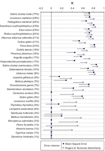
In order to summarize the differences between the conventional (MSE-based)

ANN model and the enhanced (dissimilarity-based) one, it is useful to compare

the K statistics species by species, as shown in Fig. 3.8.5. The small boxes show

the K values for the conventional model (solid boxes) and for the enhanced one

(white boxes), while the whisker on the left of each box indicates the lower end of

the confidence interval of the K statistics (the upper one is not relevant in this

case, so it was omitted). Obviously, the K statistics is not significantly different

from zero (at a probability level p=0.95) if the left whisker intersects the vertical

axis at K=0. The boxes on the vertical axis with no whisker on the left show those

cases in which the K statistics was not computed because the model always

pre-dicted the absence of the corresponding species. The species have been sorted

ac-cording to their frequency, shown in parentheses on the right of each species

name.

It is very easy to notice that there were no cases in which the conventional

training provided higher K values than the enhanced model, but the most striking

difference between the two models can be observed for the less frequent species.

In fact, the enhanced model allowed obtaining dramatic improvements in the

pre-dictive ability of the model and in several cases the K statistics for the enhanced

model was significant, while it was not significant or not even computable for the

conventional model.

In the case of the enhanced model only five species were associated with values

of the K statistics that were not significant, while twelve species were in that

situa-tion when the convensitua-tional model was used. It is interesting to notice that the

largest changes in K values were observed for species whose frequency ranged

from 3% to 9%. These species, that cannot be considered as truly rare species, are

certainly associated with particular physical, chemical and biotical conditions and

play a relevant role in defining the ecological characteristics of the fish

assem-blage.

Table 3.8.4 Enhanced ANN model: observed and predicted frequency by species

(sorted in descending order of observed frequency) and K statistics (significant

values are marked with an asterisk).

observed frequency

predicted

frequency K

Salmo (trutta) trutta 76.5% 74.6% 0.726 * Leuciscus cephalus 28.0% 24.6% 0.805 * Padogobius martensii 26.1% 22.0% 0.767 * Scardinius erythrophthalmus 25.0% 23.5% 0.836 * Esox lucius 24.6% 21.2% 0.754 * Rutilus erythrophthalmus 24.6% 21.6% 0.765 * Alburnus alburnus alborella 21.2% 19.7% 0.790 * Cottus gobio 20.8% 12.5% 0.640 * Tinca tinca 20.1% 17.4% 0.824 * Cobitis taenia 17.8% 15.2% 0.675 * Phoxinus phoxinus 17.8% 14.0% 0.615 * Anguilla anguilla 17.4% 13.3% 0.721 * Knipowitschia punctatissima 17.0% 13.6% 0.665 *

Salmo (trutta) marmoratus 10.2% 9.1% 0.876 * Sabanejewia larvata 9.8% 8.3% 0.794 * Ictalurus melas 9.5% 8.3% 0.829 * Lepomis gibbosus 8.7% 2.3% 0.375 * Barbus plebejus 7.2% 4.5% 0.603 * Chondrostoma genei 6.8% 4.5% 0.709 * Gasterosteus aculeatus 6.8% 3.8% 0.601 * Carassius auratus 6.4% 1.9% 0.415 * Gobio gobio 6.4% 4.5% 0.603 * Leuciscus souffia 4.9% 2.3% 0.476 * Thymallus thymallus 4.9% 1.5% 0.458 * Lampetra zanandreai 3.8% 1.5% 0.485 * Gambusia holbrooki 3.4% 0.4% 0.195 n.s. Barbus meridionalis 3.0% 1.5% 0.560 * Micropterus salmoides 3.0% 1.1% 0.490 * Perca fluviatilis 1.1% 0.4% 0.497 n.s. Abramis brama 0.8% 0.4% 0.394 n.s. Cyprinus carpio 0.8% 0.0% 0.000 n.s. Salvelinus fontinalis 0.8% 0.0% 0.000 n.s.

-0.2 0 0.2 0.4 0.6 0.8 1

Salmo (trutta) trutta (77%) Leuciscus cephalus (28%) Padogobius martensii (26%) Scardinius erythrophthalmus (25%) Esox lucius (25%) Rutilus erythrophthalmus (25%) Alburnus alburnus alborella (21%) Cottus gobio (21%) Tinca tinca (20%) Cobitis taenia (18%) Phoxinus phoxinus (18%) Anguilla anguilla (17%) Knipowitschia punctatissima (17%) Salmo (trutta) marmoratus (10%) Sabanejewia larvata (10%) Ictalurus melas (9%) Lepomis gibbosus (9%) Barbus plebejus (7%) Chondrostoma genei (7%) Gasterosteus aculeatus (7%) Carassius auratus (6%) Gobio gobio (6%) Leuciscus souffia (5%) Thymallus thymallus (5%) Lampetra zanandreai (4%) Gambusia holbrooki (3%) Barbus meridionalis (3%) Micropterus salmoides (3%) Perca fluviatilis (1%) Abramis brama (1%) Cyprinus carpio (1%) Salvelinus fontinalis (1%) K

Rogers & Tanimoto dissimilarity Mean Square Error Error criterion

{

Figure 3.8.5 A comparison of K statistics values for the conventional model,

us-ing Mean Square Error as the error criterion (black squares), and the enhanced

model, using Rogers and Tanimoto (1960) dissimilarity instead (white squares).

The line on the left of each square shows the lower limit of the confidence interval

of the K statistics. Therefore, when the line (or the symbol) intersects the vertical

axis at K=0 the K statistics is not significantly different from zero (p=0.95).

8.8 Conclusions

Predicting the species composition of fish assemblages on the basis of

environ-mental descriptors is a feasible task that can be carried out either by means of

conventional probabilistic models (e.g. Oberdorff et al., 2001) or by means of

ANNs (e.g. Aguilar Ibarra et al., 2003; Joy and Death, this volume; Olden and

Jackson, 2001). In particular, ANNs have been successfully used in these

applica-tions, as they allow exploiting heterogeneous sources of information in a very

ef-fective way (Scardi and Harding, 1999). Moreover, ANNs may be easily enhanced

and adapted to specific modeling tasks (Scardi, 2001), as they are entirely

empiri-cal tools.

Even though ANN are the most effective tools for modeling species

composi-tion (Olden and Jackson, 2002), they cannot solve the problems that are related to

the lack of relevant information. In fact, in many cases the only predictive

vari-ables that are easily available for the modeler are those that can be obtained from

cartographic records or direct observation. Other sources of information that

in-volve sampling and laboratory analyses are usually less abundant and therefore

play a secondary role. Moreover, species distribution data are also scarce, and

dis-tributed in space according to the local resources for monitoring activities rather

than on the basis of a suitable and consistent sampling design.Therefore,

predict-ing the species assemblage composition is not feasible without compromises. For

instance, accurate ANN models can be trained at a regional scale, or focusing on

species assemblages simpler than communities. Our application, dealing with fish

assemblages in northeastern Italian streams and rivers, belongs to this category

and is certainly an example of successful modeling that can be used in practical

applications. For instance, our model can be considered as a generator of expected

fish assemblages, i.e. of biotic reference conditions in the light of the EU Water

Framework Directive.

In particular, our model predicts the assemblage structure on the basis of

envi-ronmental descriptors that are mainly (but not exclusively) focused on the

geo-morphological characteristics and is based on data about the real assemblages, as

observed in a number of real sites. Therefore, the predicted assemblage is not just

the one that is supposed to be present at a theoretical pristine site, but a

compro-mise that represents the more likely biotic response given a number of existing

constraints, mainly related to the long term anthropogenic impacts on pristine

eco-systems (e.g. changes in land usage, introduction of exotic species, modification

of river banks, etc.). In regions where pristine conditions do not exist since several

centuries, this is probably the only meaningful way to define reference conditions.

The ANN models we presented are not only an achievement in applied

ecologi-cal research, as they also point out more general problems in species distribution

modeling and provide solutions for them.

The most general scientific issue that emerged from our work is that very rare

and very frequent species cannot be effectively modeled unless enough

informa-tion is available. This obviously does not happen in many real studies, in which

the only acceptable solution should be based on several species-specific sampling

designs, i.e. on multiple sampling designs tailored to fit the distribution of each

studied species.

Another relevant scientific issue that was highlighted by our work was the need

for adequate error measurements in ecological applications. In fact, conventional

criteria like MSE may fail when applied to data that are not strictly quantitative,

like species presence and absence data. These data are binary from a formal point

of view, but they cannot be treated just as sequences of 1s and 0s. Each species

contributes to the assemblage structure in a way that depends simultaneously on

its ecological characteristics and on the composition of the assemblage. Therefore,

some errors in predicting species composition might be more relevant than others.

For instance, in many upstream sites the only fish species is Salmo trutta trutta,

which is also very frequent as a member of much more complex assemblages in

other sites downstream. It is obvious that not predicting its presence in an

up-stream site would be a much more severe error than not predicting its presence

elsewhere.

Using a binary dissimilarity coefficient instead of MSE as the criterion for

measuring prediction errors allowed obtaining a significant enhancement of a

con-ventional ANN model. Even though the functioning of the error back-propagation

algorithm was not changed, the modified training procedure relied on the

minimi-zation of the mean dissimilarity as a criterion for stopping the learning phase, thus

allowing optimal generalization of the model. In other words, the enhanced

train-ing procedure did not change the way the ANN model learned, but it changed the

conditions for stopping its optimization.

In our application the Rogers and Tanimoto (1960) dissimilarity was used,

be-cause we were confident about the reliability of our absence data and bebe-cause we

wanted to stress differences rather than resemblances between assemblages. In

dif-ferent situations, however, other coefficients would prove more adequate. For

in-stance, if absence data are not completely reliable (e.g. because of net avoidance)

an asymmetric dissimilarity that only takes into account presence data, like the

one based on the Jaccard’s coefficient (Jaccard, 1900, 1901, 1908), could be more

appropriate.

The enhanced training procedure not only improved the overall accuracy of the

predictions about species composition, but it also significantly increased the

abil-ity of the model to correctly predict rare species, thus mitigating the effects of the

unbalanced availability of information about rare species that was previously

men-tioned.

In order to obtain further improvements of species composition models,

how-ever, changes in the modeling strategies should be coupled with the optimization

of the sampling strategies. In fact, modeling rare or ubiquitous species is only

fea-sible if adequate information is available, as the ratio between the number of

ab-sence and preab-sence records in training and validation data set should be as close to

one as possible, while the variability of the environmental descriptors within each

subset, i.e. within the presence or absence subsets, should be maximum.

There-fore, ad hoc sampling designs that significantly deviate from the usual monitoring

approaches are needed. This shortcoming is not specific to ANNs, as it obviously

affects any modelling technique.

The enhanced ANN model presented in this chapter was incorporated into the

software tool that was published as one of the deliverables of the PAEQANN

pro-ject and that can be found in the CD attached to this book. Therefore, the readers

will be able to experiment the model on their own, to check its results and

com-pare the predictions it provides with those of other models.

8.9 Appendix

Both the percentage of Correctly Classified Instances (CCI) and the K statistics

(Cohen, 1960; Fielding and Bell, 1997) are based on the confusion matrix, i.e. on

a 2 x 2 contingency table in which predicted presence and absence of a taxon are

compared with their observed counterpart. In particular, if each case is expressed

as a proportion p

, then the confusion matrix will be

Predicted

1

0

1 p

p

Observed

0 p

p

and the sum of its elements will be 1. The CCI percentage will then be computed

as

∑

The K statistic can be easily computed from the same confusion matrix. The

observed (P

) and expected (P

) proportion of agreement between observed and

predicted data are the basis for the K statistics computation:

1 o e e P P K P − = −

In particular, P

is closely related to CCI%, whereas P

depends on the number of

cases in all the elements of the confusion matrix:

2 1 o ii i P p = =

∑

∑ ∑ ∑

In order to test the significance of the deviation from zero of the K statistics, the

standard error s

has to be computed, because the ratio between K and s

is

dis-tributed as the standardized normal variate Z. The standard error s

can be

ob-tained as

where n is the number of cases considered in the confusion matrix and C can be

obtained as

2 2 2 2 2 1 1 ij 1 ji 1 ij 1 ji i j j j j C p p p p = = = = = ⎡ ⎛ ⎞⎤ = ⎢ ⋅ ⋅⎜ + ⎟⎥ ⎢ ⎝ ⎠⎥ ⎣ ⎦

∑ ∑ ∑

∑

∑

It is very important, however, to remember that the standard error s

is not

ex-actly the same as the one that is needed, for instance, to compute the two-sided

confidence interval for K.

Acknowledgements

This chapter has been supported by the EU 5th Framework Programme PAEQANN pro-ject [“Predicting Aquatic Ecosystem Quality using Artificial Neural Networks: impact of environmental characteristics on the structure of aquatic communities (algae, benthic and fish fauna)”, URL: http://aquaeco.ups-tlse.fr/], under contract EVK1-CT1999-00026.

References

Aguilar Ibarra A, Gevrey M, Park YS, Lim P, Lek S (2003) Modelling the factors that in-fluence fish guilds composition using a back-propagation network: assessment of met-rics for indices of biotic integrity. Ecol Model 160: 281-290

Aguilar Ibarra A (2004) Les peuplements de poissons comme outil pour la gestion de la qualité environnementale du réseau hydrographique de la Garonne. PhD Thesis, Ecole National Supérieur Agronomique de Toulouse, Institut National Polytechnique, Tou-louse, France.

Allan JD (1995) Stream Ecology. Structure and Function of Running Waters. Chapman & Hall, London.

Angelier E (2001) Ecologie des Eaux Courantes. Tec & Doc, Paris.

Angermeier PL, Schlosser IJ (1995) Conserving aquatic biodiversity: beyond species and populations. Am Fish Soc Symp 17: 402-414

Angermeier PL, Winston MR (1998) Local vs. regional influences on local diversity in stream fish communities of Virginia. Ecology 79: 911-927

Angermeier PL (1994) Does diversity include artificial diversity ? Cons. Biol. 8: 600-602 Angermeier PL, Schlosser IJ (1989) Species area relationships for stream fishes. Ecology

70: 1450-1462

Armand C, Bonnieux F, Changeux T (2002) Evaluation économique des plans de gestion piscicole. Bull. Fr. Pêche Piscic. 365/366: 565-578

Backiel T, Penczak T (1989) The fish and fisheries in the Vistula River and its tributary, the Pilica River. In: Dodge DP (ed) Proceedings of the International Large River Sympo-sium, Honey Harbour, Ontario, Canada. Can Spec Publ Fish Aquat Sci pp 488-503 Balon EK (1975) Reproductive guilds of fishes: a proposal and definition. J Fish Res Board

Can 32: 821-864

Balon EK, Coche AC (1975) Lake Kariba, a man made lake ecosystem in Central Africa. Monographiae biologicae, 24 Junk The Hague, The Niederlands

Balon EK (1990) Epigenesis of an epigeneticist: the development of some alternative con-cepts on the early ontogeny and evolution of fishes. Guelph Ichthyol Rev 1: 1-48 Balon EK, Crawford SS, Lelek A (1986) Fish communities of the upper Danube River

(Germany, Austria) prior to the new Rhein-Main-Donau connection. Environ Biol Fish 15: 243-271

Baran P, Lek S, Delacoste M, Belaud A (1996) Stochastic models that predict trouts popu-lation densities or biomass on microhabitat scale. Hydrobiologia 337: 1–9

Baran P, Dauba F, Delacoste M, Lascaux JM (1993a) Essais d’évaluation quantitative du potentiel halieutique d’une rivière à salmonidés à partir des données de l’habitat physi-que. In: Gascuel D, Durand JL, Fonteneau A (eds). Les recherches françaises en éva-luation quantitative et modélisation des ressources et des systèmes halieutiques. Pre-mier forum halieumétrique, IRD Editions, Paris, pp 15-38

Baran P, Delacoste M, Lascaux JM, Belaud A (1993b) Relations entre les caractéristiques de l’habitat et les populations de truites communes (Salmo trutta L.) de la vallée de la Neste d’Aure. Bull Fr Pêche Piscicol 331: 321-340

Baran P, Delacoste M, Dauba F, Lascaux JM, Belaud A, Lek S (1995a) Effects of reduced flow on brown trout (Salmo trutta L.) populations downstream dams in French Pyre-nees. Regul. Rivers: Res Manage 10: 347-361

Baran P, Delacoste M, Lascaux JM, Dauba F, Segura G (1995b) La compétition interspéci-fique entre la truite commune (Salmo trutta L.) et la truite arc-en-ciel (Oncorhynchus

mykiss Walbaum): influence sur les modèles d’habitat. Bull Fr Pêche Piscic 337-339:

283-290

Baran P, Delacoste M, Lascaux JM (1997) Variability of mesohabitat used by brown trout populations in the French Central Pyrenees. Trans Am Fish Soc 126 : 747-757 Baran P, Lek S, Delacoste M, Belaud A (1996) Stochastic models that predict trout

popula-tion density or biomass on a mesohabitat scale. Hydrobiologia 337: 1-9 Barinaga M (1996) A recipe for river recovery? Science 273: 1648-1650

Bath NV, McAvoy TJ (1992) Determining model structure for neural models by network stripping. Comput Chem Eng 115: 271-281

Belaud A, Baran P (1997) Influence et détermination des débits réservés en rivières à sal-monidés. C R Acad Agric Fr 83: 65-74

Belaud A, Bengen D, Lim P (1989a) Observations sur la faune de poissons de la moyenne Garonne. Rev Géog Pyrén Sud-Ouest 60: 625-634

Belaud A, Bengen D, Lim P (1990) Approche de la structure du peuplement ichthyologique de six bras morts de la Garonne. Ann Limnol 26: 81-90

Belaud A, Chaveroche P, Lim P, Sabaton C (1989b) Probability-of-use curves applied to brown trout (Salmo trutta fario L.) in rivers of southern France. Reg Riv Res Manage 3: 321-336

Belaud A, Dautrey R, Labat R, Lartigue JP, Lim P (1985) Observations sur le comporte-ment migratoire des aloses (Alosa alosa L.) dans le canal artificiel de l’usine de Gol-fech. Ann Limnol 21: 161-172

Belaud A, Labat R (1992) Etudes ichtyologiques préalables à la conception d’un ascenseur à poissons à Golfech (Garonne, France). Hydroécol Appl 4: 65-89

Bellariva JL, Belaud A (1998) Environmental factors influencing the passage of allice shad

Alosa alosa at the Golfech fish lift on the Garonne River, France. In: Jungwirth M,

Schmutz S, Weiss S (eds) Fish Migration and Fish Bypasses. Fishing News Books, Oxford pp 171-179

Belliard J, Boët P, Tales E (1997) Regional and longitudinal patterns of fish community structure in the Seine River basin, France. Envir Biol Fishes 50: 133-147

Benchaken M, Loftus K, Wattanadilokgul C, Nuttasarin J (1989) Development of improved fisheries management program at Ubolratana reservoir, Thailand. Canada North-East Project. D.O.F./C.I.D.A. 906/11415 53p. Mimeo.

Bendell BE, McNicol DK (1987) Cyprinid assemblages, and the physical and chemical characteristics of small northern Ontario lakes. Environ Biol Fish 19: 229-234

Bengen D, Belaud A, Lim P (1992) Structure et typologie ichtyenne de trois bras morts de la Garonne. Ann Limnol 28: 35-56

Berkman HE, Rabeni CF (1987) Effect of siltation on fish communities. Environ Biol Fish 50: 133-147

Bernacsek G (1997) Management of Reservoir Fisheries in the Mekong Basin Project. Publ. Mekong River Commission, Bangkok Thailand

Berrebi-dit-Thomas R, Belliard J, Boët P (1998) Caractéristiques des peuplements piscico-les sensibpiscico-les aux altérations du milieu dans piscico-les cours d’eau du bassin de la Seine. Bull Fr Pêche Piscic 348: 47-64

Boet P, Fuhs T (2000) Predicting presence of fish species in the Seine river basin using arti-ficial neuronal networks. In: Lek S, Gueguan JF (eds), Artiarti-ficial Neuronal Networks: application to ecology and evolution, Environmental Science, Springer-Verlag pp 187-201

Bonnieux F, Vermersch D (1993) Bénéfices et coûts de la protection de l’eau : application de l’approche contingente à la pêche sportive. Rev Econ Polit 103: 131-152

Boulton AJ (1999). An overview of river health assessment: philosophies, practice, prob-lems and prognosis. Freshwat Biol 41: 469-479

Box GEP, Jenkins GM (1970) Time series analysis, Forecasting and Control. Holden-Day, San Francisco, USA

Brasquet C, Bourges B, Le Cloirec P (1999) Quantitative structure-property relationship (QSPR) for the adsorption of organic compounds onto activated carbon cloth: com-parison between Multiple Linear Regression and Neural network. Environ science Technol 33:4226-4231

Breiman L, Friedman JH, Olshen RA, Stone CJ (1984) Classification and regression trees. Wadsworth, Inc. Belmon, Calif. USA

Brosse S, Giraudel JL, Lek S (2001) Utilisation of non-supervised neural networks and principal component analysis to study fish assemblages. Ecol Model 146: 159-166 Bruslé J, Quignard JP (2001) Biologie des poissons d’eau douce européens. Editions Tec &

Doc, Paris

Bryce SA, Omernik JM, Larsen DP (1999) Ecoregions: a geographic framework to guide risk characterization and ecosystem management. Environ Pract 1: 141-155

Cattaneo F, Lim P, Belaud A (1999) Approche de la structuration spatiale du peuplement piscicole de la zone de transition de la Garonne. Ichtyophys Acta 22: 61-74

CBAG (Comité de Bassin Adour Garonne) 1996a Cahier géographique: Garonne. Comité de Bassin Adour Garonne, Toulouse

Changeux T, Bonnieux F, Armand C (2001) Cost benefit analysis of fisheries management plans. Fish Manage Ecol 8: 425-434

Chessman BC, Growns IO, Plunket-Cole N (1999) Predicting diatom communities at genus level for the biological management of rivers. Fresh Biol 41: 317-331

Chon TS, Park YS, Park JH (2000) Determining temporal pattern of community dynamics by using unsupervised learning algorithms. Ecol Model 132: 151-166

Chon TS, Park YS, Moon KH, Cha EY (1996) Patternizing communities by using an artifi-cial neural network. Ecol Model 90:69-78

Cisnereos-Mata MA, Bret T, Jarre-Teichmann A (2000) Performance comparison between regression and neural network models for forecasting Pacific sardine (Sardinops

caeruleus) biomass. In: Lek S, Guegan JF (eds) Artificial neural networks : application

in ecological modelling and evolution. Springer-Verlag

Cleveland WS (1979) Robust locally- weighted regression and scattered plot smoothing. J Am Statist Soc 74: 829-836

Cohen J (1960) A coefficient of agreement of nominal scales. Educ Psychol Measur 20: 37-46

Copp GH (1992) An empirical model for predicting micro habitat of 0+ juvenile fishes in a lowland river catchment. Oecologia 91: 338-345

Cowx IG, Welcomme RL (1998) Rehabilitation of Rivers for Fish. FAO & Fishing News Books, Oxford

Crespin BV, Usseglio-Polatera P (2002) Traits of brown trout prey in relation to habitat characteristics and benthic invertebrate communities. J Fish Biol 60: 687-714

Crisp DT (2000) Trout and salmon: ecology, conservation and rehabilitation. Fishing News Books, Blackwell Science, Oxford

Crül RCM (1992) Models for estimating potential fish yields of African inland waters. FAO/ CIFA Occasional Paper Roma

Cuinat R (1971) Principaux caractéres démographiques observés dans 50 rivières à truites françaises. Influence de la pente et du calcium. Ann Hydrobiol 2: 187-167

Daget J, Le Guen JC (1975) Dynamique des populations exploitées de poissons . In: La-motte M, Bourlière F (eds) Dynamique des populations de Vertébrés Publ. Masson. Paris France

Dauba F, Lek S, Mastrorillo S, Copp GH (1997) Long-term recovery of macrobenthos and fish assemblages after water pollution abatement measures in the river petite Baïse (France). Arch. Environ. Contam Toxicol 33: 277-285

Davies NM, Norris RH, Thoms MC (2000) Prediction and assessment of local stream habi-tat features using large scale catchment characteristics. Fresh Biol 45: 343-369 De Iong HH, Van Zon JCJ (1993) Assessment of impact of introduction of exotic fish

spe-cies in north-east Thailand. Aquacul Fish Manag 24: 279-289

De Silva SS, Moreau J, Amarasinghe US, Chookajorn T, Guerrero R (1991) A comparative assessment of the fisheries in lacustrine inland waters in three Asian countries based on catch and effort data. Fish Res 11: 177-189

De’ath G, Fabricius KE (2002) Classification of regression trees: a powerful tool yet simple technique for ecological data analysis. Ecology 81:3178-3192

De’ath G (2002) Multivariate regression trees: a new technique for modeling species-environment relationships. Ecology 85: 1105-1107

Dean T, Richardson J (1997) Native fish survival during exposure to low levels of dis-solved oxygen. Water and Atmosphere, 5: 12-14

Décamps H, Naiman RJ (1989) L’écologie des fleuves. La Recherche 208: 310-319 Delacoste M, Baran P, Dauba F, Belaud A (1993) Etude du macrohabitat de reproduction

de la truite commune (Salmo trutta L.) dans une rivière pyrénéenne, la Neste du Lou-ron. Evaluation d’un potentiel de l’habitat physique de reproduction. Bull. Fr. Pêche Piscic. 331: 341-356

Dimopoulos I, Chronopoulos J, Chronopoulos-Sereli A, Lek S (1999) Neural network models to study relationships between lead concentration in grasses and permanent ur-ban descriptors in Athens city (Greece). Ecol Model 120: 157-165

Dimopoulos Y, Bourret P, Lek S (1995) Use of some sensitivity criteria for choosing net-works with good generalisation ability. Neural Process. Lett. 2: 1-4

Dupias G, Rey P (1985) Document pour un zonage des regions phyto-écologiques. Centre National de la Recherche Scientifique, Toulouse, France

Dynesius M, Nilsson C (1994) Fragmentation and flow regulation of river systems in the northern third of the world. Science 266: 753-762

Ehrman JM, Clair TA, Bouchard A (1996) Using neural networks to predict Ph changes in acidified Eastern Canadian Lakes. Artificial Intelligence Applications 10:1-8

Emmons E, Jennings MJ, Edwards C (1999) An alternative classification method for north-ern Wisconsin lakes. Can J Fish Aquatic Sc 56: 661-669

Etchanchu D, Probst JL (1988) Evolution of the chemical composition of the Garonne river during the period 1971-1984. Hydrol. Sci. J. 33: 243-256

European Parliament 2000 Directive 2000/60/EC of the European Praliament and of the Council establishing a framework for Community action in the field of water policy. O.J. L 327, 72p

Fausch KD, Lyons J, Karr JR, Angermeier PL (1990) Fish communities as indicators of en-vironmental degradation. American Fisheries Society Symposium 8: 123–144

Faush KD, Hawkes CL, Parsons MG (1988) Models that predict the standing crop of stream fish from habitat variables: 1950–85. Gen. Tech. Rep. PNW-GTR-213. U.S. Department of agriculture, Forest service, Pacific north reaserch station, Portland, OR, 52 pp

Fielding AH, Bell JF (1997) A review of methods for the assessment of prediction errors in conservation presence/absence models. Environmental Conservation 24: 38-49 Froese R, Pauly D (eds) (2003) FishBase. World Wide Web electronic publication.

www.fishbase.org.

Garrison GD (1991) Interpreting neural network connection weights. Artificial Intelligence Expertise 6: 47-51

Gauch HG (1982) Multivariate analysis in community ecology. Cambridge University Press, Cambridge

Geman S, Bienenstock E, Doursat R (1992) Neural networks and the bias/variance dilema. Neural Comput 4:1-58

Gevrey M, Dimopoulos I, Lek S (2003) Review and comparison of methods to study the contribution of variables in Artificial Neural Network models. Ecol Model 160:249-264

Giraudel JL, Lek S (2001) A comparison of self-organizing map algorithm and some con-ventional statistical methods for ecological community ordination. Ecol. Model 146: 329-339

Giraudel JL, Aurelle D, Berrebi P, Lek S (2000) Application of the self-organizing map-ping and fuzzy clustering microsatellite data: how to detect genetic structure in brown trout (Salmo trutta) populations. In: Lek S, Guegan JF (eds) Artificial Neural Net-works: Application to Ecology and Evolution, Environmental Science. Springer, Berlin pp. 187-201

Gorman OT, Karr JR (1978) Habitat structure and stream fish communities. Ecology 59: 507-515

Gouraud V, Baglignière JL, Baran P, Sabaton C, Lim P, Ombredane D (2001) Factors regu-lating brown trout populations in two french rivers: application of a dynamic popula-tion model. Regul Rivers Res Manage 17: 557-569

Gouraud V, Sabaton C, Baran P, Lim P (1999) Dynamics of a population of brown trout (Salmo trutta) and fluctuations in physical habitat conditions -experiments in a stream in the Pyrenees; first results. In: Cowx IG (ed) Management and Ecology of River Fisheries, Fishing News Books, Blackwell Publishing, London pp. 126-142

Gozlan RE, Mastrorillo S, Dauba F, Tourenq JN, Copp GH (1998) Multi-scale analysis of habitat use during late summer for 0+ fishes in the River Garonne (France). Aquat Sci 60: 99–117

Grossman G, Ratajczac RE, Crawford M, Freeman MC (1998) Assemblage organization in stream fishes: effects of environmental variation and interspecific interactions. Ecol Monographs 68: 395-420

Guegan JF, Lek S, Oberdorff T (1998) Energy availability and habitat heterogeneity predict global riverine fish diversity. Nature 391: 382-384

Györgyi G (1990) Inference of a rule by a neural network with thermal noise. Phys. Rev. Lett 64: 2957-2960

Harding JS, Benfield EF, Bolstad PV, Helfman GS, Jones EBD (1998) Stream biodiversity: the ghost of land use past. Proc Nat Acad Sci US 95: 14843-14847