1
ALMA MATER STUDIORUM
UNIVERSITA’ DI BOLOGNA
Scuola di Ingegneria e Architettura
Sede di Forlì
Corso di Laurea Magistrale in
INGEGNERIA AEROSPAZIALE
Classe LM20
TESI DI LAUREA
In
DINAMICA E CONTROLLO ORBITALE
Simulation of Bistatic Radar Experiments with Deep Space
missions
CANDIDATO
RELATORE
Leonardo Gualchieri
Prof. Paolo Tortora
Anno Accademico 2015/2016
Sessione II
3
Abstract
L’obiettivo del lavoro esposto nella seguente relazione di tesi ha riguardato lo studio e la simulazione di esperimenti di radar bistatico per missioni di esplorazione planeteria. In particolare, il lavoro si è concentrato sull’uso ed il miglioramento di un simulatore software già realizzato da un consorzio di aziende ed enti di ricerca nell’ambito di uno studio dell’Agenzia Spaziale Europea (European Space Agency – ESA) finanziato nel 2008, e svolto fra il 2009 e 2010. L’azienda spagnola GMV ha coordinato lo studio, al quale presero parte anche gruppi di ricerca dell’Università di Roma “Sapienza” e dell’Università di Bologna. Il lavoro svolto si è incentrato sulla determinazione della causa di alcune inconsistenze negli output relativi alla parte del simulatore, progettato in ambiente MATLAB, finalizzato alla stima delle caratteristiche della superficie di Titano, in particolare la costante dielettrica e la rugosità media della superficie, mediante un esperimento con radar bistatico in modalità downlink eseguito dalla sonda Cassini-Huygens in orbita intorno al Titano stesso.
Esperimenti con radar bistatico per lo studio di corpi celesti sono presenti nella storia dell’esplorazione spaziale fin dagli anni ’60, anche se ogni volta le apparecchiature utilizzate e le fasi di missione, durante le quali questi esperimenti erano effettuati, non sono state mai appositamente progettate per lo scopo. Da qui la necessità di progettare un simulatore per studiare varie possibili modalità di esperimenti con radar bistatico in diversi tipi di missione.
In una prima fase di approccio al simulatore, il lavoro si è incentrato sullo studio della documentazione in allegato al codice così da avere un’idea generale della sua struttura e funzionamento. È seguita poi una fase di studio dettagliato, determinando lo scopo di ogni linea di codice utilizzata, nonché la verifica in letteratura delle formule e dei modelli utilizzati per la determinazione di diversi parametri.
In una seconda fase il lavoro ha previsto l’intervento diretto sul codice con una serie di indagini volte a determinarne la coerenza e l’attendibilità dei risultati. Ogni indagine ha previsto una diminuzione delle ipotesi semplificative imposte al modello utilizzato in modo tale da identificare con maggiore sicurezza la parte del codice responsabile dell’inesattezza degli output del simulatore.
I risultati ottenuti hanno permesso la correzione di alcune parti del codice e la determinazione della principale fonte di errore sugli output, circoscrivendo l’oggetto di studio per future indagini mirate.
5
Abstract
The objective of this work shown in the following report thesis concerned the study and simulation of bistatic radar experiments for planetary exploration missions. In particular, the work focused on the use and improvement of a software simulator already implemented by a consortium of companies and research institutes as part of a study for the European Space Agency (European Space Agency - ESA) funded in 2008 , and carried out between 2009 and 2010. The Spanish company GMV led the study, together with research groups of the University of Rome "La Sapienza" and the University of Bologna.
The work done has been focused on the determination of the cause of certain inconsistencies in the outputs relating to the part of the simulator, designed in MATLAB environment, aimed at estimating the characteristics of the surface of Titan, in particular the dielectric constant and the average roughness of the surface, by means of a downlink mode bistatic radar experiment performed by the Cassini-Huygens probe in orbit around Titan.
Bistatic radar experiments for the study of celestial bodies are present in the history of space exploration since the '60s, even though every time the equipment used and the phases of the mission, during which these experiments were carried out, were never specifically designed for the purpose. From here the need to design a simulator for studying various possible ways of experiments with bistatic radar in different types of mission.
In a first phase of approach to the simulator, the work focused on the study of the documentation attached to the code in order to have a general idea of its structure and functioning. This was followed by a phase of detailed study, determining the purpose of each line of code used, as well as verification in the literature of the formulas and models used for the determination of different parameters.
The second phase of the work involved direct intervention on the code with a series of investigations to determine the consistency and reliability of the results. Each investigation has provided a decrease of simplifying assumptions imposed on the model used so as to identify with greater security the part of the code responsible for the incorrectness of the outputs of the simulator.
The results obtained have allowed the correction of some parts of the code and the determination of the main source of error on the output, circumscribing the object of study for future targeted investigations.
6
7
Index
1 Introduction:... 11
1.1 Structure of the document ... 12
2 Bistatic Radar ... 13
2.1 Bistatic radar coefficient ... 15
3 RC-SIM Simulator ... 16
3.1 General introduction ... 16
3.2 Technical requirements ... 16
3.3 Structure of the simulator ... 17
4 Input initial condition ... 19
5 Geometry ... 22
6 Observables ... 27
7 Retreival... 32
8 Output and performances... 33
9 Investigations on the simulator ... 36
9.1 Investigation 1 ... 36 9.1.1 Hypothesis ... 36 9.1.2 Development ... 36 9.1.3 Results ... 37 9.2 Investigation 2 ... 37 9.2.1 Hypothesis ... 37 9.2.2 Development ... 37 9.2.3 Results ... 38 9.3 Investigation 3 ... 38 9.3.1 Hypothesis ... 38 9.3.2 Development ... 38 9.3.3 Results ... 40 9.4 Investigation 4 ... 40 9.4.1 Hypothesis ... 41 9.4.2 Development ... 41 9.4.3 Results ... 41 9.5 Investigation 5 ... 44 9.5.1 Hypothesis ... 44 9.5.2 Development ... 44
8 9.5.3 Results ... 45 9.6 Investigation 6 ... 46 9.6.1 Hypothesis ... 46 9.6.2 Development ... 46 9.6.3 Results ... 47 9.7 Investigation 7 ... 47 9.7.1 Results ... 48 9.8 Investigation 8 ... 50 9.8.1 Hypothesis ... 50 9.8.2 Results ... 50 9.9 Investigation 9 ... 51 9.9.1 Hypothesis ... 51 9.9.2 Development ... 51 9.9.3 Results ... 51 10 Conclusions ... 54 11 Future developments ... 55 12 Bibliography ... 56
9 Table of Figures
Figure 1 RC-SIM simulator flow chart taken from the Final Report of the simulator ... 17
Figure 2 Titan’s reference map for the dielectric constant... 20
Figure 3Titan's reference map for the sms-slope ... 21
Figure 4 Flow chart for the Geometry block ... 22
Figure 5 the angles that define the environment of the reflection of the signal ... 24
Figure 6 Flow chart for the Observables part ... 27
Figure 7 Power Spectral dencity: each point is the power received by a single scatterer ... 29
Figure 8 Envelope of the maximum of the PSD ... 30
Figure 9 Dielectric constant: reference value (blue) and retrieved value (red) ... 34
Figure 10 Relative error of the retrieved dielectric constant ... 34
Figure 11 rms-slope: reference value (blue) and retrieved values (red) ... 35
Figure 12 Relative error of the rms-slope ... 35
Figure 13 Coef term varying with che number of scatterer ... 40
Figure 14 Upq term varying with the number of scatterer ... 40
Figure 15 Bistatic scattering coefficient determined with modulus of TRAN_to_SURF equal to the modulus of SURF_to_RECV. Radius othe orbit 1500 km in black, 100 to 1400 km in red, 3000 to 40000 km in blue ... 43
Figure 16 Bistatic scattering coefficient derived with the real modulus of SURF_to_RECV and varying the modulus of TRAN_to_SURF. radius of the orbit 1500 km in black, 100 to 1400 km in red) 3000 to 40000 km in blue ... 43
Figure 17 Bistatic scattering coefficient derived with the real modulus of TRAN_to_SURF varying the modulus of SURF_to_RECV. Modulus of GS_Tit equal to 1500 km in black, 100 to 1400 km in red, 3000 to 40000 km in blue. ... 44
Figure 18 Rms-slope: retrieved values (red) and refernce value (blue) with the new method to define the incident and reflective unit vectors ( height from surface 1500 km) .... 45
Figure 19 relative error of the rms-slope ... 46
Figure 20 relative error of the retrieved rms-slopebefore the modification of the determination method or the relative velocity vector ... 47
Figure 21 relative error of the retrieved rms-slope in the case of revolution of hte celestial bodies applied to the scenario ... 48
Figure 22 rms-slope: retrieved (red) and reference (blue), 100 km from the surface... 49
10
Figure 24 Bistatic scattering coefficient varying from a distance of 100km to 4000 km
from the surface ... 52 Figure 25 bistatic scattering coefficient dependant to the doppler frequency and varying from a distance of 100 km from the surface to 4000 km ... 53
11
1
Introduction:
In the history of space exploration the use of radio waves between Earth and the S/C was primarily intended for communication purposes and also as a method for orbit determination of the S/C itself. However, the electromagnetic waves sent from Earth were also used to study some characteristics of the surface of planets and moons (such as estimating their roughness and the material of the surface) that can only be investigated by means of radio waves able to cross the clouds in the atmosphere (monostatic radar).
In the 60’s the radio communication systems were used for the first time in bistatic radar experiments to overcome the intrinsic problems in the planetary observation with the monostatic radar from Earth, such as the large distances which limit the sensitivity to specific characteristics of the observed surface or the impossibility to observe areas of the surface far from the equator (due to geometrical issues).
During bistatic radar investigations the signal was occasionally used to infer information on the planets when geometry permitted an occultation, often during other atmosphere/ionosphere radio sounding experiments. Anyway, this was never accomplished with appropriate devices designed at this purpose.
In response to the ESA/ESTEC ITT Reference AO/1-5915/08/NL/AF, the GMV company built up a simulator applicable to bistatic radar problems providing the estimation of near surface dielectric constant and root-mean-square value of the surface slope for different missions on Titan. The software has been implemented in MATLAB environment.
The estimation of the root-mean-square value of the surface slope (rms-slope) provided by the simulator is affected by an error approximately of 100% respect to the reference used in the calculations.
The scope of this work is to analyse the code and detect the areas subjected by the errors. The results obtained in the investigations are summarized with respect to the type of investigation adopted. First of all the verification of the formulae, then the checking of
12
the consistency of the various parts of the code (the calculations, the scenario etc..) and finally identifying precisely the possible source.
1.1
Structure of the document
Chapter 2 explains the principals of operation and the results that is possible to obtain using the technic of the bistatic radar and the use of this technic in previous missions. Chapter 3 provides a general introduction of the structure (the parts in which the simulator is divided) and the hypothesis used to create the simulator.
Chapter 4 describes the initial conditions for the simulation.
Chapter 5 explains the calculation process to create the data that describe the environment under the geometrical point of view, describing the most important steps in the determination of all the data required for the next part of the code.
Chapter 6 as Chapter 5 describes the main steps during the calculation of the observables of the simulated signal during the transmission to Earth.
Chapter 7 as well describes the code used to determine the retrieval of the data of the signal simulated and to create the result of the simulator
Chapter 8.describes the performances of the simulat with the default inputs and the error present in the outputs.
Chapter 9 describes the actions and modifications undertaken on the simulator to study the properties and to debug the code. Starting with the simplifications imposed to avoid unnecessary source of error (as the ones normally provided by the environment) other than the one in the code, following with the actions to verify each part of the code and find the source of the error.
Chapter 10 summarizes the results obtained in the study and provides conclusions Chapter 11 describes future developments
13
2
Bistatic Radar
The principle of radar operation consists in the generation of an electromagnetic wave (from the transmitter) which propagates and produces an echo of the signal when encountering the target that is captured back by the receiver. Normally, talking about radar suggests what it is more properly called “monostatic radar” where the transmitter creating the signal is in the same location of the receiver. Conversely, in bistatic radar configuration the location of the source station and the receiving station are in different locations: in this way one of the leg of the signal propagation can be extremely shortened using for example a S/C orbiting around the target.
The signal that impacts on the target interacts with it following the optical reflection rules even if the interaction with the surface that creates refraction/dispersion effects has an important contribution.
The interaction of the radio wave with the surface can be seen in Figure 1 where it is possible to observe the case of perfect reflection when the hypothetically singular incident ray impacts the surface that is perfectly plane. In this condition the only effect that is produced follows the Snell’s first law (the angle between the incident ray and the normal to the surface is the same from the normal to the surface and the reflective direction). When the surface is not perfectly flat neither highly rough, the echo of the singular incident ray is characterized by a part where the signal follows the reflection direction (known as the coherent reflection) and a part that has a diffusive effect and scatters the signal in various directions (known as the incoherent reflection) due to refraction effects , in particular because the distance between the surface ridges and the
wavelength of the signal are comparable.
When the roughness increases considerably with respect to the wavelength, the refraction effects are prevalent and the echo is mainly characterized by the diffusion part.
It is important to notice that the roughness alone is not sufficient to predict the response of the echo since this is also dependent on the interaction between the wavelength of the signal and the distances between the ridges that create the roughness of the surface. In fact, a surface which is seen as rough when illuminated, could appear flat, or nearly
14
so, if hit by an electromagnetic wave with longer wavelength. A similar effect can be seen also with water waves, for example in proximity of breakwaters in a harbour: when the wavelength of sea waves is comparable to the distances between the breakwaters a refraction effect exists that creates a serial of circular waves on the other side of the breakwater. When instead the sea wave has a longer wavelength there is no refraction effect, the sea wave is entirely reflected back because the distance between the breakwaters is too small and the series of breakwaters is equivalent to a singular wall.
The use of telecommunication systems for bistatic investigations was exploited thanks to the frequency employed for the radio waves. in fact, their wavelength was of the order of centimeters/meters, the correct length to investigate the surface for possible landing sites and also for geophysical purposes.
Usually, missions comprising bistatic radar investigationsmake use of signals in the S-,X-,Ka- band, respectively at 2.5, 8.5 and 32 GHz .
These expriments can be performed via two different configurations: - uplink bistatic radar
- downlink bistatic radar
In the uplink mode the transmitter is located on Earth and the receiver is on board the S/C, while the downlink mode is the opposite.
uplink bistatic radar has the advantage of a larger power capability which means a higher SNR thus leading to a more precise reception of the signal (he transmission power of the ground station that can be greater than 1 MW). On the other hand, it is more difficult to aim precisely to the target and also to keep a sufficient directivity of the signal to impact a particular area of the surface.
The downlink mode instead, even if characterized by a lower power (normally in the order of 100 W), can interact with a more limited area and investigate at a better level of accuracy also regions that are almost impossible to be studied in the uplink mode due to geometrical configurations. Another disadvantage, other than the SNR received on Earth, is the necessity for the S/C to precisely address a specific area of the target so that
15
the reflected signal is correctly received on Earth, that means an accurate series of manuvers to properly orient the S/C.
Historically, in the majority of the cases where bistatic radar investigations were carried out, they were performed in downlink mode, since the S/Cs were not equipped with the receiver on board,
2.1
Bistatic radar coefficient
The bistatic radar is a particular kind of radar where the transmitting location and receiving location are different. The formula which describes the power received by the receiver is �� � �������������� �4���� ������� � ���������������� �4���� �������
This formula is due to the propagation of the signal. In fact the transmitting power can be imagined propagating in spherical wave, the transmitting gain correct this due to the directivity of the antenna. The spherical wave impacs on a surface distant Rtx from the source and is reflected as another spherical wave to the receiver distant Rrx from this surface. At the end the power per unit area calculated is multiplied for the antenna effective area (equal to ���� ) permits the evaluation of the received power. The ���� , called the radar cross section, is necessary to describe the modification of the signal due to the electromagnetic interaction with the surface. This radar cross section is
independent by the kind of incident electromagnetic wave and depends only on the geometry of the impact and the geometrical and geophysical characteristics of the surface. This parameter is misured in m2, in fact it is equivalent to an area that is not
related with the real surface of impact. It is an area proportional to the characteristics of reflectivity of the body. When the electromagnetic wave impacts on a body that is quite large as in this case, often is preferable to use the bistatic scattering coefficient instead of the radar cross section.
There are different models to determine bistatic radar coefficient, differing by the range of applicability. Normally the model used in the simulator is the Geometric Optic theory but recent improvements of the Physical optic theory even for the range of applicability of the Geometric Optic theory permits its application in the code.
16
3
RC-SIM Simulator
3.1
General introduction
The RC-SIM project as the subtitle suggests, “RC-SIM Radiocomm Signal: a “new” way of probing the surface of planets”, has the scope to determine and verify new methods of determining the characteristics of the surfaces of planets and moons using bistatic radar experiments in different kind of scenarios and missions.
There are three main scenarios around different celestial bodies: - Titan (scenario 1);
- Mars (scenario 2); - Moon (scenario 3);
Each one with different specifics and aims. The scenario under investigation of this work is the Scenario 1 which, in turn, is composed by four sub-scenarios:
- Scenario 1a = downlink experiment between S/C and Ground Station (GS) - Scenario 1b = downlink experiment between S/C and a Balloon in the Titan
atmosphere
- Scenario 1c = downlink experiment between S/C and GS - Scenario 1d = uplink experiment between S/C and GS; The sub-scenario of interest is the first one (1a)
An important assumption that has been made in the implementation of the simulator is that the speed of light is not considered in the propagation of the radio wave. The velocity of the signal is supposed to be infinite, that is the celestial bodies remain in the same position state they have when the signal departs, and during the entire propagation of the radio wave.
3.2
Technical requirements
The simulator was designed to operate on Windows XP 32-bit version, so that it is possible to use the libraries containing JPL calculations for the ephemerides of the planets and the principal moons of the Solar System. In order to operate the simulator on newer Windows operative systems (expecially the 64-bit ones) it is indeed necessary to provide a 32-bit version of MATLAB and also install aVisual C++ 2005 Redistributable x86 version (normally absent in 64-bit operative systems like Windows 7 or later). For this work Matlab 7.10.0 (R2010a) was used.
17
3.3
Structure of the simulator
The simulator functionality can be visualized in the flow-chart below:
Figure 1 RC-SIM simulator flow chart takenfrom the Final Report of the simulator
The entire mode of operation of the simulator is centered on the “Controller” block which coordinates all the routines and initializes the following parts using as inputs the results calculated in the previous ones.
At first, the Controller block starts the Input parameters function that creates a series of structure files in which all the values imported from scheduled data are summarized. The input parameters are imported in the Geometry function with other parameters and scheduled data, such as JPL ephemerides of the celestial bodies, and their rotational state. At the end of the block, all the calculations define the entire geometry of the environment. These data are saved and then imported in the Observables function that uses the relative positions of the S/C and the celestial bodies to determine the characteristics of the signal propagating from the S/C to the Ground Station (GS). In particular, it simulates the shape of the Power Spectral Density (PSD) of the signal for the left- and right- circular polarization .
18
All the relevant data acquired in the Observables function are then imported in the Retrieval function where the final data of the simulation together with the reference values are computed.
At the end of this procedure the Output function plots the data relevant for the simulation and saves all the data in .mat files (Matlab extension) that are divided in different folders depending on their type
In the following chapters the main blocks will be described in detail: - Initial conditions
- Geometry - Osservables - Retrieval
19
4
Input initial condition
In the first part of the code the initial conditions needed in the simulator are acquired. Four different structure files are created:
- scenario1_param
- simulation_param
- radiosystem_param
- signal_propag_param
The scenario1_param file contains all the initial parameters concerning the environment, for example spacecraft orbit data (inclination, RAAN, radius, initial state vector, initial velocity vector, etc…), Titan surface map (for the dielectric constant and the rms-slope), number of point in which the footprint of the antenna is divided.
The simulation_param file contains the input parameters involving the specifications for the simulation such as the duration of the simulation, the timestep used during the orbit propagation of the S/C, the epoch expressed in Julian date (J2000), the geodetic coordinates of the Ground Station and the possible source of error in the location of the orbiter around Titan.
The Radiosystem_param file defines all the parameters involving the telecommunication systems as the dimensions, the elevation angle and the azimuth angle of the G/S antenna and the Orbiter antenna as well as the frequency (GHz) and power (dBm) of the transmitted signal.
The Signal_propag_param file contains the physical constants related to the electromagnetic waves (such as the speed of light, the vacuum permittivity and permeability and all the sources of error that can influence the signal).
For the present research all the errors are set to zero since the initial step to be perfomed for detecting the error affecting the code is to identify possible mistakes in ideal conditions. In particular the following sources of error are temporarily discarded:
- Orbit perturbations parameters: o Non spherical gravity field o Solar radiation
o Third bodies
- Error model for orbiter location uncertainty - Error model for station location uncertainty - Error model for plasma delay
- Error model for uncalibrated ground station delay - Error model for ground antenna mechanical noise - Error model for tropospheric noise
20
The most relevant parameters during the investigation were: - Height at pericenter from Titan surface (default 1500 km ) - Height at apocenter from Titan surface (default 1500 km ) - Orbit inclination (default 82°)
- Orbit right ascension of the ascending node [RAAN] (default 0°) - Elevation angle of the antenna on the S/C (default 5°)
- Azimuth angle of the antenna on the S/C (default 5°)
- Number of points which divide the latitude of the footprint of the antenna (default 20)
- Number of points which divide the longitude of the footprint of the antenna (default 20)
- Time resolution (default 60 s) - Titan map (used as reference)
To establish a reference value for the simulator, it is used a grid of values for the dielectric constant and for the rms-slope, both varying with latitude and longitude (1° resolution) so that all the surface of Titan is covered.
The default map used is called Titan_map_er23_slope101.mat that contains the grid of dielectric constant values ranging from 2 to 3. The lesser value represents liquid areas :
Figure 2 Titan’s reference map for the dielectric constant
The values distribution for the rms-slope of the surface in the grid is in part dependant to the distribution of the dielectric constant values. It is necessary that every liquid area in the dielectric reference map is a flat area and so the value of the rms-slope has to be the minimum available. Obviously there can be flat areas even in solid areas, in fact
21
there are areas with a low value of the rms-slope in other regions of the map, in particular in the equatorial region.
Figure 3Titan's reference map for the sms-slope
22
5
Geometry
23
This flow chart represents the passages in which the code for the Geometry function can be divided. Every block corresponds to a set of instructions that will be explained in detail below:
The four upper block represents the four structure files created by the input block and imported here.
1. Initial condition = together with the previous imported data, to perform the code it is necessary to add other information about physical characteristics of the planets and moons of interest in the calculation (radius, gravitational constant of the body etc…) which refers to the JPL ephemerides de118 and de200.
2. Orbit propagation = in this block the orbit of the S/C is determined. At first the initial condition for the propagation are calculated turning the keplerian elements, that describe the orbit and the position of the S/C, in a state vector with cartesian coordinates expressed in the MEE2000 reference frame. After this the orbit propagation is performed by an explicit embedded Runge-Kutta integrator which integrates a system of ordinary differential equations using 8-7 th order Dorman and Prince formulas. This integrator requires 13 evaluations; the higher order of the schema (8) is used to optimize the solution, while the lower order(7) is used to perform stepsize control. After that the propagation is completed, the results are elaborated to determine the S/C position at each time of integration, the time vector as well as the vector that describes the angular velocity of Titan around its rotational axis.
3. Propagation of Celestial bodies = in this block the ephemerides of each celestial body of interest is calculated using the JPL ephemerides. In particular the position vector for Titan and Earth respect to the Sun is evluated. In addition all the vectors which describe the relative positions between S/C, Earth and Titan are also computed.
4. Ground station parameters and visibility = Starting from the geodetic coordinates of the chosen GS, the code calculates the vector describing the position of the GS respect to the center of the planet expressed in the MEE2000 reference frame. To determine this vector the ECEF2ECI function is used; it rotates the input coordinates from ECEF (Earth Centered Earth Fixed ) reference frame to ECI (Earth Centered Inertial ) coordinated system. Moreover an analysis of the possibility of an eclipse of the S/C due to Titan, Saturn and Sun is performed; filtering the data to erase all this cases.
5. Center of the Scene coordinates and rotational matrix = this part of the code refers to the acquisition of the data about the position of the center of the footprint of the antenna. As visible in Errore. L'origine riferimento non è stata trovata. this point is also the specular point which permits the transmitted signal to propagate directly toward Earth. First of all the GTP angle (Ground-Titan_Probe angle) is computed using the invers function of the law of cosines. Considering the half of the GTP angle, using the sine law is possible to compute the angle α and then the angle β = α+GTP/2. This is the initial point for an optimization of the angle so that the final
24
value of β, now called Reflection angle, and γ respect the request of specularity for the incident and reflective direction respect to the normal to the surface.
Now is possible to compute the coordinates of the specular point, also called Center of the Scene. Primarily it is necessary to calculate a rotational matrix that refers to a local reference frame centered on Titan where the x-z plane contains the vector of the S/C and the vector that is directed from Earth to Titan. The y-axis complete the right-handed coordinated system.
Figure 5 the angles that define the environment of the reflection of the signal
The following passage is about rotating the Center of the Scene vector that can be computed as below using the rotational matrix previously calculated:
�� � �������cos � , ������sin � , 0�
so that the specular point is now computed for each time of propagation of the S/C.
It is also important to create an other rotational matrix able to rotate vectors from MEE2000 to the local reference frame centered on the specular point and called CS_rf. To do so it is necessary to create for each time of the simulation a local reference frame, using the Gram-Schmidt algorithm, takeing the vector from the center of Titan to the specular point (CS_Tit) and the vector from the specular point to the S/C (TRAN_to_SURF), both expressed in MEE2000.
6. Velocity vectors = this part of the code computes the velocity vector of the Center of the Scene, transmitter (S/C) and receiver (GS), all of them respect to the center of Titan. The function used rotates the position vectors from MEE2000 to the rotational celestial reference frame (RCBF) centered on Titan and then the time derivative is computed (difference of the coordinates of two consecutive vectors divided by the time step od the propagation). After this the computed velocity vector is rotated back to MEE2000 and then to CS_rf (using the rotational matrix calculated before). Moreover the transmitter and the receiver antenna directions are computed.
25
7. AdqArea:scatterers determination = this is a function called by the code to compute the coordinates of the scatterers which are distributed on the footprint of the antenna. These scatterers are the points that are meant to reflect the incoming signal toward Earth and where the signal interacts with the surface modifying the power specral dencity of the signal itself.
7.1. Direction of intersection illuminated area by radar = in this part of the code four unit-vectors are computed; they are used to determine the planes that define the intersection of the area illuminated by the radar using the elevation angle and the azimuth angle of the antenna. The elaboration of these unit vectors permits to obtain the four directions of the intersection of the four planes.
7.2. Rotational matrix transmitter = in this block of code the rotational matrix for the azimuth and elevation directions is computed. With the Gram-Schmidt algorithm, it is possible to compute a right-handed coordinated system using the previously calculated direction of the antenna and the direction of the velocity of the S/C, where the y-axis is the direction of the antenna itself. In this way it is possible to rotate the four intersection directions with the surface, computed in the previous block, to the rotational celestial body frame.
7.3. Grid points coordinates and vectors = with the intersection direction of the illuminated area with the surface, the surface intersection point,at the corners of the footprint area, can also be expressed in RCBF so that it is possible to evaluate the longitude and the latitude of each point.
7.4. Grid contruction = this part of the code determines the length and the width of the footprint area and creates a series of points linearly distributed dividing the side of the footprint area with a number of points chosen in input. After this the grid points in the planetodetic form are rotated back in the Cartesian form so that it is possible to calculate the position vectors of the scatterers respect to the center of Titan.
8. Vectors relative to scatterers = in this section the vectors of the scatterers are rotated from RCBF to MEE2000 and then they are used to evaluate all the vectors between the scatterers and the other parts that are in the environment like the S/C and the GS. 9. Incidential and reflective unit vectors for scatterers = in this part are computed the incident and reflective directions of the signal for every scatterer expressed in CS_rf. This means that it is sufficient to rotate, from MEE2000 to CS_rf , the unit vectors derived from the vectors TRAN_to_SCATT ( from the S/C to scatterers) for the incident directions and SCATT_to_GS (from scatterers to the GS) for the reflective ones. This unit vectors represent the direction of propagation of the signal..
10.Incidential and reflective unit vectors for the horizontal and vertical polarization = the following calculations need the incident and reflective directions of the horizontal and vertical polarization which form a right-handed coordinated system with the direction of propagation of the signal. At first are evaluated the unit vectors of the normal to the surface for every scatterer; they can be computed rotating to CS_rf the unit vector derived from SCATT_mee2000_tit (the vector from the center of Titan to scatterers). The horizontal polarization unit vectors are evaluated computing the cross product of the directions of the normal to the surface and the
26
directions of propagation of the signal. The vertical polarization unit vectors as well are evaluated with a cross product of the directions of propagation of the signal and the horizontal polarization unit vectors.
11.Relative velocities = to evaluate the Doppler frequency for each scatterer it is necessary to compute the relatve velocity for each scatterer respect to the S/C and the GS. These relative velocities have to be rotated to CS_rf.
27
6
Observables
28
This flow chart explains the mode of operation of the code which determines the observables used in the following calculations. As in the previous chapter, the code is divided in blocks that describe the main passages in the calculations and explained in detail below:
1. Initial conditions = first of all the reference map for the dielectric constant and the rms-slope are imported together with all the other parameters concerning the characteristics of the surface of Titan. Then all the transmitting and receiving antenna gains are acquired from the input structure files. Because of the resolution of the reference maps, an interpolation of the data is needed to find the exact value of the reference at the longitude and latitude which identify the scatterers during the entire simulation.
2. Doppler frequency computation = because of the motion of the S/C, Titan and Earth, a spectral broadening due to a Doppler frequency effect is unavoidable. To determine the entity of this frequency shift, it is necessary to determine the relative velocity between the scatterers and the other objects in motion, in particular the component of the velocity in the direction of the local normal to the surface. To do so it is sufficient to compute the scalar product of the relative velocity vector and the unit vectors of the normal to the surface of each scatterer. Using the simplified formula to determine the Doppler shift, it is sufficient dividing the previously computed relative velocity component with the wavelength of the signal. This calculation is performed for the transmitted signal and for the reflected signal separately but then the results are summed to find the actual Doppler frequency received by the GS.
3. Fresnel reflection coefficients = the Fresnel reflection coefficients describe the interaction of an electromagnetic wave that moves from a medium of a specific refractive index into another medium with a different refractive index. In particular they describe what fraction of the electromagnetic wave is reflected and what fraction is refracted. They depend on the polarization of the wave (horizontal, vertical or circular).
4. Scattering coefficient factor U = mn terms are valid only under Geometric Optics (GO) approximation, assuming a rough surface scattering bistatic problem and using the Forward Scattering Alignment (FSA) coordinate system. Umn terms are based on different scalar product combinations of unit vectors of the horizontal and vertical polarization corresponding to observed and incident waves.
29
5. Bistatic scattering coefficient = this block performs the final calculations to derive the bistatic scattering coefficient which require all the previous coefficients computed.
6. PSD calculation (radar equation) = the power spectral dencity of the received signal is computed evaluating the radar equation.
�� � ����������� ��� �4���� ������� � ������� ��� ������ �4���� �������
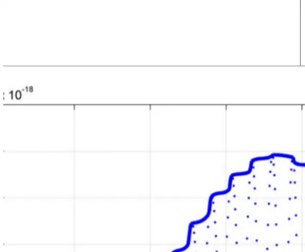
7. Post-processing = the PSD computed in the previous block is not suitable to be used in the following calculation. Some other computation is needed.
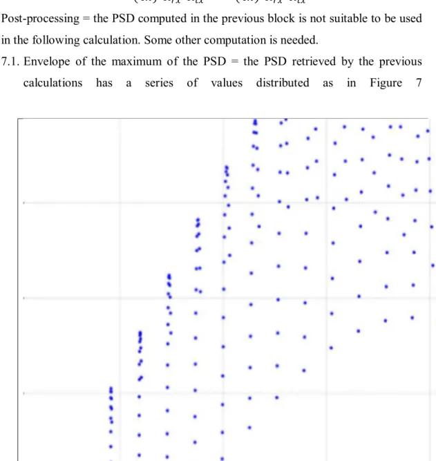
7.1. Envelope of the maximum of the PSD = the PSD retrieved by the previous calculations has a series of values distributed as in Figure 7
Figure 7 Power Spectral dencity: each point is the power received by a single scatterer
The evaluation of the envelope of the maximum values of the curve is required. The resulting curve shown in Figure 8.
30
Figure 8 Envelope of the maximum of the PSD
7.2. First estimation of the fitting Gaussian curve = this block computes the evaluation of the mean value of the Doppler frequencies weighted by the value of the power signal. Also the standard deviation is evaluated taking two point of the normalized envelope curve with a value higher than 0.8. The standard deviation of the curve is computed with the inverse function of the normal Gaussian curve in which the two chosen points are evaluated.
7.3. Non linear fit of a Gaussian curve to the data = The mean value of the Doppler frequencies and the standard deviation computed before are the initial guess for an optimization of the fitting Gaussian curve.
7.4. PSD Gaussian post-processed = in this block the parameters computed in the previous block are used to evaluate the final Gaussian curve fitting the PSD. 8. Weighted reference observables = it is necessary to evaluate a reference to compare
the final results. For this reason the latitude and longitude of the specular point and the other scatterers are used to evaluate the rms-slope and the dielectric constant for each scatterer. At the end of the process only a mean value for the entire footprint is
31
required, so a weighted mean is computed using the inverse of the distance of the scatterers from the specular point as weight.
32
7
Retreival
This part of the code is the crucial part that determines the final result of the simulation. Importing from the other parts of the code all the results acquired during the simulation, the code computes the modulus of the velocity of the Center of the Scene and the reflection angle previously calculated. For each instant of simulation considered, the code compares the LCP and the RCP simulated signal and chooses the greater value of them. Then the frequency of the signal is computed adding the mean frequency of the Doppler frequencies for each instant of simulation to the carrier of the original signal. Then the code computes the 3dB bandwidth value (BW3dB) equal to the standard deviation of the Gaussian curve fitting the PSD multiplied by 2.
At this point it evaluates the wavelength using the frequency previously computed and determines the rms-slope value for each instat of simulation using the formula below:
�������� � ��3�� �
33
8
Output and performances
The default set of input keplerian parameters for the simulation are:
Pericenter height (from surface) 1500 km
Apocenterheight (from surface) 1500 km
RAAN 5°
Inclination 82°
Argument of Periapsis 0°
True anomaly 0°
Number of scatterer in the footprint of the antenna 400 (20x20)
Azimuth angle of the Orbiter antenna 5°
Elevation angle of the Orbiter antenna 5°
Epoch (Julian day J2000) 5640
These are the main parameters that define almost the entire scenatio, in particular under the geometrical point of view. At the end of the routine the following results are shown: In Figure 9 the retrieved value of the dielectric constant is compared with the reference velue, while in Figure 10 the relative error is shown.. It is possible to notice that the retrieval of the dielectric constant has an high accuracy with most of the values of the relative error under the 0.5%.
Figure 11 and Figure 12 instead are about the retrieval value of the rms-slope, in particular in Figure 11 the retrieved rms-slope is compared to the reference value while Figure 12 shows the relative error.
It is important to notice how the relative error of the retrieved rms-slope is almost equat to 100% for most of the cases. The research of the source of this error in the rms-slope is exactly the purpose of this work.
34
Figure 9 Dielectric constant: reference value (blue) and retrieved value (red)
35
Figure 11 rms-slope: reference value (blue) and retrieved values (red)
36
9
Investigations on the simulator
After reading the documentation provided by GMV on the mode of operation of the simulator, about the performances of every part of the code, a verification of all the formulas used during the calculations was started. Then the code was studied accurately to achieve a deep knowledge of the purpose of every single line of code and evaluate the consistency of the scenario.
For these reasons a series of investigations were set to evaluate the features of the simulator varying with the complexity of the scenario, in particular varying the motion of the celestial bodies.
9.1
Investigation 1
9.1.1
Hypothesis
To study the consistency of every major task a first investigation is started in which all the celestial bodies and the S/C are stopped, so it is possible to study the simulator in a qualitative way.
9.1.2
Development
With the initial hypothesis and the fact that the speed of the signal is supposed infinite, the signal does not have a Doppler effect which means that with no spectral broadening it is impossible to determine the dielectic constant and the rms_slope. The only possible investigation is about the PSD of the signal that arrives to Earth, respect to the PSD at the starting point.
For this reason before starting this simulation it is necessary to provide some modification to the code to permit its operation. In the Geometry part it is necessary to create the velocity vector of the S/C, even if it is supposed to be fixed in a single position, because it is necessary for the creation of reference frames used to establish the orientation and the positions of the scatterers . It would be possible to avoid this counterintuitive method rewriting all this part of the code to be consistent with the hypothesis, but it surely time consuming, expecially for a qualitative investigation. Anyway the hypothesis are met because even if the velocity of the S/C is calculated, it
37
is not used in the determination of the relative velocity necessary to evaluate the Doppler frequency, in fact this parameter is imposed equal to zero.
9.1.3
Results
The resulting PSD provided by the Observables part of the code, as it can be imagined, is characterized by a single line in correspondence with the initial frequency at the start of the propagation by the S/C. This is in accordance with the theory and so there is consistency in the qualitative responce of the code.
It is important to notice that in this first case the number of scatterers used in the simulation was not modified, so the single resulting line in the PSD at the end of the calculations was indeed provided by a series of results with different value of power but with the same single frequency value, that can be expected with this initial hypothesis.
9.2
Investigation 2
A second investigation similar to the previous one was done to evaluate the entity of the Doppler effect in the simulation.
9.2.1
Hypothesis
This time the S/C is the only body in motion in the entire environment. The hypothesis for this investigation are that a single ray is sent by the S/C.
9.2.2
Development
To simulate this case is necessary to reduce the number of scatterers involved in the calculation from the default value of 400 to 1. In this way the simulation has in output only one value for the PSD, instead of a spectral broadening due to the presence of various scatterers with different relative velocities and so different contribution to the Doppler effect.
To implement this modifications in the code it is necessary to modify the number of point in which the footprint is divided. It is not possible to set directly only one point as a scatterer because an important parameter in the determination of the bistatic scattering coefficient, and so of the PSD, is the area of the scatterer that normally is evaluated dividing the area of the footprint for the number of scatterers. With only one point obviously it is impossible to determine the footprint area, so the minimum number of points is 4, necessary to create the footprint of the antenna with that particular elevation angle and azimuth angle as in input. After the computation of the value of the area for each scatterer, it is now possible to modify the code so that a single point is considered.
38
This single point can be found as the center of the footprint, calculating the mean value for the latitude and longitude of this four points.
9.2.3
Results
At the end of the calculations, in consistency with the modifications applied, the PSD of the simulation of the received signal is a single value and the frequency corresponding to this has a Doppler shift respect to the frequency at the start of the propagation.
The results provided by this investigation confirm the consistency of the model and also the furmula for the evaluation of the Doppler frequency.
9.3
Investigation 3
The previous investigations show that there is consistency in the determination of the geometry of the environment and the determination of the Doppler shift. The information about the power level received by the GS instead is not verified. The only characteristic that can be evaluated and that is consistent with the scenario is that the power level at the Earth is smaller than of the one at the start of the propagation.
9.3.1
Hypothesis
Looking ar the retrieval formula for the rms-slope , the factor that is more probably the cause of the error in the determination of this output parameter, is the standard deviation of the PSD. This value has a direct dependence with the spectral broadening and the level of power of each scatterer, in particular for those included in the envelopment of the maximum values. Due to the insurance of consistency of the Doppler frequencies computation by the previous investigations, the most probable source of error is due to the values of power for each scatterer. This parameter is in direct dependence with the bistatic scattering coefficient that determines the shape of the PSD.
Now it is important to determine what factor is responsible of the error in the determination of the bistatic scattering coefficient.
Since for the evaluation of the dielectric constant it is also used the PSD and since its evaluation is very accurate, with a mean relative error around 0.4%, it is possible to use these informations to determine the cause of the error.
9.3.2
Development
Since the dielectric constant is dependant to the ratio of the integral of the PSD for the left circular polarization and the right circular polarization, the formula of the Power received in the two polarizations, simplifying the common terms independent from the scatterers, can be expressed as below:
�� � � �∑ �� �� ∑ ���� � � � �∑ ����/�� ∑ ����/� �� � � � ∑ ���� ���/�� ∑ ���� ���/���
39 ���� � 8���|�1|���
����������� �
����������
�����������
The valoe of Rq is not constant because it represents the sum of the distances of the S/C
from the scatterer and the distance of the scatterer from the GS, for each scatterer considered. Indeed the values of Rq have a small variability, so in first approximation
these values can be approximated as constant so the expression of the dielectric constant is: �� ≅ � �∑ ���� ��� ∑ ���� ���� � � � �∑ ���� ��� ∑ ���� � �∑ ���� ��� ∑ ���� � � � � ��������� ��� ������
Where ������ represents the mean of ��� �� weighted by coef.
Looking at the shape of the coef term and ���, respectively in Figure 13 and Figure 14, due to their simmetry, the weighted mean is almost equal to the arithmetic mean, which means that
��_��������� ≅ � �∑ ����
∑ ����� ≅ � � ∑ ��� ∑ ����
40
Figure 13 Coef term varying with che number of scatterer
Figure 14 Upq term varying with the number of scatterer
9.3.3
Results
This means that the term that contributes to create the error in the rms-slope retrieved is located in the terms that are in coef because the information that is required to determine the exact retrieval of the dielectric constan is contained in the Upq term.
The coef term is dependant by various terms and those that can contribute in the onset of the error are especially qx,qy and qz that are terms dependant to the incident and reflective unit vectors for each scatterer.
9.4
Investigation 4
The results from the previous investigation lead to the discover of the most probable source of error for the retrieval of the rms-slope which is the interaction of the incident and reflective unit vectors of the scatterers within the retrieval formula for the rms-slope. For this reason the purpose of the following investigation is to determine the
41
dependence of the outcome of the bistatic scattering coefficient depending on the variation of these unit vectors.
9.4.1
Hypothesis
The method to determine the unit vectors normally consists in using the vector that define the position of the S/C and the vector of the position of the scatterers, both respect to Titan, to determine the difference vector and finally rotate them from MEE2000 to CS_rf and divide them for the modulus to create the unit vector. To study the properties of these unit vectors a new method to define them is provided
9.4.2
Development
Due to the interest in the response of the bistatic scattering coefficient formula from the variation of the direction of this unit vector, it would be sufficient to simulate the scenario with a variation of the modulus of the radius of the S/C orbit. To permit a right comparison of the results it is important that the local conditions are the same, expecially the elevation angle of the S/C in the local reference frame. For this reason the determination of these unit vectors in modified as follows:
It is calculated the difference vector of the scatterers and the CS vector (that corresponds to the specular point and the center of the footprint area) and then it is added the vector TRAN_to_SURF (that identify the distance from the S/C and the specular point). This method leads to an equivalent result of the previous one except for the fact that if the modulus of TRAN_to_SURF is changed, before the sum with the other vectors, it lead to a new set of unit vectors. To respect the consistency of the scenario, it is necessary that the velocity vector of the S/C is that of a circular orbit. For this reason for each value of the moduls of TRAN_to_SURF considered, it is calculated the modulus of the radius of the S/C orbit (adding the vector of the position of the specular point with TRAN_to_SURF) so that it is possible to evaluate the modulus of the S/C velocity for a circular orbit and multiply it for the appropriate unit vector of the S/C velocity. Moreover also the SURF_to_RECV vector (from scatterers to GS) modulus is modified to be fully aware of the dependency of the results from the characteristics of the unit vectors. Due to the peculiar characteristics of this investigation, a script separated from the actual simulator was written to avoid too many modification of the original code. The essential parts of the code were copied from the simulator and purposely adapted to the scope.
9.4.3
Results
In the following figures it can be seen the result of this investigation.
In Figure 15 the curves represent the bistatic scattering coefficient values varying with the modulus of TRAN_to_SURF and SURF_to_RECV; in x-axis the number of the scatterer in the grid. This is the case where the modulus of TRAN_to_SURF and
SURF_to_RECV is set to be equal so that the modulus of the radius of the orbit is equal to 1500 km (black curve). the red curves represent the cases for the modulus of the
42
radius that goes from 100 km to 1400 km, while the blue curves are from 3000 km to 40000 km.
In Figure 16 the modulus that varies is the one of TRAN_to_SURF while
SURF_to_RECV is equal to the real value. The radius of the orbit goes from 100 to 1400 km for the red curves, is equal to 1500 km for the black curve and goes from 3000 to 40000 km for the blue curves.
In Figure 17 what varies is the norm of SURF_to_RECV while TRAN_to_SURF remains at the original value. As in the previous figures the black lcurve represents the bistatic scattering coefficient derived by the algorithm with a norm of GS_Tit (from the center of Titan to the GS) equal to 1500 km, 100 to 1400 km for the red curves and 3000 to 40000 km for the blue ones.
As default result the simulator refers to the case represented by the black curve in Figure 16.
In first approximation it is possible to guess some feature about the standard deviation of the Gaussian curve that fits the PSD due to the fact that it is mainly the bistatic scattering coefficient that provide the shape of the resulting Gaussian curve and so also the standard deviation value. Indeed it can be noticed that the default case at 1500 km (the black curve in Figure 16) brings to a larger value of the standard deviation respect to the case at 1500 km in Figure 15, assuming that in both cases the S/C orbit is circular and so both cases have the same span of Doppler frequencies. It is important to notice that a comparison between two curves in the same figure does not bring for sure to an exact guess due to the fact that each curve has a different spectral broadening because of the different value of the velocity of the S/C.
43
Figure 15 Bistatic scattering coefficient determined with modulus of TRAN_to_SURF equal to the modulus of SURF_to_RECV. Radius othe orbit 1500 km in black, 100 to 1400 km in red, 3000 to 40000 km in blue
Figure 16 Bistatic scattering coefficient derived with the real modulus of SURF_to_RECV and varying the modulus of TRAN_to_SURF. radius of the orbit 1500 km in black, 100 to 1400 km in red) 3000 to 40000 km in
44
Figure 17 Bistatic scattering coefficient derived with the real modulus of TRAN_to_SURF varying the modulus of SURF_to_RECV. Modulus of GS_Tit equal to 1500 km in black, 100 to 1400 km in red, 3000 to
40000 km in blue.
9.5
Investigation 5
In this investigation the previous results for the bistatic scattering coefficient are implemented in the simulator to determine in the real scenario the contribution of the variability of the unit vectors evaluated with the method explained before.
9.5.1
Hypothesis
In this scenario the S/C is the only body in motion while the celestial bodies are stopped both in revolution and in rotation. The code that provided the results shown in Figure 15 and Figure 16 is implemented in the main code of the simulator. Various simulations are performed, each time changing the value of the norm of TRAN_to_SURF. This
procedure permits to study the importance of the distribution of the unit vectors in the evaluation of the rms-slope.
9.5.2
Development
First of all for the implementation of the first hypothesis for this scenario it is necessary to substitute the time vector, for example in each function that uses the time vector to rotate reference frames or to evaluate the ephemerides of the celestial bodies, with a
45
fictional one that has only the first value of the true time vector. In this way the rotation and the revolution of the celestial bodies is stopped, leaving only the S/C as a body in motion.
The second hypothesis can be applied to the code modifying the Controller block so that it calls a function which overwrite the incident and reflective unit vectors, used as input of the Observables block, with the ones calculated using the new method explained before.
The overwriting is the only way to lead quickly to the desired results avoiding a deep modification of the Geometry block.
9.5.3
Results
The results acquired by these simulations show a significant improvement in the performances of the simulator. The following results shown in Figure 18 correspond to a radius of the orbit equal to 1500 km from the surface of Titan.
Figure 18 Rms-slope: retrieved values (red) and refernce value (blue) with the new method to define the incident and reflective unit vectors ( height from surface 1500 km)
In Figure 19 it can be seen that most of the values of the relative error are under 10%. .
46
Figure 19 relative error of the rms-slope
This is not a peculiar case even if in other simulations, with different values of
inclination and RAAN of the orbit, the mean value of the relative error rises up to 20% with a more pronounced concave pattern.
It is important to notice that the consistency of the scenario is secured even if the Earth is not in the real position. This is due to the immobility of the celestial bodies since there is no contribution to the Doppler frequency.
9.6
Investigation 6
This investigation is the following step of the previous one.
9.6.1
Hypothesis
The assumptions needed for this investigation are the same as for the previous one except for the fact that the rotation of the celestial bodies is applied.
9.6.2
Development
To activate the rotation of Titan and Earth it is sufficient to substitute the fictional time vector mentioned before with the actual time vector in every function which refers to the rotational state.
47
9.6.3
Results
The routine, modified as mentioned above, leads to an enormous increase in the relative error of the retrieved rms-slope up to 55000% as shown in Figure 20. This development is due to the fact that the method for determining the relative velocity is wrong.
The actual method, as specified in Chapter Errore. L'origine riferimento non è stata
trovata., is to derive the relative velocity vector of the scatterers, respect to the S/C and
the GS, within the RCBF reference frame and rotate the vector in MEE2000 and then in CS_rf.
Figure 20 relative error of the retrieved rms-slopebefore the modification of the determination method or the relative velocity vector
This method does not consider the contribution due to the tangential velocity of Titan surface. This error can be solved deriving the velocity vector directly in MEE2000 rather than in RCBF in fact, after applying the modified method to the code, the results shown are the same of those in Figure 19.
As in the previous case, the scenario is consistent with the hypothesis assumed.
48
In this step also the revolution of Earth and Titan is applied to the scenario as well as the rotation in the previous one.
9.7.1
Results
The relative error of the retrieved rms-slope shown in Figure 21, manifest an other mistake in the code but, on the contrary to the previous case, this error is due to the lack of consistency of the scenario.
Figure 21 relative error of the retrieved rms-slope in the case of revolution of hte celestial bodies applied to the scenario
In particular the Earth position in the determination of the incident and reflective unit vectors is different from the position evaluated from the ephemerides.
This compels to use the Earth position vector as in origin (with the real value) and to continue this investigation only changing the modulus of the orbit of the S/C.
Since the Earth is very far from the specular point respect to the S/C, the reflective unit vectors are almos parallel. The previous investigations demonstrate that there is a close relation between the variation of the angle between each unit vector and the resulting standard deviation of the Gaussian curve that fits the PSD. In other words the unit vectors associated with each scatterer are in a sort of pyramid shape, which means that the unit vectors at the border of the footprint will have a greater inclination respect to the central ones determining a significant spread of values. On the contrary, when the
49
pyramid is very high, as in the case of the reflective unit vector due to the distance of the speculat point from Earth, the spread of values of the inclination of the unit vectors is reduced due to the fact that they are almost parallel. Since the bistatic scattering coefficient is dependant to the difference of the components of the incidence and reflective unit vectors, the parallelism of the reflective ones require the incident unit vectors to have a greater spread of inclinations. It is possible only assuming a smaller distance between the S/C and the specular point.
The results of the simulation in Figure 22 and Figure 23, show that having a smaller error in the retrieval of the rms-slope is possible if the S/C is 100 km from the surface.
50
Figure 23 relative error of the rms-slope retrieved, 100 km from the surface
9.8
Investigation 8
This investigation is focused on the bistatic scattering coefficient.
9.8.1
Hypothesis
The mathematical model used to determine the bistatic scattering coefficient in this simulator is the Geometric Optic theory which is based on the assumption that the mean value of the roughness is far bigger than the wavelength of the electromagnetic wave. Other theory are present in literature but are not normally applicable to this case because of the range of condiction for the applicability of the model. However e recent work on the Physical optic theory permits the use of this model in the simulator.
9.8.2
Results
The results led to an improvement in the retrieval of the rms-slope of about 40%, however this new model caused an exponential increase in the retrieval of the dielectric constant. This is due to the fact that the right circular polarized PSD is underestimated, in fact in the retrieval of the rms-slope only the left circular polarized PSD is used instead of the dielectric constant which uses both of them.