WORKING PAPER SERIES
Bassetto Tatiana and Mason Francesco
A new algorithm for the 2-period
Balanced Traveling Salesman Problem
in Euclidean graphs
Working Paper n. 173/2008 November 2008
This Working Paper is published under the auspices of the Department of Applied Mathematics of the Ca’ Foscari University of Venice. Opinions expressed herein are those of the authors and not those of the Department. The Working Paper series is designed to divulge preliminary or incomplete work, circulated to favour discussion and comments. Citation of this paper should consider its provisional nature.
A new algorithm for the 2-period
Balanced Traveling Salesman Problem in euclidean graphs.
Tatiana Bassetto Francesco Mason
[email protected] [email protected]
Dept. of Applied Mathematics Dept. of Applied Mathematics University of Venice University of Venice
Abstract. In a previous paper, we proposed two heuristic algorithms for the euclidean 2-period Balanced Travelling Salesman Problem (2B-TSP). In this problem, which arises from a similar one introduced by Butler et al., a certain number of customers must be visited at minimum total cost over a period of two days: some customers must be visited daily, and the others on alternate days (even or odd days). Moreover, the number of customers visited in every tour must be ‘balanced’, i.e. it must be the same or, alternatively, the difference between the maximum and the minimum number of visited customers must be less than a given threshold: this kind of constraint does not appear explicitly in the paper by Butler. In this paper a third algorithm is presented which overcomes some inadequacy of the algorithm A2 we proposed in the previous paper. The new algorithm’s performance is then analyzed, with respect particularly with the first proposed algorithm.
Keywords: period routing problem, period travelling salesman problem, logistic, heuristic algorithms.
JEL Classification Numbers: C61.
MathSci Classification Numbers: 90B06, 90C59.
0 Introduction.
In [2], Butler et al. study the problem of finding the minimum cost path, consisting of two circuits, which visits two sets of nodes, called respectively single and double nodes: double nodes must belong to both circuits, while single nodes must be partitioned between them. The problem arises when a certain number of customers must be visited over a two days period: a subset consists of customer to be visited each day; the other one only on alternate days. This way, this second set must be partitioned between odd and even days. The objective is to minimize the total travelled distance in the period. Butler et al. solves in an exact way an instance with nearly 40 nodes in an euclidean framework, but they do not give a general algorithm. In [1], the same problem is studied inserting in it one more constraint, say, a balance constraint: the number of visited nodes must be the same over the two days or it can differ at most by a pre-definite threshold g*. For the solution of this problem, in [1] two heuristics, A1 and A2, are proposed: they are particularly suitable for the cases in which distances satisfy the triangular property. The algorithm A1 firstly finds a (not admissible) tour, called General Tour, which visits all the nodes (both double and single ones) and takes account of the visit order of single nodes. Then it builds the two tours which form the solution, firstly (odd days) deleting from GT a certain
number of consecutive single nodes and then (even days) deleting the complementary (single node’s) set.
The heuristic A2 is based on the fact that, when the two tours in a solution cross each other, it may be possible to improve the solution by an exchange procedure: this way, in A2 some nodes are definitely attributed to even or odd days in order to prevent this ‘crossing’. This requires the solution of a subset sum problem which, on turn, is a well-known NP-complete problem. Moreover, in practical cases, it can have a huge number of different solutions, and a rule to overcome the testing of all of them should also be given.
In this paper a third algorithm is presented, A3. A3 is similar to A2, in that it aims to prevent the crossing of edges in the two tours, but it does not need the solution of a subset sum problem. Computational experiences show that its performance is generally better than A1.
The paper is organized as follows. In section 1, after a short review of the fundamental notations and definitions, the algorithms A1 and A2 are resumed. In section 2 we describe and state formally the algorithm A3. In the following third section we discuss some possible improvement of the solution obtained through A3. Then, in section 4, computational experiences and comparisons are given. The studied instances refer to the case in which we require that the number of nodes in the two tours is the same (the number of single nodes is supposed to be even).
It must be observed that the problem is still open on many points of view: lower bound on the value of the solution would be appreciated. It demonstrated itself a challenging test for techniques like branch and cut, even with moderate size of the instances.
1. The algorithms A1 and A2. 1.1 Notations and definitions.
Let G = (V, E) a non oriented complete graph of n nodes (n > 1) without loops. Let cij be the weight of the edge (i, j). In the 2-period balanced TSP
the set V can be partitioned into two (disjoint) non empty subsets:
- the set of single-nodes S = {s1, s2, … , sk}, i.e. the ones to visit once
in two days;
- the set of double-nodes D = {d1, d2, … , dh}, i.e. the ones to be
visited every day.
Obviously, h + k = n.
In what follows, a node belonging to the set or tour X, will be called
X-node. Besides this, given a set A, we shall denote with ⎢A ⎢ its cardinality. We want to build two tours, T1 and T2 (one for every day), which also satisfy a balance constraint, in order to minimize the total travelled distance. Both tours visit all the D-nodes, while every single-node, i.e. every
S-node, can be inserted only in one of the two tours, T1 or T2.
This way, in every feasible solution, S is partitioned into two subsets,
S1 and S2 (with S = S1 ∪ S2 and S1 ∩ S2 = ∅), the first one containing nodes visited on the first (odd) day and the second one on the second (even) day.
The core of the 2-period balanced travelling salesman problem is how to partition optimally the customers in S into the two sub-sets S1 and S2.
This appears the crucial point, because, at least for instances with some hundreds of nodes, software now available allows to solve, in an exact way and very short time, the subsequent Travelling Salesman Problems, in the sub-graphs of G induced, respectively, by D ∪ S1 and D ∪ S2. At our knowledge, the best example of such software is Concorde. This enhances the use of exact procedures, which solve TSP, as a step in the achievement of an approximate solution of the 2-balanced period TSP.
Even the non balanced version of the period TSP appears quite difficult to solve in an exact way: as we pointed out above, Butler, Williams and Arrows, in [2], propose a solution for a particular problem of 42 nodes, but they do not give a fully automatic procedure. In our experience, branch and cut technique takes too long a time also for moderate size instances. So approximate algorithms are useful.
The algorithms A1 and A2, proposed in [1], both require, as a prerequisite, a hamiltonian cycle GT over all the nodes in V (General Tour): in practice, GT can be obtained by well known software, once more, for instance, Concorde.
Next, we shall describe the two algorithm, with some not relevant changes in notations. We state A1 and A2 initially for the particular case in which g* = 1, giving then indications for the general case. For their justification, see [1].
1.2 A1 algorithm.
Step 1. Choose arbitrarily one of the two visit orders on the general tour GT
and let us suppose that the indexes attributed to the single nodes, s1, s2, … ,
sk , agree with this order. Moreover, for i = 1, 2, …, k, put si+k ≡ si. Go to
step 2. Let be k1= ⎣(k+1)/2⎦ the greatest integer ≤ (k+1)/2. Step 2. For i = 1 to k: let be
S1i = { si , si+1 , …,si+k1−1}; S 2
i = S - S1i.
Solve TSP both in the subgraphs of G induced by S1i∪ D and S2i∪ D. Call
T1i , T2i the obtained tours; c(T1i) and c(T2i) their costs and put
Λi = c(T1i) + c(T2i).
Go to step 3.
Step 3. Choose the best solution, i.e., the one that minimizes Λi . STOP.
Note that in case k is even, the number of different solutions in the above algorithm is k/2 (by symmetry!) so that in step 2 the index ‘i’ can range only from 1 to k/2.
In order to generalize the algorithm A1, note before all that when k is an odd number, the feasible values for the difference between the cardinality of S1 and S2 , i.e., |S1| - |S2|, is also an odd number, so g* cannot be 0. Moreover, every odd threshold g gives the same results as g+1. On the other side, if
k is even, |S1| - |S2| is also even and the only values that must be analysed
for the threshold g*, are even numbers.
In general, if g* > 1, the algorithm must be repeated for all the (integer) values of the parameter k1 (step 1) ranging from ⎣(k+1)/2⎦ to ⎣(k + g*)/2⎦
and the best solution between the g* ones found in step 3 must be determined.
1.3 A2 algorithm.
The algorithm A2 is motivated by the following observation: if a path in GT linking two double nodes, say u and v, and containing some single nodes, crosses the chord (u, v), it could be more convenient, in order to satisfy a kind of ‘triangular property’ – as shown from examples – to visit the single nodes on one side of this chord in a different day with respect to the ones on the other side. This reduces the possibility that edges belonging to different tours cross each other. As it will be shown later, in most cases, this intersection of edges implies that the actual solution is not optimal (it can be improved).
Before giving A2 in detail, the following definition is useful.
Definition. By “single-node path” P(u, v), SNP for short, we mean any path
in GT having at least two edges, in which the two endpoints, u and v, are double-nodes, while intermediate nodes are single ones.
Single node paths are univocally defined whenever G contains more than two double nodes. In the case in which there are only two double nodes, (including the depot) we have two single node paths: they are distinguishable introducing a visit order in GT.
Let the cardinality of a SNP be the number of nodes in the path and indicate it by ⏐P(u, v)⏐.
The algorithm A2 consists of two phases. In the first one, every single node path which crosses its respective chord is analysed and its nodes are divided into two subsets; then, a subset sum problem is solved, in order to insert single nodes into two sets, Q1 and Q2, containing the nodes to be visited respectively in the first and the second day, in such a way that the balancing constraint is fulfilled. In this phase some heuristics is required in order to solve this subset problem. In the second phase, the TSP is solved both in Q1 and Q2 in order to find the best tours T1* and T2*. As for A1, we give a version of A2 in which g* = 1. Then we shall extend it to the general case.
Step 1. Choose a visit direction in GT. Let Q1 = Q2 = D; q1= |Q1|
q2 = |Q2|, q1 = q2 = h. List all the SNP’s in GT as P1(u1, v1), P2(u2, v2), …,
Pt(u t, vt). Go to step 2.
Step 2. For i = 1, …t, consider the SNP Pi (ui, vi) ⊆ GT. Test if any
edge (sai, sbi) ∈ Pi(ui, vi) crosses the chord (ui, vi) by a crossing-edge test: if
yes, put Pi (ui, vi) in a set W of ‘crossing SNP’s’. Otherwise, put Pi (ui, vi) in
Let w = ⏐W⏐ and z = ⏐Z⏐. (We will suppose, without lack of generality, W
≠∅≠ Z. In case this would not be true, the modifications to the algorithm
are quite evident). Go to step 3.
Step 3. For i = 1,…w, consider the SNP Pi(ui, vi) ⊆ W. Delete in
Pi(ui, vi) every edge (sai, sbi) which crosses the chord (ui, vi).
Let Pi1, Pi2, … Pimbe the disjoint sub-paths ⊂ Pi(ui, vi) (possibly consisting
of only one node) in the sequence in which they are visited in Pi(ui, vi).
Insert single nodes which belong to sub-paths Pi with odd apex into a set WiL
and the ones with even apex into a set WiR. Let wiL = ⏐WiL⏐, wiR = ⏐WiR⏐.
Go to step 4.
Step 4. For i = 1,…z, consider the SNP Pi(ui, vi) ⊆ Z. Insert single
nodes of this path in a set Zi. Let zi = ⏐Zi⏐. Go to step 5. Step 5. Solve the following subset sum problem
(P) Min Σi=1w (xiLwiL + xiRwiR) + Σi=1z yizi
s.t. Σi=1w (xiLwiL + xiRwiR) + Σi=1z yizi≥ k/2 (*)
xiL = 1 - xiR (**)
xiL, xiR, yi ∈ {0, 1}.
Insert into Q1 the single nodes of the sets WiL, WiR, Zi for which the corresponding variable, in the optimal solution, is equal to 1. Insert into Q2 the remaining single nodes. Update the cardinality of Q1 and Q2, i.e., respectively, q1 and q2. Go to step 6.
Step 6. Solve the TSP both in the sub-graphs of G induced by Q1
and Q2: call, respectively, T1* and T2* the two optimal tour. Go to step 7.
Step 7. If |q1 - q2| ≤ 1, i.e. if the balancing constraint is satisfied, go
to step 10. If the balancing constraint is not fulfilled, go to step 8.
Step 8. Let us suppose, without lack of generality, q1 > q2 . For
every single-node s in Q1, consider its two neighbourhood nodes in T1*: let them be called a(s) and b(s). Compute the transfer-cost r(s) given by
ρ(s) =ca(s),b(s) – cs,a(s) – cs,b(s) + min(i, j) cis + csj – cij,
where the minimum has to be computed with respect to all the edges (i, j)∈
T2*. Go to step 9.
Step 9. Find the single-node s* with the minimum transfer-cost.
Transfer s* from Q1 into Q2. Go to step 6.
Step 10. The couple (T1*, T2*) is the solution. STOP.
Observe that the partition (Q1, Q2) obtained in step 5 is the one for which the difference ⏐q1-q2⏐ attains its minimum value. However, this does not imply
If the threshold g* > 1, we must repeat the procedure from step 7 to 9 in order to analyze all the case in which |q1 - q2| = g, with g ranging from 1 to
g*. This way, if, for example, the subset sum problem gives a solution in
which we have q1 - q2 > g*, we must transfer nodes from Q1 to Q2 ; but if
we have q1 > q2 and q1 - q2 < g*, in order to span all the possible situations,
we must both analyze cases in which we transfer nodes to Q1 as well as cases in which we transfer nodes to Q2.
2. The algorithm A3.
The application of the algorithm A2 to random instances of graphs with a uniform distribution of nodes on a rectangular area and a balance constraint which states that the number of visited customer over each day be the same (even number of single nodes), highlighted some drawback of this technique.
As already observed in the introduction, A2 requires a subset sum problem to be solved: it is well known that such kind of problems is NP-hard. However, in our experiences, the difficulty lies not so much in the effort to obtain a solution in a reasonable time, but on the large number of different solutions to the same instance. This is the case, particularly, in instances with many Single Node Paths containing very few nodes. The enumeration and the analysis of all these solutions may be heavy!
These facts suggested the construction of another algorithm, which we shall call A3: A3 is similar to A2, as long as it partitions single nodes of crossing SNP’s between the two visit days but in such a way to exclude the need to solve a subset sum problem and minimizing at each step the slack
|q1 - q2| between the number of yet assigned nodes. Then the remaining
single nodes are attributed to the two visit days, likewise in the algorithm A1 (A3 coincides with A1 in the case in which all the SNP’s are ‘no-crossing’ ones). This produces a certain number of different solution, at most k-2, when in GT there is only one crossing SNP and it has only two single nodes: among them the best one is considered. This (heuristically) optimal solution can be often improved on the basis of some geometric property.
Next we first present algorithm A3 (once more, for the case in which
g* = 1, reserving to a final remark the extension to the general case g* > 1)
and then we comment the principal steps: the improvement phase is postponed and discussed successively. Notations are the same as for A2: in particular, as before, we shall denote q1 and q2 the cardinality of Q1 and Q2,
respectively. A3 algorithm
Step 1. Choose arbitrarily one of the two visit orders on the general
tour GT. Let Q1 = Q2 = D, q1 = q2 = h. List all the SNP’s in GT as P1(u1,
v1), P2(u2, v2), …, Pt(u t, vt). Go to step 2.
Step 2. For i = 1, …t, consider the SNP Pi (ui, vi) ⊆ GT. Test if any
edge (s1i, s2i) ∈ Pi(ui, vi) crosses the chord (ui, vi) by a crossing-edge test: if
yes, put Pi (ui, vi) in a set W of ‘crossing SNP’s’. Otherwise, put Pi (ui, vi) in
Let w = ⏐W⏐ and z = ⏐Z⏐. (We will suppose, without lack of generality,
W ≠∅. In case W = ∅ the algorithm A3 coincides with A1). Go to step 3.
Step 3. For i = 1,…w, consider the SNP Pi(ui, vi) ⊆ W. Delete in
Pi(ui, vi) every edge (s1i, s2i) which crosses the chord (ui, vi).
Let Pi1, Pi2, … Pimbe the disjoint sub-paths ⊂ Pi(ui, vi) (possibly consisting
of only one node) in the sequence in which they are visited in Pi(ui, vi).
Insert the single nodes which belong to the sub-paths Pi with odd apex into a
set WiL and the ones with even apex into a set WiR. Let wiL = ⏐ WiL⏐,
wiR = ⏐ WiR⏐. Go to step 4.
Step 4. For i = 1,…, w, calculate δi= wiL - wiR;
- if δi= 0, insert the nodes ∈ WiL in Q1, the nodes ∈ WiR in Q2.
- if δi> 0, and q1 > q2 insert the nodes ∈ WiL in Q2 and the nodes
∈ WiR in Q1;
- if δi> 0, and q1≤ q2 insert the nodes ∈ WiL in Q1 and the nodes
∈ WiR in Q2;
- if δi< 0, and q1 > q2 insert the nodes ∈ WiL in Q1 and the nodes
∈ WiR in Q2;
- if δi< 0, and q1≤ q2 insert the nodes ∈ WiL in Q2 and the nodes ∈ WiR in Q1.
Update q1 = : q1 + wiL, q2 = : q2 + wiR. Go to step 5.
Step 5. Re-indexes the two sets Qj (j= 1, 2) in such a way that q1 ≥
q2. If q1 > h + k/2 (note that in this case q1 > q2), insert all the not yet
assigned single nodes into Q2: go to step 6. If q1 = h + k/2, insert all the not
yet assigned nodes, if any, into Q2: go to step 8. If q1 < h + k/2, go to step 9.
Step 6. Solve the TSP both in Q1 and in Q2: call, respectively, T1* and T2* the two optimal tours. Test if the balancing constraint is satisfied. If yes, STOP (else go to the improvement phase). If not, go to step 7.
Step 7. For every single-node s in Q1, consider its two adjacent
nodes in T1*, let them be called a(s) and b(s). Compute the transfer-cost r(s) given by
ρ(s) =ca(s),b(s) – cs,a(s) – cs,b(s) + min(i, j) [ cis + csj – cij],
where the minimum has to be computed with respect to all the edges (i, j)∈
T2*. Find the single-node s* with the minimum transfer-cost. Transfer s*
from Q1 into Q2. Go to step 6.
Step 8. Solve the TSP both in Q1 and in Q2, obtaining the couple of circuits (T1, T2). Define the value of this solution Λ*. STOP (else go to the
improvement phase).
Step 9. Re-order the single nodes of the SNP’s ∈ Z following the
order visit in GT as chosen in step 1, and call them s1z, s2z, …, sτz. Moreover, define sτ+1z ≡ s1z , sτ+2z ≡ s2z , …, s2τ-1z≡ sτ-1z. Let be
r = ⎣h + (k+1)/2 – q1⎦
the number of nodes to be inserted into Q1 in order to satisfy the balance constraint (with ⏐Q1⏐≥⏐Q2⏐).
For i = 1, …,τ:
- put the nodes siz, si+1z, …, si+r-1 z in a set Q1i and the remaining
ones in Q2i;
- solve the TSP both in Q1i and in Q2i, obtaining the couple of
circuits (T1, T2): call the value of this solution Λi.
Go to Step 10.
Step 10. Choose the minimum solution value, i.e. the one having
value Λ* = miniΛi. STOP (else, go to the improvement phase).
In the algorithm A3, once individuated the crossing SNP’s Pi, (steps 1 to 3)
as well as in the algorithm A2, the nodes in WiL and WiR are progressively
assigned to the two visit days, (the odd and the even one) in such a way that each assignment aims to balance the number of yet assigned nodes. This is accomplished attributing the maximum cardinality set, either WiL or WiL, to
the ones of the two visit days which at the moment has the least number of yet assigned nodes (step 4; in case of ties, we assign the more numerous set to the odd day). The two so far created sets, Q1 and Q2, are then completed: this is done putting in Q2 all the remaining single nodes (step 5) if Q1 has at least the half of the total number of the single nodes or (step 9) considering, in all the possible ways, two subsets of single nodes, not yet inserted, that are consecutively met in GT and inserting them, respectively, in Q1 and Q2. If Q1 and Q2 have the same cardinality (step 8), it is sufficient solve the TSP in both sets. If Q1 contains more then the half of the total number of single nodes (as checked in step 6), we proceed to check the balance constraint and, if necessary, to perform the balancing step 7. If we get more then one feasible solution (step 9), we choose the best one (step 10). Note that if the set Z is empty, step 9 is never reached.
At this point, the procedure A3 comes to an end: however, as we said above, very often the obtained solution may be improved. To this feature the next section is devoted.
The procedure can be adjusted for a generic threshold g* > 1 changing steps 5 to 10 in the following sense. Consider one by one the values g, 0 ≤ g ≤ g* (applying repeatedly the algorithm A3). Suppose, as in the above algorithm,
q1 ≥ q2. Let be σ = q1 - q2. If σ > g apply the transfer step in order to
reduce the cardinality of Q1; but, on the contrary, when σ < g transfer nodes toward Q1 in order to reduce progressively the cardinality of Q2. For every value of g, calculate the optimal tours. Then choose the best among these solutions.
3. Improvement techniques.
Obviously, the well known Lin Kernighan heuristics may be applied, both to A1 and A3. But here we will put in evidence some kind of exchange techniques which can be more usefully performed handily, on the basis of the visualisation of the two circuits which form the solution, at least when the number of nodes is not very large (remember also the hypothesis of
Euclidean graphs). These techniques can be seen as a useful tool to give a better answer in practical situations, but also as a proof of non-optimality of the solution so far obtained.
There are two main reasons because a solution given by A3 can be improved. In steps 1 to 4 we check if there are SNP’s with the crossing property with the aim to assign their nodes to the two tours in order to forbid the presence in the latest of crossing edges.
Nonetheless, after the partition of the single nodes in the two visit days, the optimal tours do not maintain the visit order of single nodes as in GT and so some other crosses can appear.
This way, when two edges in the tours T1* and T2* cross each other, it is often possible to reduce the total cost through an exchange procedure. Obviously, it is worthy to eliminate the intersection, but, at the same time, when transferring a single node from, say, T1 to T2, we must take account of the balance constraint and so it may be needed to contemporary transfer a single node from T2 to T1.
Moreover, both to reduce the total cost as to balance the number of visits in the two days, a sort of ‘angle rule’, similar to the one given in [3], can be used: if the angle α between the direction from a single node, now visited in T1, to the two adjacent ones is less then the angle β to the two nearest nodes in the other tour T2, we can try to move this single node to the other tour. The following figure illustrates these situations (black nodes are single ones; the two circuits are denoted as heavy vs. dotted lines).
α
β
(On the left). The total cost is reduced inserting the two single nodes in the same tour.
(On the right). The angle between the single node and the other adjacent two on the dotted circuit is less then in the heavy circuit: in this case, however, we are not sure to reduce the total cost after the exchange.
We shall call the first case an intersection removal and the second one a
shortening deviation.
In both cases, we need the transfer, without additional costs, of another single node to the dotted circuit.
This can be easily accomplished if somewhere, along the couple of circuits, T1 and T2, we have a structure like the one in the following figure (the meaning of symbols is the same of the preceding figure):
Here, the interchanging of the two paths, dotted and continuous, in such a way to include the single (black) node in the dotted circuit can compensate a transfer due to an intersection removal or of a shortening deviation.
We shall call this type of structure a ‘bridge’. If there is no (adequate) 1-bridge in the solution, we can search for more general 1-bridges, with 2 or more single nodes in the dotted path, in order to equalize the number of nodes which are transferred from one day to the other. So, we define
multiple bridges in which we have more then one single node between the
two double nodes in one tour (and none in the other) or, even more, a different number of single nodes in the two SNP’s between the double nodes: this can be useful in the case in which there are more single nodes involved in crossing edges or in deviations. We shall call such bridges
p/q-bridges: they can compensate the transfer ofexactly |p – q| single nodes (in the adequate verse!).
By example, the following 4/2-bridge can be used, exchanging dotted with continuous edges, when transferring somewhere else, two single nodes from the continuous to the dotted circuit:
This way, the number of nodes which are attributed to the two circuits does not change and the overall cost is reduced.
With reference to shortening deviations, we must note that in some case the involvement of more than one single node in a useful deviation is easily checked by visual inspection but not so much from an analytical point of view (see, once more, [3]). Consider the following example:
Here it may be more convenient to move the single (black) nodes in the other tour, even if the rule about the angles as quoted above does not hold. From a practical point of view, it is easier to test whether the two circuits crosses each other then to test if there are cases of possible improvement through shortening deviations or to test if there are multiple bridges of the kind we effectively need!
In particular, the search for multiple bridges, which can compensate the transfers due to intersection removal and shortening deviations, results once more in a subset sum problem (and so it can be more useful, in practical cases, to come back to a visual inspection and an handily procedure, similarly to the technique used from Butler et al. in their particular instance). Moreover, the subset sum problem can be not feasible!
Anyway, there are also cases in which the elimination of a crossing is not possible, even if the solution has some bridge of the needed characteristics. This is the case of the following example:
In this case, the transfer to the other circuit of one of the single (black) nodes does not eliminate a subsequent intersection due to the necessity of visiting both the double nodes, at least as far as the visit order of double nodes in GT will be preserved, as it can easily be seen.
Formally, we could complete the algorithm A3 with the following
Step 11. (Improvement phase). Test if in the current solution the
two tours T1* and T2* cross each other. Test then if there are cases of shorter deviation. Test then if it is possible to exchange single nodes in such a way that both crossing are eliminated and deviation are shortened. If not, search for bridges (simple ones, or multiple bridges) in order to meet the balance constraint. Perform the transfers. STOP.
4. Computational experiences.
In our computational experiences, we used the above improvement rules, above all, as a (negative) test of optimality on the solution so far obtained with A1 and A3.
The computational experiences were concerned with graphs of 48 nodes. In order to get a deeper understanding of the relation between the performance of the algorithms and the ratio between the number of single and double nodes, we studied 3 different environments, corresponding, respectively, to a number of double nodes of 8, 16 or 24. In each environment, we solved 20 randomly generated instances using both algorithms, A1 and A3 (the solution of the involved TSP was obtained using Concorde).
In every case, we tried to perform the improvement step. This was not always possible, both for the lacking of intersections or of (evident) shorter deviations, as for the presence of not eliminable intersections, as pointed out above.
On the other hand, in many case it was quite evident the possibility of improvements after other ‘intelligent’ exchange procedures, slightly different from the ones described above: as already said, we report these cases in the tables in order to state with certainty that the solution found with A1 or A3 was not the true optimum.
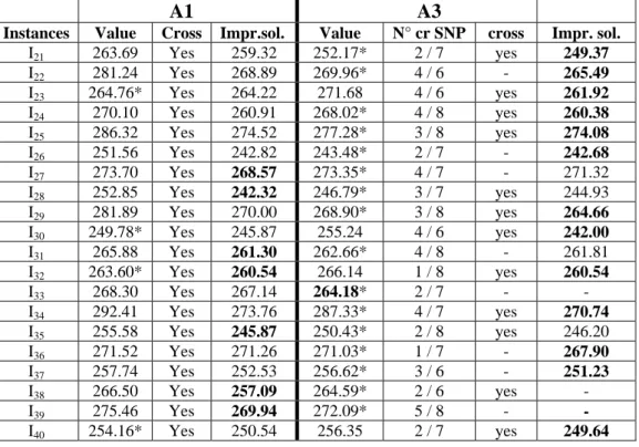
In all the tables, the value of the best solution is reported, as well as the presence of intersections. The symbol * denotes which, between A1 and A3, before improvements, is better; in heavy character, the value of the best found solution is indicated. In A3, the number of crossing SNP’s over the total number of SNP’s is also reported.
Table 1. Graphs with 48 nodes, 8 doubles.
A1 A3
Instances Value Cross Impr.sol. Value N° cr SNP cross Impr. sol.
I21 263.69 Yes 259.32 252.17* 2 / 7 yes 249.37 I22 281.24 Yes 268.89 269.96* 4 / 6 - 265.49 I23 264.76* Yes 264.22 271.68 4 / 6 yes 261.92 I24 270.10 Yes 260.91 268.02* 4 / 8 yes 260.38 I25 286.32 Yes 274.52 277.28* 3 / 8 yes 274.08 I26 251.56 Yes 242.82 243.48* 2 / 7 - 242.68 I27 273.70 Yes 268.57 273.35* 4 / 7 - 271.32 I28 252.85 Yes 242.32 246.79* 3 / 7 yes 244.93 I29 281.89 Yes 270.00 268.90* 3 / 8 yes 264.66 I30 249.78* Yes 245.87 255.24 4 / 6 yes 242.00 I31 265.88 Yes 261.30 262.66* 4 / 8 - 261.81 I32 263.60* Yes 260.54 266.14 1 / 8 yes 260.54 I33 268.30 Yes 267.14 264.18* 2 / 7 - - I34 292.41 Yes 273.76 287.33* 4 / 7 yes 270.74 I35 255.58 Yes 245.87 250.43* 2 / 8 yes 246.20 I36 271.52 Yes 271.26 271.03* 1 / 7 - 267.90 I37 257.74 Yes 252.53 256.62* 3 / 6 - 251.23 I38 266.50 Yes 257.09 264.59* 2 / 6 yes - I39 275.46 Yes 269.94 272.09* 5 / 8 - - I40 254.16* Yes 250.54 256.35 2 / 7 yes 249.64
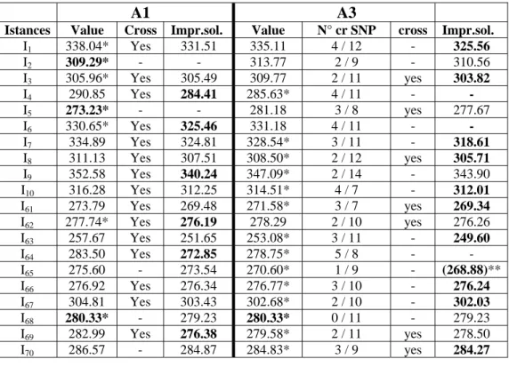
Table 2. Graphs with 48 nodes, 16 doubles.
A1 A3
Istances Value Cross Impr.sol. Value N° cr SNP cross Impr.sol.
I1 338.04* Yes 331.51 335.11 4 / 12 - 325.56 I2 309.29* - - 313.77 2 / 9 - 310.56 I3 305.96* Yes 305.49 309.77 2 / 11 yes 303.82 I4 290.85 Yes 284.41 285.63* 4 / 11 - - I5 273.23* - - 281.18 3 / 8 yes 277.67 I6 330.65* Yes 325.46 331.18 4 / 11 - - I7 334.89 Yes 324.81 328.54* 3 / 11 - 318.61 I8 311.13 Yes 307.51 308.50* 2 / 12 yes 305.71 I9 352.58 Yes 340.24 347.09* 2 / 14 - 343.90 I10 316.28 Yes 312.25 314.51* 4 / 7 - 312.01 I61 273.79 Yes 269.48 271.58* 3 / 7 yes 269.34 I62 277.74* Yes 276.19 278.29 2 / 10 yes 276.26 I63 257.67 Yes 251.65 253.08* 3 / 11 - 249.60 I64 283.50 Yes 272.85 278.75* 5 / 8 - - I65 275.60 - 273.54 270.60* 1 / 9 - (268.88)** I66 276.92 Yes 276.34 276.77* 3 / 10 - 276.24 I67 304.81 Yes 303.43 302.68* 2 / 10 - 302.03 I68 280.33* - 279.23 280.33* 0 / 11 - 279.23 I69 282.99 Yes 276.38 279.58* 2 / 11 yes 278.50 I70 286.57 - 284.87 284.83* 3 / 9 yes 284.27
** In this instance, a not eliminable intersection was present: an ‘intelligent’ exchange was successful (after the transfer, the visit order also was changed!).
Table 3. Graphs with 48 nodes, 24 doubles.
A1 A3
Istances Value cross Impr sol. Value N° cr SNP cross impr sol.
I41 302.53* yes 301.47 306.57 3 / 11 yes 304.66 I42 330.08* - - 333.30 2 / 12 yes 320.20 I43 315.00* - - 315.00* 0 / 13 - - I44 303.89 yes 302.06 303.13* 1 / 10 yes 301.70 I45 282.92 yes 278.57 279.86* 2 / 12 yes 278.80 I46 305.31 yes 303.55 300.73* 3 / 11 yes 300.13 I47 323.27 yes 321.70 321.06* 3 / 15 yes - I48 320.46 yes 316.29 310.04* 4 / 10 yes 309.42 I49 336.63* yes 333.31 338.68 2 / 14 yes 331.85 I50 312.66* - - 312.66* 1 / 12 - - I51 340.21 yes 338.34 337.22* 2 / 13 - 336.27 I52 323.53* yes 322.80 323.77 1 / 13 yes 322.80 I53 332.87* - - 334.15 1 / 11 - 332.00 I54 319.73* yes 316.00 320.49 3 / 12 - - I55 339.27 - - 338.37* 1 / 12 yes 335.07 I56 299.61 yes 298.89 296.96* 1 / 14 - 294.76 I57 316.40* - - 319.54 3 / 10 yes 318.65 I58 308.79 - - 307.05* 2 / 12 - 302.46 I59 315.49* - - 315.49* 0 / 11 - - I60 328.41 yes 326.99 323.84* 4 / 12 yes 323.17
In all the three groups of instances, A3 performs better than A1: this happens more sensibly in the case with lesser double nodes. After the improvement phase, A3 is once more the best algorithm, at a lesser degree in the first and second environment. The extent of the improvement is not generally very high, but sometimes it reach 6%: it is generally higher in A1 than in A3 and in the scenario with lesser double nodes. It should be noted also the very high number of instances in which, after the first phase, in both algorithms the solution has intersections. This is more evident in the algorithm A1 and 8 or 16 double nodes.
5. Conclusions.
In this paper a new algorithm to solve the 2-period balanced travelling salesman problem is presented. Its performance, which is better in the average with respect to other heuristic techniques, is also studied in 60 random instances. The algorithm gives a solution which in most cases can be improved by exchange techniques. The underlying problem is still open, since a tight lower bound on the solution value is not yet known.
6. References.
[1] T. Bassetto, F. Mason (2007) “The 2- period Balanced Traveling Salesman Problem”. Working Paper Series, Dept of Applied Mathematics, Venice University in Ca’ Foscari, n.154.
[2] M. Butler, H.P. Williams, L-A.Yarrow (1997) “The two-period travelling salesman problem applied to milk collection in Ireland”.
Computational Optimization and Applications 7 n° 3, 291 – 306.
[3] J.P. Norback, R.F. Love (1977) “Geometric approaches to solving the travelling salesman problem”. Management Science 23 n° 11, 1208-1223.