A Week in the Life of Three Large
Wireless Community Networks
Leonardo Maccaria, Renato Lo Cignoa,∗
aDISI, University of Trento
Abstract
Wireless Community Networks (WCNs) are created and managed by a local community with the goal of sharing Internet connec-tions and offering local services. This paper analyses the data collected on three large WCNs, ranging from 131 to 226 nodes, and used daily by thousands of people. We first analyse the topologies to get insights in the fundamental properties, next we concentrate on two crucial aspects: i) the routing layer, and ii) metrics on the centrality of nodes and the network robustness. All the networks use the Optimized Link State Routing (OLSR) protocol extended with the Expected Transmission Count (ETX) metric. We analyse the quality of the routes and two different techniques to select the Multi-Point Relay (MPR) nodes. The centrality and robustness analysis shows that, in spite of being fully decentralized networks, an adversary that can control a small fraction of carefully chosen nodes can intercept up to 90% of the traffic. The collected data-sets are available as Open Data, so that they can be easily accessed by any interested researcher, and new studies on different topics can be performed. WCNs are just an example of large wireless mesh networks, so our methodology can be applied to any other large mesh network, including commercial ISP networks.
Keywords: mesh networks, community networks, wireless ad-hoc networks, network topology, privacy, network analysis, centrality metrics, robustness analysis.
1. Introduction
A Wireless Community Network (WCN) is a wireless mesh network created by a local group of users to have an alternative, self-managed, community-based networking infrastructure. A WCN serves two purposes: It allows inter-user interactions (messaging, talking, sharing etc.), and it brings Internet connec-tivity where it is not present. WCNs are flourishing. Many Eu-ropean cities feature WCNs with hundreds of nodes: in Athens a single WCN includes more than 2,400 nodes, while in Spain, the Guifi network is a composition of WCNs that counts more than 23,000 nodes and growing. Thousands of nodes connect-ing tens of thousands of individuals, families, associations, pub-lic offices with a non-profit approach and a community-based organization. After an initial interest in their early stages [1], WCNs have lately re-attracted the attention of academia and research funding [2, 3], and they are becoming a strong asset in reducing the digital divide and pushing broadband networks from the bottom up.
The goal of this paper is to analyze the main features of three large European WCNs, with particular focus on routing aspects and on centrality and robustness metrics.
IThis work is partially funded by The Trentino programme of research,
training and mobility of post-doctoral researchers, incoming Post-docs 2010, CALL 1, PCOFUND-GA-2008-226070, and by the European Commission un-der Grant Agreement No. FP7-288535 “CONFINE”: Open Call 1, Open Source P2P Streaming for Community Networks –OSPS–
∗
Corresponding Author
Email addresses: [email protected] (Leonardo Maccari), [email protected] (Renato Lo Cigno)
1.1. Contribution
This paper extends the initial findings on a small portion of the data presented in [4], leveraging the analysis, the metrics and theoretic contributions published in [5, 6]. It offers an origi-nal combination of insights not present in the existent literature. First of all, three different large networks are monitored for an entire week, exploring their stability and different characteris-tics and finally providing a novel comparative analysis of the three networks.
Second, WCNs do not strictly focus on Internet connectiv-ity, as the large commercial networks analyzed in the literature. Instead, the participants of a WCN perceive the network as an alternative communication media that offers a higher degree of privacy and neutrality. For this reason they try to use the inter-nal services of the network as an alternative to exterinter-nal commer-cial services. In the light of the recent world-wide discussions on privacy, neutrality and forced disconnections, WCNs rep-resent successful networks based on a somehow revolutionary societal approach. For this reason it is particularly important to study their development, describe their features and verify how much they match the expectations, raised even by mainstream media1. One of the contributions of this paper is the analysis
of the robustness and of the centrality metrics of WCNs, that give an unbiased overview of how much these expectations are reflected in real networks.
Third, we focus on specific issues that have been ignored by previous works, as the analysis on the choice of Multi-Point 1See, for instance, recent coverage from the New York Times “U.S.
Relays (MPRs) in the Optimized Link State Routing (OLSR) protocol. MPRs are key nodes used in the OLSR protocol that have been largely debated in the literature, most of the times using a theoretical or simulative approach. We believe this is the first attempt to evaluate on real topologies how MPRs could impact the performance not only in terms of signalling, but also in terms of accuracy in finding the best routes.
Finally, and contrarily to the majority of the works in litera-ture, we release all the data we have collected and the software we developed to encourage more researchers to investigate on this topic, so that new comparative research can be based on this work. We will continue to monitor the three networks and, if possible, to extend the monitoring to new ones and enrich the public data-set with new features2.
1.2. Related Work
Several works describe the features of wireless mesh net-works. In some cases, detailed analysis were made on small wireless networks [7, 8], in some other cases large networks providing Internet access were analyzed [9, 10, 11]. Never-theless, there is a great difference between a commercial ac-cess network and a large WCN, which offers some unique chal-lenges [12] and displays some unique features.
Recently the topological properties of Guifi have been stud-ied [13], and in a previous work [4] we analysed some feature of the Ninux network.
This paper goes beyond the state of the art and focuses on some currently unexplored specific issues. Among these, we will study the centrality metrics applied to WCNs, and, specifi-cally, group centrality metrics. These are metrics that have been largely used in social science, but have been applied to wireless networks only recently [14, 15], but never to networks as large as the ones we consider.
Finally, many works in the literature address the problem of finding the optimal MPR set for a network [16, 17, 18, 19]. Most of these works are based on geometric evaluations or sim-ulations and, to the best of our knowledge, there is none es-timating the impact of different MPR choice strategies in real large topologies as we do in this work.
2. Overview of the Networks and the Measurements The three networks we consider are Funk Feuer Wien and Funk Feuer Graz in Austria, and Ninux in Italy: FFWien, FF-Graz, and NNX for short. They have different management structures and “philosophy”, but they all exploit the OLSR rout-ing protocol to maintain the network topology and compute routing.
2.1. Nodes’ Configuration
The majority of the nodes use either one of two solutions: i) boxed indoor equipment, or ii) commercial devices for outdoor use.
2The software developed and data-sets collected for this work are available
at http://disi.unitn.it/maccari/CN
In the first case devices such as the TP-Link TL-wr841nd3 are modified using outdoor antennas, powered over Ethernet and enclosed in a plastic box. This is a low cost solution, easy to deploy since it relies on omnidirectional antennas that do not need to be aligned. The drawbacks are short ranges, higher in-terference, and a lower throughput.
In the second case devices such as the Ubiquiti nanostation4
are used. They have embedded panel antennas with a beam-width of 40 degrees or parabolic antennas with a beam-beam-width of 10 degrees. This second solution needs more expertise to be installed, but guarantees longer ranges and higher bit rates. Using directional antennas, it is often necessary to install more than one device to connect to neighbor nodes. Each device is connected to the others via Ethernet; this configuration is called a super-node. A super-node implements cross-AP routing and maintains a large horizontal ‘virtual’ coverage angle while fea-turing long ranges and high bit rates.
The communication technology used is a mixture of IEEE 802.11g/a/n standards with preference for 802.11n to achieve higher bit rates and use the 5GHz frequency that is generally less crowded of consumer devices.
Each WCN or user, decides what is the best Operating Sys-tem (OS) for the nodes, and the choice depends on many fac-tors. As a general rule, using the OS shipped with the device has higher stability and better performance due to a better inte-gration with the hardware. As a drawback it may not allow the users to modify the routing protocols or use the ad-hoc mode. 2.2. The OLSR routing protocol
Some comprehension of the OLSR protocol is needed to bet-ter understand the remaining of the paper. Since OLSR is well known and described in the literature [20], we give just a brief description of its principles. OLSR is a link state protocol based on Djikstra algorithm, where only bi-directional links are in-cluded in the link set, and they are discovered using a “hello” procedure that pairs beacons, called HELLO messages, broadcast by each and every node in the network.
Let’s now introduce some specific notation. In a network N each node j has a set of one-hop neighbors N1( j) reachable with
a direct link and discovered with the hello procedure. Nodes are included in N1( j) only if they have proper symmetric links.
Ev-ery node j also has a set of two-hop neighbors N2( j) reachable
through some node i ∈ N1( j) with exactly two hops (by
con-struction N1( j) ∩ N2( j)= ∅).
N1( j) and N2( j) are built as follows: every node j
period-ically sends an HELLO message to build the knowledge about the 1-hop neighborhood. Furthermore, HELLO messages con-tain the IP addresses of every node in N1( j). Through the HELLO
messages of its neighbors, at steady state, j has the full knowl-edge of N1( j) and N2( j).
Node j elects, among the nodes in N1( j), a set of MPRs M( j).
M( j) satisfies the following condition: every node in N2( j) must
have at least a symmetric link towards a node in M( j). Thus if
3See www.tp-link.com/en/support/download/?model=TL-WR841ND 4See www.ubnt.com/airmax
i ∈ M( j) it “covers” some of the nodes in N2( j): M( j)
com-pletely covers N2( j). When j selects one MPR i it informs i
that it has become one of is MPR selectors. Each MPR starts behaving as follows:
• It periodically generates Topology Control (TC) messages. A TC contains the list of the IP addresses of its MPR se-lectors;
• It rebroadcasts the TCs received from its selectors. TC messages contain an approximation of the local topology around an MPR and are received by all the nodes, given the construction procedure of N1( j), N2( j), and M( j). In this way,
each node has enough information to compute the shortest path route to any other node. Since only MPR nodes retransmit the TCs, TCs will reach all the nodes in the network using a fraction of re-transmissions compared to plain flooding. Minimizing the size of each M( j) is thus important to minimize the union of all the M( j), which in turn minimizes the number of generated and forwarded TC messages.
In the network under consideration OLSR is configured to use a quality metric on links: the Expected Transmission Count (ETX) metric. ETX estimates the average number of times a packet needs to be transmitted to reach a neighbor, taking into account losses due to collisions and interference. Since the timer used between every HELLO message is known, each node jestimates the number e of HELLO messages that it should re-ceive from one neighbor i in a given time window. Node j counts the number r of HELLO messages actually received from i in the window and specifies in its HELLO messages the ratio r/e. The value r/e is called the link quality (LQ) of the link from i to j. Node i will do the same, so that node j knows both the LQ value and the reverse value (neighbor link quality, NLQ). Since any unicast transmission in 802.11 requires a data frame and an ACK in the opposite direction, the probability of successfully sending a packet is approximated by LQ × NLQ. The average number of frames needed to successfully send a packet is thus estimated as ET X = 1
LQ × NLQ. MPRs add to the TC messages the ETX for each of their selectors. If ETX is used, the minimum cost route is computed with Dijkstra’s al-gorithm on a weighted graph. Since TC messages contain the ETX metric only for the links between an MPR and its selec-tors, j has only an approximated knowledge of the network. In practice, MPRs hide the presence of some links.
The advantage of using MPRs to reduce overhead, as well as the utility of the ETX metric is hotly debated among OLSR users. Without entering the debate, we note that ETX is a very crude metric and it is estimated on short messages sent in broad-cast, i.e., at the minimum physical transmission speed, which means that ETX is hardly representative of the actual quality of the unicast link between two nodes. It is instead meaningful to estimate the diffusion of routing signalling messages.
2.3. The Data Gathering Process
The data collection relies on the information exposed by the OLSRd daemon. For each community network we store snap-shots of the topology as a weighted non-directed graph G(N, L)
at regular time intervals. N is the set of all nodes, with super-nodes counting as a single node, and L is the set of all links li j
as selected by OLSR. The weight cl∀l ∈ L is either 1 for
mini-mum hop routing or the OLSR ETX metric measured on l. Let Pi, jbe the best path from node i to node j as selected by OLSR
and
w(Pi, j)=X
l∈Pi, j
cl (1)
be its cost or weight.
In all the networks, OLSR is configured to force each node to select all its neighbors as MPRs. As a result every node is an MPR and thus every node has a complete knowledge of the topology. To know the entire topology, it is sufficient to extract information from one node. The OLSRd software daemon can be configured to export the network topology, and all the net-works publish this information. Appendix A describes in detail how the data is collected and what pre-processing is applied to it to make the topological description of the networks more meaningful.
FFGraz FFWien NNX
first sample 01/07/14 01/07/14 01/14/14 last sample 01/13/14 01/13/14 01/20/14
samples per day 144 288 288
samples time interval 10 min 5 min 5 min
Table 1: Summary of the data-sets collected
The data collection process is performed by a daemon writ-ten in the Python language that downloads new topologies in real time and saves them in an SQL database. As we already mentioned, the source code is published as Open Source, and the database as Open Data, so that any researcher wishing to use the data used for this paper is free to access it.
The data has been collected in a period of one week for each network, in Table 1 we report a summary of the data collected for each network. The number of samples of FFGraz is smaller due to the larger sampling period, so that for a one-day obser-vation we have 288 samples for FFWien and NNX and 144 for FFGraz.
3. Main features of the networks
Table 2 shows the key features of the networks. We can note that the three networks are different, but share some topolog-ical characteristics. The NNX network is the smallest of the three, FFGraz is the one with the highest density (the density of a graph G(N, L) is defined as δ = 2||L||
||N || ∗ ||N − 1||). The density in a graph with constant connectivity degree decreases with the number of nodes, so even if NNX has a smaller average degree compared to FFWien, it has a higher density. The pro-portion between leaf nodes and non-leaf nodes is similar in the three networks. Another measure of interest is the average local clustering coefficient of the network (CC1), that expresses the
FFGraz FFWien NNX
av. number of nodes 144 236 131
av. number of links 207 421 153
density δ 0.020 0.015 0.017
average degree 2.88 3.63 2.35
leaf nodes 63 (43%) 77 (32%) 51 (38%)
average ETX 2.0 1.46 1.24
average CC1 0.1934 0.2358 0.0347
Table 2: High level features of the networks under analysis
local density of links around a node. The local clustering coef-ficient of node i with one-hop neighborhood size ni= |N1(i)| is
defined as: CC1(i)=
2|{lk, j: k, j ∈ N1(i) ∧ lk, j∈ L}|
ni(ni− 1)
(2) In average, Ninux has a much smaller CC1compared to Funk
Feuer Graz and Funk Feuer Wien. 3.1. Time Evolution of the Networks
During the observation on the whole week we measured only a small fluctuation in the number of nodes and in the number of links, mainly due to a small subset of leaf nodes with instable links that periodically exit and enter the main connected com-ponent of the network. This is reported in Fig. 1 where one snapshot per hour for the full week is reported. Note that the fluctuations of leaf nodes/links (the upper plot) have a marginal impact on topology and routing.
Fig. 2 reports the persistence of each link of the networks, that is, the fraction of snapshots over the total for which the link has been present in the network. From this data we removed the links that have a persistence smaller than 1%. This is to avoid to consider sporadic links generated by test devices or tempo-rary changes in the nodes configurations. There is a difference among the networks, while NNX shows a very high persistence for the majority of the links, FFWien and FFGraz present more temporary links. Still, in both cases there is a large core of links that is present in all the snapshots.
The fluctuation of the number of nodes and links does not impact the macroscopic routing characteristics of the topology. The reason is that fluctuations normally happens in marginal nodes and links, so that the average length and cost of the short-est paths are not influenced. This observation is reported in Fig. 3, together with the average ETX, which doesn’t vary sig-nificantly, either.
Fig. 4 reports the clustering coefficient of each network. Sect. 5 discusses how CC1directly influences the robustness of
the networks.
Since the network features are stable, from now on we limit the analysis to data relative to one day of observation, in order to reduce the effects of fluctuations and simplify the interpretation of results. Since the full data-set is available on-line, all the results are reproducible also for other time-periods. We have observed some other days obtaining consistent results.
0 10 20 30 40 50 Snapshot 100 150 200 250 N od es
FFGraz ninux FFWien
100 200 300 400 500 Li nks 60 65 70 75 80 85 Le ave s
Figure 1: The number of nodes, leaves and edges for the three networks during the whole week.
0 50 100 150 200 250 300 350 0.0 0.5 1.0 Persistence FFGraz 0 20 40 60 80 100 120 140 160 0.0 0.5 1.0 ninux 0 100 200 300 400 500 600 700 link 0.0 0.5 1.0 FFWien
Figure 2: Persistence of the links for each network
3.2. ETX and Degree Analysis
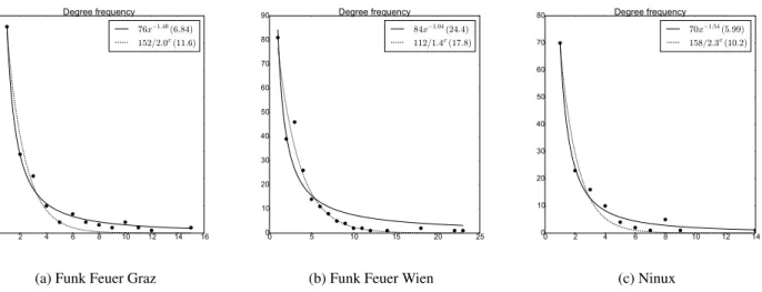
Fig. 5 shows the average degree distribution of the three net-works. For each node the degree is averaged over all the snap-shots and rounded to the closest integer. The figure reports also the power law and exponential curves that best fit the points (using minimum mean square error). Since the number of sam-ples and the dimension of the network are not large enough to compare it with existing literature on power-law networks, we do not indulge in the analysis of the degree distribution; we just observe that qualitatively the distributions are very skewed. This is not surprising also considering the results on another WCN presented in [13].
Fig. 6 shows the empirical CDF of ETX for all the links and all the snapshots. A large portion of the links have an ETX ' 1. Independently from the network the distributions have a long tail of higher values, but the slope is different. Fig. 7 reports the average ETX for every link computed on all the snapshots. In 4
0 2 4 6 8 10 12 14 16 0 10 20 30 40 50 60 70 80 Degree frequency 76x−1.40(6.84) 152/2.0x(11.6)
(a) Funk Feuer Graz
0 5 10 15 20 25 0 10 20 30 40 50 60 70 80 90 Degree frequency 84x−1.04(24.4) 112/1.4x(17.8)
(b) Funk Feuer Wien
0 2 4 6 8 10 12 14 0 10 20 30 40 50 60 70 80 Degree frequency 70x−1.54(5.99) 158/2.3x(10.2) (c) Ninux
Figure 5: Degree distributions with exponential and power law fitting curves
0 10 20 30 40 50 Snapshot 1.0 1.5 2.0 2.5 ET X
FFGraz ninux FFWien
4.5 5.0 5.5 6.0 R ou te L en gt h 5 6 7 8 9 10 R ou te W ei gh t
Figure 3: Average ETX value, route length, and route weight for the three networks during the whole week
0 10 20 30 40 50 Snapshot 0.00 0.05 0.10 0.15 0.20 0.25 0.30 Cc
FFGraz ninux FFWien
Figure 4: Clustering Coefficient for the three networks during the whole week
Ninux it has a smaller range compared to Funk Feuer networks. In all networks and all links ETX is relatively stable: the
av-0 2 4 6 8 10 ETX 0.0 0.2 0.4 0.6 0.8 1.0 Pro ba bi lit y FFGraz ninux FFWien
Figure 6: ECDF of the ETX value for the three networks
0 100 200 300 400 500 link 1 2 3 4 5 6 7 8 9 10 ET X FFGraz ninux FFWien
Figure 7: Average ETX of each link in the three networks (links are ranked by ETX)
erage standard deviation of the ETX on each link is less than 16%, 10% and 7% for Funk Feuer Graz, Funk Feuer Wien and
Ninux respectively. This actually contradicts the common as-sumption that in WCNs the links are unstable and their quality is highly variable.
In the past, due to the unavailability and price of devices, the networks were set-up using omnidirectional antennas, and ad-hoc wireless mode. This allowed maximum flexibility, almost no planning, but it also yielded poor performance and high in-terference. Today, a large number of nodes are equipped with directional antennas, and the super-node configuration (see Ap-pendix A) is used to enlarge the coverage angle of each node. In some cases the original firmware is not changed on the radio device, and master-client configurations are used. This requires some effort in network planning, but it also allows the use of proprietary extensions that further increase the performance of each link. In the case of Ninux we verified these assumptions directly with people from the WCNs that confirmed that the majority of the nodes are configured to have one link per each radio.
We note some differences. Ninux has the best average qual-ity, and more than 90% of the links have ETX ≤ 2, while Funk Feuer Graz has the highest average ETX and the highest stan-dard deviation per link; it is the one with the highest density, suggesting that in Funk Feuer Graz it is more common to to use the same device for more than one link.
4. The Routing Layer
Once the weighted network graph is known, we can compute all the shortest paths from any couple of nodes in the network. Since every node is an MPR this is the same information that a node in the network uses to compute its routing table.
Fig. 8 reports the distribution of the paths’ weight w(Pi, j)
computed both with a simple hop-count metric (cl= 1 ∀l ∈ L)
and considering the ETX metric as OLSR does. The graph is based on all the routes computed on all the snapshots of a one-day data-set. w(Pi, j) is quantized to integer values for readabil-ity.
Funk Feuer networks have the mode at 5 hops, while Ninux despite being the smallest of the three has the mode at 6 hops (this can be explained observing that it is the network with the smallest average degree). The difference between the curves representing length and weight can be better appreciated look-ing at the cumulative distribution. In Funk Feuer Wien and Ninux the curves are very close to each other, while in Funk Feuer Graz the difference is much more evident. This shows that the highest quality of the links in Funk Feuer Wien and Ninux is directly reflected in the paths’ weight w(Pi, j) computed on ETX. Notice that Funk Feuer Graz features a very different distribution of w(Pi, j) computed on ETX compared to the other networks. The reason lies in the particular topology that leads to some nodes with high centrality but bad links and will be more clear after the discussion in Sect. 5. Fig. 10 shows a snap-shot of the Funk Feuer Graz topology where, albeit only with a trained eye, this somewhat pathologic situation can be seen.
Fig. 9 reports boxplots of w(Pi, j) ∀i, j based on ETX grouped by number of hops, and computed in each network, for each
Figure 10: Compressed Funk Feuer Graz topology, the number in circles indi-cates the number of attached leaves. The density of the link color is proportional to its goodness (light blue= bad link). 3 clusters can be identified, two of them connected with weak links.
snapshot. The boxplots show some intuitive but interesting re-sults. For the FFWien and NNX networks the median of the weights (the red line in the box) is very close to the minimum value (the bottom whisker). Also, the first and third quartile (the boxes) are close to each other, which means that more than 75% of the routes of the same length have a very similar behaviour. In FFWien with routes longer than 6 hops the upper whisker starts diverging from the median, indicating a higher variance of w(Pi, j). This is not evident in the Ninux network. In FF-Graz there are two separate effects, the first one is that even for shorter paths the boxes are much wider than for the other net-works, the second is that, due to the particular topology of the network, the variance of w(Pi, j) is not monotonic.
As a concrete application of this analysis, imagine that a cer-tain service is placed on a single node i in the network, and must be reached by any other node j, for instance, a VoIP Bor-der Media Gateway. The weight w(Pi, j) influences the service quality since it is an estimate of the average number of wireless frames that need to be sent along the path for the packet deliv-ery. In Ninux if i is chosen to be at an average distance of 6 hops from any j (the mode of the route length as seen in Fig. 8c) the perceived quality of the service will be similar for the large ma-jority of nodes since the boxplots for length 6 is narrow. This is not true for FFGraz, for which, among the routes that have a length 5 (the mode for FFGraz) the distribution of the weights is much wider. Thus the perceived quality of the service will largely differ depending on the position of j. Since the average distance of i from any node j can not be arbitrarily reduced, the only solution to have a more homogeneous quality is, if possi-ble, to use two servers, thus doubling the effort. Other similar issues will be discussed in Sect. 5.
4.1. Analysis of the Multi-Point Relays
The distinctive feature of OLSR, and one of the most de-bated, is the way MPRs are selected [16]. We introduce some 6
1 3 5 7 9 11 13 15 17 19 21 23 25 ETX weight/hop count
0.00 0.05 0.10 0.15 0.20 R el at ive F re qu en cy 0.0 0.2 0.4 0.6 0.8 1.0 Pro ba bi lit y
Frequency of route length and weight, FFGraz
Weight ECDF Weigth Distribution Length ECDF Length Distribution
(a) Funk Feuer Graz
1 3 5 7 9 11 13 15 17 19 21 23 25
ETX weight/hop count 0.00 0.05 0.10 0.15 0.20 0.25 R el at ive F re qu en cy 0.0 0.2 0.4 0.6 0.8 1.0 Pro ba bi lit y
Frequency of route length and weight, FFWien
Weight ECDF Weigth Distribution Length ECDF Length Distribution
(b) Funk Feuer Wien
1 3 5 7 9 11 13 15 17 19 21 23
ETX weight/hop count 0.00 0.02 0.04 0.06 0.08 0.10 0.12 0.14 0.16 0.18 R el at ive F re qu en cy 0.0 0.2 0.4 0.6 0.8 1.0 Pro ba bi lit y
Frequency of route length and weight, ninux
Weight ECDF Weigth Distribution Length ECDF Length Distribution
(c) Ninux
Figure 8: Empirical distribution (solid lines, left y axis) and ECDF (dashed lines, right y axis) w(Pi, j) based on hop count (green/thin line) and ETX (blue/thick line)
(a) Funk Feuer Graz (b) Funk Feuer Wien (c) Ninux
Figure 9: Boxplots of the distribution of w(Pi, j) vs the number of hops in the path; boxes represent the 1st and 3rd quartile, the whiskers are set to 1.5 times the Inter Quantile Range. X axis reports also the percentage of routes with the corresponding length
notation to further discuss this subject. Let j be a node of the network, N1( j) is its neighbors’ set and M( j) ⊆ N1( j) is the set
of MPRs chosen by j, Mgis the union of all M( j); Sg = ||Mg||.
S(i) is the selector set of MPR i and the symbol j → i means j ∈ S(i).
As a general policy, Sg should be small, since every MPR
generates signalling that is propagated to all nodes. The heuris-tic proposed in the OLSR RFC tries to minimize each M(i), and it has been shown that it produces results close to the lo-cal optimum in dense scenarios [20, 21]. Minimizing also the intersection of each M(i) reduces Sgeven further [19].
Com-pletely decoupling the choice of M(i) from the links’ quality may lead i to choose an MPR j even if the ETX on the link is high (bad link). This has two drawbacks. The first is the poten-tial computation of sub-optimal paths. As each node has only an approximated view of the network based on HELLO and TC messages, an Mgbuilt ignoring quality metrics may hide (as we
explained in Sect. 2.2) links with high quality, and lead to com-pute sub-optimal routes (we call this conjecture [A], as it is one of the assumptions upon which many decisions and choices are
taken in tuning OLSR, but rarely verified). The second is that the robustness of the diffusion of signalling may be reduced. In fact, i may not receive TCs from j and thus have outdated infor-mation on the network topology (conjecture [B], also this one an assumption often made, but rarely verified).
The OLSRd community has initially implemented its own quality-aware MPR selection algorithm that chooses for each 2-hop neighbor the 1-hop neighbor that maximizes the quality on the two-hop path, an idea initially introduced in [22]. Con-sequently Mg in a dense network constantly changes, since it
doesn’t depend on the links availability, that is assumed to be slowly changing, but on the link quality that can be much more variable. A fast changing Mgcan have two bad consequences.
The first one is that also the routing may be changing frequently. When Pi, jchanges, even if w(Pi, j) remains similar, other quality
parameters of the route can vary (for instance, ETX doesn’t esti-mate the capacity of a link). The protocols and the applications at the upper layers can be highly impacted by such variations. The second one is that every time there is a change in Mgthe
HELLO and TC messages. When the information propagation time becomes comparable to the time between changes there is a high risk of network instability. The result of a large period of trial and error [23] was that the developers of OLSRd, as a de-fault configuration, force every node to select all its neighbors as MPR, in practice renouncing to the optimization introduced by the MPRs. As said, this is also the approach used in the three networks under evaluation.
With the data-set available we can evaluate the impact of different choices of MPRs. The introduction of quality-aware MPRs selection raises many issues and gives many choices, which are often used arbitrarily. We want to study if conjec-tures [A] and [B] justify the use of quality metrics or not and how different MPRs selection influences the topology quality. We call Mgqthe set of MPRs chosen with the link-quality
maxi-mization metric, and Sqgits size.
4.2. Overhead reduction
Since we have the full topology and all clwe can compute
off-line Mg and M q
g reproducing both metrics. Figure 11a and
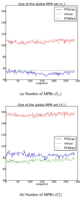
11b report Sgand S q
gvs time (snapshots) for a one-day subset
and show two relevant facts: i) Sgqlargely exceed Sg; and ii) Sg
for FFGraz is smaller compared to NNX, but this is the opposite for Sqg. The reason for ii is that FFGraz is larger and denser
NNX, so that the Sgreduction achievable on FFGraz is higher
(the MPR choice with the RFC heuristic is more efficient in dense networks). In Ninux the physical topology and the low density strongly influences the choice of Mg, and Sgcannot be
reduced.
To quantify how this impacts the signalling overhead, Fig. 11c reports Lt, which estimates the normalized load per
link per generated TC: Lt= Elhρlt
i
; l ∈ L (3)
where El[·] is the average over all links and ρltis the total
num-ber of TCs transmitted on link l in each TC interval. It is clear that reducing Sg is fundamental to reduce the signalling
over-head. FFGraz has an average of 10% more nodes than NNX, but also 35% links more than NNX, this explains why FFGraz has less TC messages per link.
This estimation does not consider TC aggregation or fish-eye strategies, that can reduce the global amount of TC messages re-gardless of MPR selection strategy. Note also that Fig. 11c only reports TC messages, but MPRs are used to re-broadcast any other signalling messages, such as HNA messages, or messages needed to spread the association between a node and a list of its available services. Thus, it is of paramount importance to re-duce the number of MPRs to keep the signalling bearable when the network size grows.
4.3. Route quality
Let’s now analyze the impact of MPR selection on route cal-culation. The base of conjecture [A] is that a node i receives topology information from HELLO and TC messages. Thus, it has only an approximated view of the network. We want to quantify how much this can negatively influences routing.
0 50 100 150 200 250 300 snapshot 40 60 80 100 120 140 160
Size of the global MPR set (Sg) FFGraz ninux FFWien (a) Number of MPRs (Sg) 0 50 100 150 200 250 300 snapshot 40 60 80 100 120 140 160
Size of the global MPR set (Sq g)
FFGraz ninux FFWien
(b) Number of MPRs (Sqg)
FFGraz ninux FFWien
0 20 40 60 80 100 120
140
TC messages per link per TC emission interval
RFC
lq
LSR
(c) Estimated TC load Lt
Figure 11: a) Sgand Sqg. c): TC load Lt(LSR is OLSR without MPR
optimiza-tion, lq uses link-quality based MPR computation) 8
Define Gi(N, L0) as the approximated view of the network
graph G by node i. Gi has the same number of nodes of the
original graph G but has a smaller number of edges. L0 ⊆ L contains the edges lk j for which at least one of the following
condition holds: 1. k= i, or j = i 2. k ∈ N1(i) or j ∈ N1(i)
3. k ∈ Mgand j → k or j ∈ Mgand k → j
In practice, each node i knows only the links to its neighbors, the links between its 1-hop neighbors and its 2-hop neighbors and the link between any MPR in the network and its selectors. For this analysis the MPR are chosen using the heuristic from the RFC, without considering link qualities.
Given Gi we can compute the routing table Ri( j) for every
node i, and hence, for every (i, j) in N × N compute the e ffec-tive path P0
i j= {i = p0, p1 = Rp0( j), p2= Rp1( j) . . . j} that
pack-ets follows from i to j. Comparing w(P0
i j) with w(Pi, j) gives a
measure of the real impact of conjecture [A].
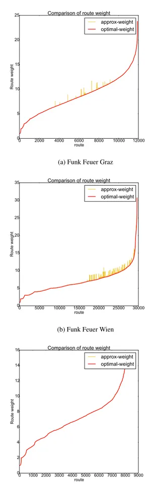
Figs. 12a, 12b, and 12c report w(P0i j) with w(Pi j) for all pairs
(i, j) averaged on all the snapshots and ranked by their weight. Surprisingly enough, the difference is extremely limited, in 98% of the samples the same routes are chosen and the curves overlap. This can be explained observing that even if node i doesn’t have enough information to compute the globally best route, it has enough information to send the packet to the most convenient next-hop. Then, at any hop, the node that is rout-ing the packet has a full knowledge the graph up to its 2-hop neighborhood, and can choose again the most convenient next hop.
This result is particularly relevant considering that OLSR2 [24], which is currently in its final stage of standardization distinguishes between MPRs used to broadcast signalling and MPRs used for routing. This choice was taken because of con-jecture [A]. At least for these three networks, and we believe for WCNs and meshes in general, this difference doesn’t hold: maintaining two sets of MPRs may be an unjustified overhead. OLSR is still one of the most used protocol in WCNs, even if the communities tried to mitigate its limitations creating new protocols, such as BATMAN, that is also widely used [23]. BATMAN, being a distance-vector protocol generates smaller signalling messages, but it doesn’t give a full view of the net-work to each node. We believe that the data we gathered show that a correct implementation of OLSR can greatly reduce the overall signalling, while maintaining stability properties. We also believe that, even if this information is currently not used, the knowledge of the full network topology (or at least of an approximated one) can be beneficial to fine-tune the protocol properties. For instance, the frequency of the signalling could be raised for nodes that prove to be central in the topology, and lowered for nodes that are in the periphery. The next Section shows how to compute centrality metrics within OLSR, some-thing that would be much more difficult to do with a distance-vector routing protocol.
0 2000 4000 6000 8000 10000 12000 route 0 5 10 15 20 25 Ro ute w eig ht
Comparison of route weight approx-weight optimal-weight
(a) Funk Feuer Graz
0 5000 10000 15000 20000 25000 30000 route 0 5 10 15 20 25 30 35 Ro ute w eig ht
Comparison of route weight approx-weight optimal-weight
(b) Funk Feuer Wien
0 1000 2000 3000 4000 5000 6000 7000 8000 9000 route 0 2 4 6 8 10 12 14 16 Ro ute w eig ht
Comparison of route weight approx-weight optimal-weight
(c) Ninux
5. Centrality and Robustness Metrics
In graph theory, centrality metrics have been largely used to identify the properties of nodes. In particular, in social science the centrality of a node is often used to determine the influence that a person has on the other participants of the social network. In the context of wireless networks, centrality has not received much attention up to recent times [14, 15].
The concept of centrality in a specific graph is not unique, in this paper two definitions of centrality are considered, shortest path group betweenness centrality Csp, or simply betweenness,
and group closeness centrality Cc (definitions can be found
in [25]). Computing group centrality is a hard task, so that heuristics must be used for networks of the size we are con-sidering.
Robustness metrics are used, instead, to study the robustness of the network against nodes or link failures. We will quantify the robustness of the network graph, but also introduce an ini-tial evaluation of how the introduction of MPRs can impact the diffusion of TC messages.
5.1. Centrality Metrics
The Csp(k) of node k is defined as the fraction of shortest
paths Pi, j ∀i, j ∈ N passing through k. If the traffic matrix is uniform or unknown, Csp(k) is an unbiased estimator of the
fraction of traffic that a node will route. If one wants to place a traffic analyzer in the network (for instance an Intrusion De-tection System (IDS)), the node with the highest Cspis the best
choice to intercept the highest fraction of the overall traffic. The closeness centrality Cc(k) of node k, instead, is an
esti-mation of the cost needed to spread an inforesti-mation from k to all the nodes in the network. The definition that best serves the purposes of this paper is that Cc(k) is the average distance from
kto any other node i in the network5. If one wants to place a ser-vice in the network (a web server, a streaming server, etc.) the node with the lowest Ccis the best choice to minimize its
dis-tance to any node in the network. For both centrality measures the weighted graph is used, so that distances are weighted us-ing ETX; thus, Cc(k) is the average number of wireless frames
that will be needed to successfully send one IP packet from any node i to the service placed on k (or vice versa).
The definition of both metrics can be extended to groups of nodes. The group betweenness of a group γ of nodes is defined as the fraction of Pi, j ∀i, j ∈ N passing through at least one
node of γ. Again, if one wants to place an IDS on a group γ of nodes in order to maximize the overall fraction of traffic analyzed, the group with the highest Csp(γ) is the best choice.
The closeness group centrality of γ is the average of the min-imum shortest path from any node i to any of the nodes in γ. Among all the groups of the same size, the more central one is the one with the lowest Cc(γ).
5Closeness centrality is generally defined as the inverse of C
c(k). We prefer
to use Cc(k) since coupled with the ETX metric, its value has a direct
correspon-dence with the average number of wireless frames sent along the path from any node i to k.
Following the previous example, if a service can be repli-cated on a set γ of nodes, then the group with lowest Cc(γ) is
the best choice. As a further example imagine that Cc(γ) can be
used as a metric to place Internet gateways. The group with the lowest Cc(γ) is the group that will give the best average Internet
connectivity to the nodes in the network. Since the ETX metric of a link is an estimation of the number of frames needed to successfully deliver an IP packet on that link, Cc(γ) is directly
proportional to the average load (in terms of number of frames) on the network generated by the traffic directed to the Internet. This is of particular importance also for a commercial Wireless ISP that needs to design a mesh network to deliver internet con-nectivity. The number and the position of the gateways in the network must be decided in order to distribute the load on the whole topology and reduce the chances of creating bottlenecks. 5.1.1. Computing Group Centrality
Finding the group γ with the highest group betweenness has been shown to be an NP hard problem while a brief analysis of the literature did not produce any complexity estimation for the closeness group centrality as we defined it.
The size of the networks under consideration does not al-low the use of an exhaustive search on all the groups of size kto find the global optimum, thus we implemented a greedy algorithm we call GR1 to estimate the best group. At each step h, given the solution computed at the previous step γh−1,
for every i in N, GR1 composes a new set γi
h = γh−1 ∪ {i}
and computes µi = Csp(γhi) − Csp(γh−1). It ranks all the γihfor
the corresponding µi and selects the one with highest µi. The
difference from the optimal Csp(γo) and Csp(γk) produced by
GR1 has been shown to be lower bounded by a constant in the general case [26], moreover GR1 performs particularly well on scale free networks [27]. Some of our networks show a scale free behaviour, so we chose this greedy algorithm to compute the best centrality measures. Nevertheless, since our between-ness centrality measure is slightly different from the one used in [26] and closeness centrality was not considered in that work, we validated the greedy algorithm with a GRASP (Greedy Ran-domized Adaptive Search Procedure) approach, and in partic-ular, with a parallel multiple-walk independent-thread proce-dure [28] that we called GR2. GR2 works as GR1, but instead of always choosing the γi
hwith highest µiit selects a restricted
candidate list of the first 5 and randomly picks one of them, with probability proportional to µi. We ran GR2 with 16
in-dependent parallel processes for each network graph and chose the best solution. If the problem we want to solve has many local optimum values far from the global one, GR2 should per-form substantially better GR1. Instead we verified that GR2 produces a negligible improvement in both centrality metrics, less than 1% on average compared to GR1. This confirms that on the topologies of our data-set GR1 produces solutions very close to the optimum.
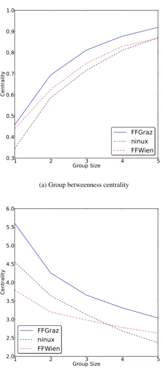
Fig. 13a shows the group betweenness centrality of groups up to size 5. It is clear that a motivated attacker, controlling a few nodes is able to sniff a very large portion of the traffic. In light of the recent Datagate privacy scandal, WCNs have at-tracted the attention of mainstream media as a bottom-up alter-10
1 2 3 4 5 Group Size 0.3 0.4 0.5 0.6 0.7 0.8 0.9 1.0 C en tr al it y FFGraz ninux FFWien
(a) Group betweenness centrality
1 2 3 4 5 Group Size 2.0 2.5 3.0 3.5 4.0 4.5 5.0 5.5 6.0 C en tr al it y FFGraz ninux FFWien
(b) Group closeness centrality
Figure 13: Group Betweenness and closeness Centrality of the best groups with size from 1 to 5
native to avoid privacy infringement6. Our analysis on real net-works shows instead that using a peer-to-peer technology does not guarantee by itself to have networks that are robust to inter-ception.
6See the New York Times, “Home Wireless Network Keeps the Snoops
Away”
http://www.nytimes.com/2013/11/14/technology/personaltech/ homemade-wireless-networks-keep-the-snoops-away.html?smid= pl-share&_r=0
The other side of the coin is that a distributed monitoring sys-tem placed on a small subset of nodes will be able to intercept and analyze the majority of the traffic of the network, and also to counter external attacks to privacy.
Fig. 13b instead shows that with a careful choice of γ the average network load generated by traffic directed to the gate-ways or to a set of servers can be cut down significantly. Re-call that with OLSR, each node exposes the private networks it is connected to using specific messages (HNA messages). By extension, it can also export the offered services (as in [29]). OLSR thus offers an easy and efficient way (since it exploits the MPR system) to spread the knowledge that a particular ser-vice is present in a set γ of nodes. Every other node is thus able to use the service on the host in γ that is more convenient to reach.
5.2. Robustness
The robustness of a graph is an estimation of the impact of failures on the graph connectivity, and can be measured with metrics introduced in [30] and based on percolation theory. Given a connected graph G(N, L) we remove a set F made of f random edges and we call G0(N0, L0) the main connected
component of the resulting graph. When an edge is removed the connectivity of the graph may change, meaning that some nodes can be isolated. The robustness of G(N, L) is the ra-tio ||N||N ||0||, averaged over a sufficient number of random choices of F. The rationale behind this metric is that if the robustness stays close to 1, the network is still functionally behaving as a network when subject to f uncorrelated failures. Instead, if it drops to values close to 0, the network is fragmented into a multitude of isolated networks. In practice, there is no network anymore. The same measure is repeated for growing values of
f.
We compute the robustness of each snapshot with 30 ran-dom choices of F and growing value for f . Instead of express-ing the robustness against the absolute number of failures, it is convenient to express it against relative number of failed links, so that different networks can be compared. Since the number of edges in each snapshot (even of the same network) lightly varies, we quantize the relative number of failures to a percent-age: k= d100 ∗ f /||L||e. Then for each network we call r(k) the robustness averaged over every snapshot.
Since ETX expresses the reliability of a link, instead of choosing the edges with an uniform distribution the probabil-ity of being removed is proportional to the normalized value of ETX.
We choose to compute the robustness in four different ways: 1. On the full graphs;
2. On the full graphs, but choosing the links to purge only within the core network, i.e., only the links that connect non-leaf nodes;
3. On the MPR sub-graph Gm(N, Lm) in which a link exists
only from a selector to its MPR. MPRs are chosen with the RFC heuristic;
4. On the MPR graph Gqm(N, Lq) built as the previous one
The last two ways affect the signalling network only. To better explain this we refer to Gmbut the considerations are the same
for Gqm. When a node m that is not an MPR generates an HELLO
packet to show its presence, this information is distributed to the whole network by at least one MPR i for which m → i. Similarly, when a TC message is produced by i, the information it carries moves from i to any other MPR j for which i → j, and this is repeated at every hop. If one link is broken, TCs can still arrive to every destination using alternative paths. But, if one or multiple failures make Gmdisconnected, the network is
logically broken. If this condition is not transitory, the routing needs to be reconfigured and temporarily some routes will be missing. Computing r(k) on Gm, we give an estimation of how
robust is the delivery of routing information on Gmthat directly
depends on Sgand S q g.
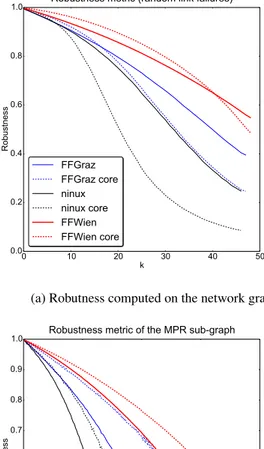
Fig. 14a shows the robustness of the network and of the net-work core. First of all we can observe that all the netnet-works are quite robust. If we remove 10% of links, that is a relevant portion of the links, robustness is higher than 0.9. Second, ro-bustness is higher for networks with higher average degree, and this is particularly evident between FFGraz and NNX. Even if their size is similar, in NNX, the choice of minimizing the num-ber of links per device increasese the average quality per link, but decreases the robustness.
There is a visible difference between the robustness of the full graph and of the core graph. In all three cases, for low values of k the core network is more robust that the full network, then the two curves intersect. To understand this, consider that if we remove a random link, if this link connects a leaf node ||N0|| decreases by one unit. Instead, if the core network is well con-nected, removing one link does not necessarily decrease ||N0||. Since FFGraz and FFWien have a higher degree than NNX the intersection happens for higher values of links removed.
Fig. 14b presents the robustness of the MPR sub-graphs. It is intuitive that Gm will be less robust than G
q
m since it has
a smaller Mg. For this reason we normalize the number of
failed links to the number of MPRs. Thus, we plot r(k0) where
k0 = d100 × f /S
ge, and r(k00) where k00 = d100 × f /S q ge
in-stead of r(k) respectively. This metrics express the robustness normalized to the respective sizes Sqgand Sg, notice that k0and
k00 can be larger than 100, so that they are not normalized pa-rameters strictly speaking, as they are referred to a number of nodes and not to a number of links. As a result we see that the curve referring to quality-based MPR selection (solid lines, marked with “lq” in the figure legend) stays below the curve referring to the standard RFC implementation. This is relevant with respect to conjecture [B]: we can finally say that using the RFC heuristic produces a small reduction in terms of robust-ness, which is largely compensated, from a global management point of view, by the reduction of MPRs, and consequently of signalling, making quality-based MPR selection questionable.
Similarly, robustness can be evaluated against the failure of nodes, simply considering a random set of f nodes, normalized on the size of N. Fig. 15a and Fig. 15b show the robustness of the network graph to the failure of nodes. We evaluate the robustness against random failures and targeted attacks. In the first case, the nodes are randomly removed from the networks,
0 10 20 30 40 50 k 0.0 0.2 0.4 0.6 0.8 1.0 Ro bu stn ess
Robustness metric (random link failures)
FFGraz FFGraz core ninux ninux core FFWien FFWien core
(a) Robutness computed on the network graph
0 50 100 150 200 k' (k'') 0.2 0.3 0.4 0.5 0.6 0.7 0.8 0.9 1.0 Ro bu stn ess
Robustness metric of the MPR sub-graph
FFGraz-RFC FFGraz-lq ninux-RFC ninux-lq FFWien-RFC FFWien-lq
(b) Robutness computed on the MPR sub-graph
Figure 14: Robustness metric for link failures on the network graphs and on the MPR sub-graphs with both RFC and ETX based heuristics
in the second, we start removing nodes from the one that have the highest degree. This second case resembles the actions of a rational attacker that wants to provoke the highest damage to the network.
The graphs show that due to the high skewness of the degree distribution, the networks are quite resistant to random failures, but are pretty weak against targeted attacks.
0 10 20 30 40 50 Failed nodes (%) 0.1 0.2 0.3 0.4 0.5 0.6 0.7 0.8 0.9 1.0 Ro bu stn ess
Robustness metric (random node failures) FFGraz ninux FFWien
(a) Robustness to random node failures
0 10 20 30 40 50 Robustness 0.0 0.2 0.4 0.6 0.8
1.0 Robustness metric (targeted attack on nodes) FFGraz ninux FFWien
(b) Robustness to targeted attacks
Figure 15: Robustness metric for node failures
6. Conclusions
Wireless Community Networks represent a thriving mix of technical solutions and social participation. Their open nature allows users and researchers to participate, experiment and col-lect information on how the networks work. In this paper we used the data collected on three large WCNs to study their main topology features, the centrality of their nodes and their robust-ness. We also used the data-set to investigate on the role of MPRs in an OLSR-based network, something that, to the best of our knowledge, has never been done on such a large scale. The results show that, even with some differences, WCNs are pretty stable networks, the average quality of the links is good, and thus, the weights on the routes are close to their length in terms of hops. We also showed that the use of MPRs can re-duce the signalling, without a strong impact on the quality of the routes.
WCNs are often perceived as a tool that users can build to escape control and protect their privacy. We showed that the structural properties of the networks alone do not make them more robust against coordinated attacks, since the traffic is con-centrated on a few important nodes (as we showed using cen-trality metrics) and the connectivity relies on a few important nodes (as we showed using robustness metrics).
A preliminary version of the data-set and of the code used for the analysis is already available for public use and the pos-sible falsification of our results. We are actively documenting the code used and improving its usability and the access to the database as full Open Data7.
Many further research topics can be explored on the data-set, for instance, we plan to study the properties of the most cen-tral nodes, verify how much they change with time and how we can use heuristics to avoid the complex algorithms we have used in our analysis. Central nodes may behave differently (for instance, their signalling can be more frequent) and the rout-ing protocol could take advantage of the knowledge of the full topology, contrarily to what happens now.
7. Acknowledgemts
We greatly thank all the people from the community net-works that contributed to the gathering of the data. In partic-ular, Aaron Kaplan and Ralf Schlatterbeck for the Funk Feuer networks and Claudio Pisa for the Ninux network.
Bibliography
[1] S. Jain, D. Agrawal, Wireless community networks, IEEE Computer 36 (8).
[2] P. Frangoudis, G. Polyzos, V. Kemerlis, Wireless community networks: an alternative approach for nomadic broadband network access, IEEE Communications Magazine 49 (5).
[3] A. Neumann, I. Vilata, X. Le´on, P. E. Garcia, L. Navarro, E. L´opez, Community-lab: Architecture of a community networking testbed for the future internet, in: IEEE International Conference on Wireless and Mo-bile Computing, Networking and Communications (WiMob), Barcelona, Spain, 2012.
[4] L. Maccari, An analysis of the ninux wireless community network, in: IEEE International Conference on Wireless and Mobile Computing, Net-working and Communications (WiMob), Lyon, France, 2013.
[5] L. Maccari, R. Lo Cigno, Waterwall: a cooperative, distributed firewall for wireless mesh networks, EURASIP Journal on Wireless Communica-tions and Networking 2013 (1).
[6] L. Maccari, R. Lo Cigno, Betweenness estimation in OLSR-based multi-hop networks for distributed filtering, Journal of Computer and System Sciences 2014 (3).
[7] R. Draves, J. Padhye, B. Zill, Comparison of routing metrics for static multi-hop wireless networks, in: ACM Conference on Applications, Technologies, Architectures, and Protocols for Computer Communica-tions, (SIGCOMM) Portland, USA, 2004.
[8] J. Bicket, D. Aguayo, S. Biswas, R. Morris, Architecture and evaluation of an unplanned 802.11B mesh network, in: ACM International Con-ference on Mobile Computing and Networking (MOBICOM), Cologne, Germany, 2005.
[9] V. Brik, S. Rayanchu, S. Saha, S. Sen, V. Shrivastava, S. Banerjee, A measurement study of a commercial-grade urban wifi mesh, in: ACM Conference on Internet Measurement, Vouliagmeni, Greece, 2008.
7All the code and data are available at
[10] K. LaCurts, H. Balakrishnan, Measurement and analysis of real-world 802.11 mesh networks, in: ACM Conference on Internet Measurement, Melbourne, Australia, 2010.
[11] M. Afanasyev, T. Chen, G. Voelker, A. Snoeren, Usage patterns in an urban WiFi network, IEEE/ACM Transactions on Networking 18 (5). [12] B. Braem, C. Blondia, C. Barz, H. Rogge, F. Freitag, L. Navarro, J.
Boni-cioli, S. Papathanasiou, P. Escrich, R. Baig Vias, A. L. Kaplan, A. Neu-mann, I. Vilata i Balaguer, B. Tatum, M. Matson, A case for research with and on community networks, SIGCOMM Comput. Commun. Rev. 43 (3). [13] D. Vega, L. Cerda-Alabern, L. Navarro, R. Meseguer, Topology patterns of a community network: Guifi.net, in: IEEE International Conference on Wireless and Mobile Computing, Networking and Communications WiMob, Barcelona, Spain, 2012.
[14] D. Katsaros, N. Dimokas, L. Tassiulas, Social network analysis concepts in the design of wireless ad hoc network protocols, IEEE Network 24 (6). [15] M. Kas, S. Appala, C. Wang, K. Carley, L. Carley, O. Tonguz, What if wireless routers were social? approaching wireless mesh networks from a social networks perspective, IEEE Wireless Communications 19 (6). [16] O. Liang, Y. A. Sekercioglu, N. Mani, A survey of multipoint relay based
broadcast schemes in wireless ad hoc networks, IEEE Communications Surveys & Tutorials 8 (4).
[17] T. Kitasuka, S. Tagashira, Density of multipoint relays in dense wireless multi-hop networks, in: IEEE International Conference on Networking and Computing (ICNC), Osaka, Japan, 2011.
[18] J. H. Ahn, T.-J. Lee, Multipoint relay selection for robust broadcast in ad hoc networks, Ad Hoc Networks 17 (0).
[19] L. Maccari, R. Lo Cigno, How to Reduce and Stabilize MPR sets in OLSR networks, in: IEEE International Conference on Wireless and Mo-bile Computing, Networking and Communications (WiMob), Barcelona, Spain, 2012.
[20] T. Clausen, P. Jaquet, Optimized Link State Routing Protocol (OLSR), RFC 3626 (oct 2003).
[21] B. Mans, N. Shrestha, Performance evaluation of approximation algo-rithms for multipoint relay selection, in: Mediterranean Ad Hoc Network-ing Workshop, Bodrum, Turkey, 2004.
[22] Y. Ge, T. Kunz, L. Lamont, Quality of service routing in ad-hoc networks using OLSR, in: Hawaii International Conference on System Sciences, Hawaii, USA, 2003.
[23] The OLSR story, from the developers of olsrd and batman.
URL http://www.open-mesh.org/projects/open-mesh/wiki/ The-olsr-story
[24] U. Herberg, T. Clausen, P. Jacquet, C. Dearlove, The optimized link state routing protocol version 2, RFC.
URL http://tools.ietf.org/search/
draft-ietf-manet-olsrv2-19
[25] M. Newman, Networks: an introduction, OUP Oxford, 2009.
[26] S. Dolev, Y. Elovici, R. Puzis, P. Zilberman, Incremental deployment of network monitors based on group betweenness centrality, Information Processing Letters 109 (20).
[27] R. Puzis, Y. Elovici, S. Dolev, Finding the most prominent group in com-plex networks, AI communications 20 (4).
[28] M. G. Resende, C. C. Ribeiro, Parallel greedy randomized adaptive search procedures, Parallel Metaheuristics: A new class of algorithms 47. [29] F. S. Proto, C. Pisa, The olsr mdns extension for service discovery, in:
IEEE Communications Society Conference on Sensor, Mesh and Ad Hoc Communications and Networks. Rome, Italy, 2009.
[30] R. Albert, H. Jeong, A.-L. Barabsi, Error and attack tolerance of complex networks, Nature 406 (6794).
Appendix A. Data Collection Details
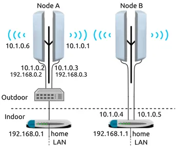
The OLSR topology can be biased by the choice of using multiple devices per super-node. We call a device an embedded system that includes at least a wireless and a wired interface. A super-node is composed of multiple devices connected to the same switch via the Ethernet interface.
Two example configurations of a super-node deserve to be described, in order to better understand the data collection
10.1.0.3 10.1.0.2 home LAN 10.1.0.1 192.168.0.1 Outdoor Indoor Node A home LAN 10.1.0.4 Node B 192.168.1.1 10.1.0.5 192.168.0.3 192.168.0.2 10.1.0.6
Figure A.16: Two example super-node configurations, each super-node is made of two devices.
phase. WCNs generally use two different addressing schemes for the mesh network and for the home LANs inside each user’s house. In Fig. A.16 we used 10.X.X.X/8 for the mesh network and the classes 192.168.X.X/24 for the home LANs. In the simplest case, each wireless and wired interface of a device in a super-node is assigned an IP address in the class 10.X.X.X, and wired interfaces also have an IP address in the 192.168.X.X class. Each device runs its own instance of the OLSR rout-ing protocol that manages both devices, makrout-ing it practically an independent node. The 192.168.X.X addresses are treated from OLSR as private networks, that is, the OLSR protocol is not running on those networks, but OLSR generates special sig-nalling packets to let each subnet reach the others. The wired interfaces are connected to a switch (normally placed directly in the rooftop) that is also connected to a device in the home of the user. This makes it easy to extend a super-node adding further devices since no change needs to be done on the existent ones. This configuration is used in node A in Fig. A.16.
Another configuration for super-nodes is to cable all the de-vices to the same router. The dede-vices are configured as stan-dard 802.11 APs/clients and do not run OLSR. The traffic coming from each device is isolated in the router using sep-arated VLANs terminated on virtual interfaces on the router which runs OLSR. This entirely masks the super-node structure from the network. This configuration, at the cost of increased configuration complexity, has two advantages: i) signalling is reduced since only the router runs OLSR, and ii) the original firmware can be left on the devices as long as it supports bridg-ing and VLAN taggbridg-ing. This configuration is used in Node B in Fig. A.16.
From a routing point of view, there is difference in the two configurations; in the first case, the super-node corresponds to two different IP addresses in the network, with a wired link con-necting them (thus, ETX will be fixed to 1). The resulting graph G(N, L) includes a clique of nodes with distinct IP addresses and edge weights constantly set to 1. In the second, each super-14
node corresponds to only one host (with two different IPs). We decided to merge super-nodes in one single logical node as this is functional to our analysis and also more representative of the network itself, for several reasons:
• The devices of a super-node all belong to the same person. If he is an attacker he will intercept traffic from all of them; • They are powered via the same source, connected to the same switch and they share the physical installation, so that failures due to physical damage, power outage or hu-man errors are correlated;
• Since the first configuration (Node A in Fig. A.16) of super-nodes is extremely inefficient, there are ongoing ef-forts to gradually migrate to the configuration with an ex-ternal router (Node B in Fig. A.16).
The process of merging super-node’s devices can not be ap-plied using only data from the OLSRd daemon. Further infor-mation must be gathered from distinct sources, and this pro-cess was aided by the participants to the communities. For the FFGraz network the naming style of each device is a domain-like convention in the form “phisical-interface.device.node”. This means that wifi0.device0.node0 and wifi1.device0.node0 are the first and second wireless interfaces of the first device of the same node. Every 10 minutes FFGraz publishes the topol-ogy using this naming convention. We are thus able to group the interfaces and the devices corresponding to the same node. FFWien instead exposes a JSON interface to the internal node database. The presence of a centralized node database is com-mon to many WCNs. It is used to com-monitor the evolution of the topology and to publish the network map on the commu-nity web server. Using the JSON interface we were able to map each IP address to each node, and compact the devices on the same node. For the FFWien network the data gathering process is split in two phases, one is the collection (every 5 minutes) of the OLSRd topology, and the second, once a day, is the access to the JSON interface to do node merging. The Ninux network currently does not expose a JSON interface but we had direct access to the node database updated every 5 minutes. Directly from the database we can access the topology, merge the nodes and collect the ETX values for each link.
Currently, we are not able to access information on the po-sition of nodes for all the networks. The interested reader can find maps of the physical topology on the website of the three networks8.
8See http://map.ninux.org/
https://karte.ffgraz.net/ https://map.funkfeuer.at/wien/