PhD thesis in Mathematical Models for Engineering,
Electromagnetism and Nanosciences
Carlo Alberini
Finite difference methods for
degenerate diffusion equations and
fractional diffusion equations
Advisor: Prof. Maria Agostina Vivaldi
Contents i
List of Figures v
List of Tables vii
Introduction ix
1 A nonlinear diffusion model for self-organized criticality phenomena 1
1.1 Preliminaries . . . 1
1.2 The Barbu’s continuous SOC model . . . 5
1.2.1 The nonlinear diffusion equation: existence and uniqueness of the solution . . . 6
1.2.2 The absorbtion of supercritical region into the critical one . . . 9
1.3 The Mosco’s fully discrete SOC model . . . 10
1.3.1 Discretization of time and space . . . 10
1.3.1.1 Time discretization . . . 10
1.3.1.2 Space discretization . . . 12
1.3.1.3 Construction of the forward difference gradient and the difference Laplacian . . . 14
1.3.2 The fully discrete SOC model . . . 19
1.3.3 Long-time behavior . . . 22
1.3.4 A priori estimate . . . 23
1.4 Numerical analysis . . . 25
1.4.1 The basic model . . . 25 i
1.4.2 Numerical approximations . . . 28
1.4.2.1 Fixed grid case . . . 28
1.4.2.2 Space-time synchronized grids case . . . 35
1.4.3 Numerical tests . . . 37
2 An Heaviside function driven degenerate diffusion model 45 2.1 The model . . . 46
2.1.1 Equivalence with the obstacle problem . . . 46
2.1.2 Asymptotic solution of the problem . . . 49
2.2 Numerical analysis . . . 54
2.2.1 Numerical approximation . . . 54
2.2.2 Numerical tests . . . 58
3 An Heaviside function driven degenerate diffusion model with Caputo time fractional derivative 65 3.1 The model . . . 65
3.1.1 Equivalence with the obstacle problem . . . 68
3.1.2 Asymptotic solution of the problem . . . 70
3.2 Numerical analysis . . . 72
3.2.1 Numerical approximation . . . 72
3.2.2 Numerical tests . . . 77
Conclusions and future developments 83 A Some theoretical aspects behind Chapter 2 - The obstacle problem 85 A.1 Preliminaries . . . 85
A.2 Main results . . . 89
B Some theoretical aspects behind Chapter 3 - Fractional calculus 91 B.1 Preliminaries . . . 92
B.2 Riemann-Liouville integrals . . . 97
B.3 Riemann-Liouville derivaties . . . 98
B.5 Caputo-Djrbashian derivative . . . 101 B.6 Bernstein functions . . . 103 B.7 A simple case . . . 104 B.7.1 Numerical approximation . . . 107 B.7.2 Numerical tests . . . 110 Acknowledgements 112 Bibliography 113 Bibliography 113
1.1 Example of the structure of the grid G0, G1 and G2. . . 13
1.2 Discret grids for m = 0, m = 1 and m = 2, i.e. G0, G1 and G2with the corresponding time ticking (in blue m parameter and in red s parameter).. . . 13
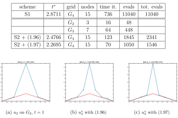
1.3 TEST 1. Initial datum (blue) and target function (red) . . . 38
1.4 TEST 1. Evolution of u, (S1) versus (S2) (η1, tol = 10−3, update (1.96)) . . . 39
1.5 TEST 1. Mk and Ek evolution with (S1) on G 4. . . 39
1.6 TEST 1. Scheme (S2): the update process after G2− G3refinement . . . 40
1.7 TEST 2. (in b) and c) the solution of (S1) is plotted every 45 iterations. . . 41
1.8 TEST 2. Solution evolution with scheme (S2) . . . 41
1.9 Test 3. Scheme (S1), u versus η . . . 42
1.10 TEST 3. Ek evolution . . . . 43
1.11 TEST 4. Solution evolution with (S1) on G3, times t = 1, 6, 9, 13 . . . 43
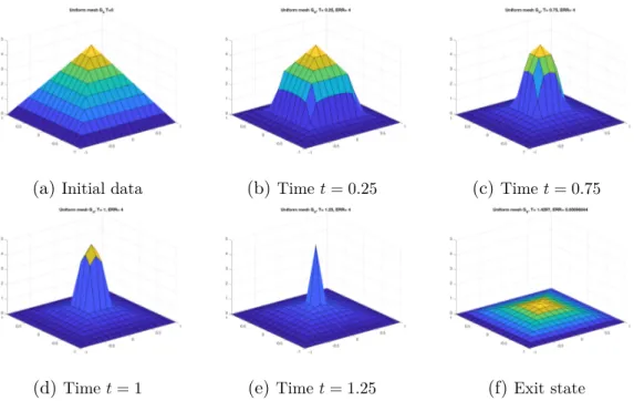
1.12 TEST 5. 2D-evolution of solution (scheme S1 on G4). . . 44
1.13 TEST 5. 2D-evolution of solution (scheme S2 on G2− G4) . . . 44
2.1 Graph of the functions uc(x), see 2.10, and u1(x), u2(x). . . . 50
2.2 Test 1. a) f = 0, b) discrete M (t) and I(t) evolution; c) f =−1.5. . . . 59
2.3 Test 1. Overestimation of the contact set for large γ: a) first time impact; b) final uncorrect solution. . . 59
2.4 Test 2. a) initial datum and final solution, b) t=0.05, c) t=0.09, d) discrete M (t) and I(t) evolution. . . . 61
2.5 Test 3. a) initial datum and final solution, b) t=0.04, c) t=0.08, d) t=0.16. . . 61
2.6 Test 4. a) f = 0, initial datum and final solution, b) M (t) and I(t) evolution, c) f =−4, d-e) f = 0 but initial datum close to the obstacle. . . . 62
2.7 a) Test 5, b) Test 6. . . 62
2.8 a) Test 7, b) Test 8, c) Test 9. . . 63
2.9 Test 10. a) f = 0, b) f =−2. . . . 64
3.1 Data of Example 1. . . 78
3.2 Solution for α = 0 and 128 no-des, scheme S3. . . . 81
3.3 Data of Example 2. . . 81
3.4 Example 2: polynomial error decay for α = 0.3, 0.6 and 0.9. . . . 82
B.1 The Mittag-Leffler fun-ction as a function of α. . . . 104
B.2 Solution at the midpoint as a function of α and the final time T = 1 (left) and T = 0.1 (right). . . 110
1.1 TEST 1. Performance comparison of schemes (S1) and (S2). . . 40
1.2 TEST 1. Stopping time t∗for different η functions on G4 when n grows. . . . 40
1.3 TEST 2. (η1, n = 10) Stopping time for (S1) versus a) tolerance, b) grid order. . . . . 42
2.1 Test 1. Performance comparison of scheme (S) with exact (H) or approximated (ηn)
Heaviside function, fixed (F) or variable (V) time step. . . 60
3.1 . . . 79
3.2 Example 2: N = 32, γα = 50, scheme S3. . . . 82
B.1 Relative error for the solution of the problem (B.7) for α = 0.5 and T = 1, in function
of N and M , scheme S1. . . . 111
B.2 Error for problem (B.7) for N = 32, T = 0.3, in function of α e γ, schemes S1 and S2.. 111
This thesis focuses on the study of three mathematical models consisting of degenerate diffusion equations and fractional diffusion equations arising from different study needs: the first one is taken from the study of self-organized criticality phenomena; the second one is connected to the obstacle problem, while the third one, that is a time-fractional type model, can find a wider use, for example, from biology to mechanics, to superslow diffusion in porous media, till financial type phenomena.
More precisely, in the first chapter of the present work, it will be described a numerical implementation of a differential model for the simulation of self-organized criticality (SOC) phenomena arising from recent papers by Barbu [11, 12], i.e.
ut− ∆H(u(t) − uc)∋ 0 in Ω × (0, ∞) u(0) = u0 > uc in Ω 0∈ H(u(t) − uc) on ∂Ω× (0, ∞) (1)
where Ω is a bounded subset of R2, uc ∈ C0(Ω) a given target function (called critical
state) and u0 a supercritical initial datum, while H is the multivalued Heaviside function:
H (r) = 1 if r > 0 [0, 1] for r = 0 0 if r < 0. (2)
We immediately state that the complete and appropriate conditions under which problem (1) is studied, through the aforementioned papers of Barbu, will be reported in the first chapter of the present work, together with a brief discussion that will be aimed
to showing the origins of the problem itself and its intrinsic mathematical structure, (see Sections 1.2 and 1.3).
However we can argue by saying that in that singular nonlinear diffusion problem the initial supercritical state evolves in a finite time towards the given critical solution, progressively from the boundary towards the internal regions. The key elements are the Heaviside function which plays the role of a switch for the dynamics, and the initial boundary contact with the critical state.
A finite difference implicit scheme on a fixed grid will be proposed in Section 1.4.2.1
for a regularized version of the problem, with the Heaviside replaced by a C1 function,
showing the same behavior of the solution: convergence in finite time toward the critical state on every single node, up to any prescribed accuracy, remaining supercritical during all the process, (related results will be presented in Section 1.4.1).
We will also implement this regularized version of the problem (1) through the use of synchronized spatial-temporal grids with progressive refinements (in the spirit of [46], see Section 1.4.2.2) simulates the appearance of short-range interactions of an increasing number of particles, speeding up the convergence to the critical solution and allowing a strong reduction of computational cost. The results of some numerical simulations are discussed in one and two dimensions, and they give the evidence that the temporal evolution of the solution u is characterized just by a progressive alignment to the target
function uc starting from the boundary of Ω, and proceeding towards the more internal
values.
Aim of the second chapter of the present work, instead, is to study the following problem:
ut− H (u − uc) (∆u + f ) = 0 a.e. in Ω, for all t∈ (0, T )
u (0) = u0 in Ω
u = 0 on ∂Ω, for all t∈ (0, T )
(3)
with T > 0, where H is the extended Heaviside function such that H(0) = 0, that is
H(r) = 1 for r > 0 0 for r≤ 0 (4)
and Ω is a bounded domain in Rn, n = 1, 2 with smooth boundary.
In this case, we will assume that the initial datum u0, the (independent of time) source
term f and the given target function (the obstacle) uc satisfy the following conditions
u0 ∈ H01(Ω) , f ∈ L2(Ω) , uc∈ H2(Ω) , uc≤ 0 on ∂Ω. (5)
and we will define as solution of problem (3) a function u ∈ L2(0, T ; H1
0(Ω)∩ H2(Ω)) ,
with ut∈ L2(0, T ; L2(Ω)) , which satisfies the equations in (3).
Under these assumptions and suitable conditions (see H1 and H2 explained in Section
2.1), we will able to show that the nonlinear degenerate parabolic problem (3), whose diffusion coefficient is now represented by the Heaviside function of the distance of the solution itself from a given target function, behaves as an evolutive variational inequality having the target as an obstacle: in other words, we will able to show that, under the aforementioned hypotheses, starting from an initial state above the target, the solution evolves in time towards an asymptotic solution, eventually getting in contact with part of the target itself. Finally, also for this model, through a finite difference approach, we will study the behavior of the solution of this problem, using in this case both the exact Heaviside function and a regular approximation of it, showing the results in some numerical tests, (see Section 2.2).
In the third chapter, at last, we will focus our attention on the following problem, which generalizes the one addressed in the second chapter, for 0 < α < 1:
∂α
tu− H (u − ψ) ∆u = 0 a.e. in Ω, for all t ∈ (0, T )
u (0) = u0 in Ω
u = 0 on ∂Ω, for all t∈ (0, T )
(6)
with T > 0, where H is, still, the extended Heaviside function (4) such that H(0) = 0
and Ω is a bounded domain in Rn, n = 1, 2 with smooth boundary. Only for simplicity,
we omitted in this case the presence of a forcing term in the problem.
Let us also precise that here ∂α
tu denotes the Caputo time-fractional derivative, that is, ∂tαu(x, t) := 1 Γ(1− α) ∫ t 0 (t− s)−α∂su(x, s) ds (7)
About the set of the assumptions adopted for this topic, we will define as solution of
problem (6) a function u∈ L2(0, T ; H1
0(Ω)∩ H2(Ω)) , with ∂tαu(x, t)∈ L2(0, T ; L2(Ω)) ,
which satisfies the equations in (6). Also for this model, it will be possible to prove the equivalence to the fractional parabolic obstacle problem, showing that its solution evolves
for any α ∈ (0, 1) to the same stationary state, the solution of the classic elliptic obstacle
problem. The only thing which changes with α is the convergence speed (see Section 3.1). Later, we will also study this problem from the numerical point of view, comparing some finite different approaches, and showing the results of some tests. We remark that these results extend what we will prove in the second chapter, that coincides with the case α = 1, (see Section 3.2.1).
We finally point out that the common feature of these three models lies in the different use made of the Heaviside (multi)function: in the formulation of evolutive differential problems is useful when a discontinuous behavior can occur according to the specific values of the solution itself: such a function acts as a dynamic switch for this behavior. It can be applied to the differential operator itself (for example, here, the Laplacian), giving rise to nonlocal phenomena: examples of that kind can be found in papers related to self-organized criticality such as the sandpile model (see e.g.[11, 12], [46], [47]). In these cases the Heaviside function, calculated on the distance between the solution and an assigned critical state, is able to govern the spread of the problem on a global level: the initial data tend to the critical state progressing from the edge towards the interior of the domain during the time evolution, which stops when all the solution gets in contact with the threshold critical state.
At last, referring to this particular behavior, it is interesting to note that the three typical aspects that we can find in general in every sandpile model, i.e. local equilibrium, threshold activation and diffusive character of the updating rules which cause the solution of (1) in the above settings to evolve in time towards the critical state, can be also shared by simple biological models of contamination and epidemic spreading, where the Heaviside term acts, also in this case, within the Laplace operator, as a switch of the process itself (see e.g. [37]).
Moreover, in the second example of use of the Heaviside function, i.e. as a degenerate diffusion coefficient applied externally to the Laplace operator, calculated between the
solution and the assigned critical state, it is able to locally control the diffusivity of the process in any areas where contact between solution and obstacle is reached.
Other examples of this approach can be found in the literature even without the Heaviside function, for example in cases where the model changes its behavior in a discontinuous way according to the values of the solution or of its partial derivatives: in these cases the Heaviside function could be replaced by the positive part function,
σ → (σ)+ := max{σ, 0}, for all σ ∈ R, to describe non-reversible phenomena that can be still connected to the avalanche behavior in the sandpile models [40] and to damage mechanics models [1].
A nonlinear diffusion model for
self-organized criticality phenomena
In this chapter, the basis theory behind SOC models will be analyzed, i.e. we will focus our attention above all those physical dynamic systems that spontaneously are able to rearrange themselves, in a finite time, from an any unstable configuration to a stable time-independent one, through the so-called avalanches phenomena.
In the meanwhile, we will also compare the two aforementioned scientific articles: the first one by V. Barbu (Self-organized criticality of cellular automata model; absorbtion in
finite-time of supercritical region into the critical one, (2013) Math. Methods Appl.
Sci.), [12] and the latter one by U. Mosco (Finite-time Self-Organized-Criticality on
syn-chronized infinite grids, (2018) SIAM J. Math. Anal., Vol. 50, No. 3), [46], since they
underlie, as said, some of the research results presented in the following Sections of this first chapter.
1.1
Preliminaries
A nice and suitable point of view for introducing the concepts described below could be to focus our attention on that part of real dynamic physical phenomena which have, among their main features, that of being dissipative. If analyzed in depth, a physical system of this kind tends to minimize its dissipations in order to stabilize itself around what it could be defined as a minimally stable state, rather than around other absolute stability criteria (like thermal equilibrium, for example).
This characteristic becomes extremely interesting to analyze when the physical sys-tem is composed of a large number of particles. In this case, in order to reach this minimally stable state, entire areas of the system can be observed, even experimentally, influencing each other thanks to the interactions due to the mutual presence of the par-ticles of the system itself. So, from this point of view, it is important to underlie that both the minimally stable state is continuously influenced by these (even minimal) per-turbations occurring between the particles in question and that these perper-turbations, even observed in nature, always occur at a short distance between the particles, but at a high frequency between them.
Finally, again for such physical systems, these continuous movements of particles generate what it is defined as avalanches, which tend to change their distribution over time within the physical system itself, until a stable configuration (i.e. the minimally stable state) is reached in a finite time. These avalanches of particles, during the temporal evolution of the system, can change their size in such a way as to dissipate the internal energy of the system, but, at the same time, prevent this dissipation from happening too
quickly. This dynamic continues until these avalanches end, and this happens when the
whole physical system has reached its (new) minimally stable state that, now, we can define as a critical state. Critical here means that this state is time-independent, but any (even minimal) perturbation of particles from this state moves the system toward another critical configuration through the production of other avalanches, but always in a finite time.
Typical examples of these physical systems are the mathematical models that describe the evolution of sandpiles over time. So, these models became the prototype for the study of many complex system dynamics where the current state evolves spontaneously towards a critical state in a finite time.
As mentioned above, the grains of sand (identifiable with the degrees of freedom of the system) of these models do not interact with each other at great distances, but are able to create avalanches of any size whenever, through the evolution of the system, a critical slope is reached locally within the sandpile itself.
It is interesting to note that the distribution of these avalanches within the sandpile follows a power law, while the character that emerges spontaneously from the evolution
mechanism of the system itself is called self-organized criticality (SOC below), given its peculiar characteristic of being able to rearrange itself in a time-dependet evolution that spontaneously brings it to a certain time-independet critical state. It is important to underlie that this evolution always last in a finite time. This critical state, that coincides with the minimally stable state defined above, can be thought as an attractor for all the dynamic. For a more detailed discussion, see [5, 6, 7] and [8].
The fundamentals of the SOC theory date back to the late 1980s, when Bak, Tang and Wiesenfeld [6, 7] introduced the sandpile cellular automata model in order to analyze
the time behavior of avalanches on a N × N plane lattice. In the model when the local
height hij of the sandpile at the ij-site reaches a prescribed critical threshold hc it
be-comes unstable, yielding the toppling of grains on the four adjacent sites. This automata dynamics was formalized by Dahr [27], who introduced the topplig matrix D: after a
toppling in the kℓ-site, the height hij of the sandpile at any site changes according to:
ht+1ij = htij − Dij,kℓ (1.1) where Dij,kℓ = 4 if ij = kℓ
−1 if ij and kℓ adjacent sites
0 otherwise.
(1.2)
By this rule subsequent topplings can occur, generating avalanches which end as soon
as stability is reached again over all the lattice sites (hij < hc at any site). In compact
form the toppling law can be interpreted as an implicit in time nonlinear finite difference system
ht+1− ht = DH(ht+1− hc) (1.3)
for the the vector of the heights h and the matrix D, and H is the standard Heaviside function:
H (r) = 1 if r≥ 0 0 if r < 0. (1.4)
Remark 1.1.1. The dynamic arising in (1.1) is directly connected to the equation (1.3)
that describes the only way to have a sand transfer to a site (activated) to another. In this last equation we have solution not equal to zero if and only if we are in the critical region, or above it, i.e. in the supercritical region. In all other cases the site it must be considered unchanged (stable).
Note that the matrix D recalls the well-known tridiagonal block matrix coming from the 5-point finite difference Laplacian approximation. It is henceforth not surprising that Carlson and Swindle [24] were able to characterize the continuum limit of the cellular automaton proposed by Bak, Tang and Wiesenfeld as the solution u(t) of the following singular diffusion equation
ut = ∆H(u(t)− uc) (1.5)
with uc a given critical state which plays the role of the threshold. Then the evolution
of the system toward the equilibrium can be described by two distinct time scales, a low one far from the critical state and a fast one in its neighborhood (corresponding to the avalanche process).
Due to the discontinuity of the Heaviside function, the ordinary existence results are not applyable to an equation as (1.5). That is why the multivalued setting was necessary to prove in general that the solution of such a problem exists and evolves spontaneously in
time towards the critical state ucfrom above; in other words, according to this assumption,
it will be possible to demonstrate that the supercritical region is absorbed into the critical one in a finite time, see [11, 12, 46].
Let us now introduce two articles on SOC phenomena, one by V. Barbu and one by U. Mosco, which represent the basis and starting point of this PhD thesis as well as some of the results produced. The articles are: Self-organized criticality of cellular automata
model; absorbtion in finite-time of supercritical region into the critical one (2013) by
grids (2018) by U. Mosco and they describe SOC models starting from very different
perspectives: the first one makes a continuous analysis of the phenomenon connecting the problem to the theory of semigroups in order to give existence, uniqueness and finite time absorption results, while the second proposes a totally discrete interpretation and analysis of the problem, however reaching similar results.
1.2
The Barbu’s continuous SOC model
Now, let’s start with the analysis of the article [12].
Let be u = u(x, t) the arbitrary state of the system and define it in a domain Ω⊂ Rn,
n = 1, 2, 3. Let us also consider the associated critical state uc = uc(x), x ∈ Ω, time-independent, and the following partition of the domain Ω
Ωt0 ={x ∈ Ω; u(x, t) = uc(x)} (critical region)
Ωt
− ={x ∈ Ω; u(x, t) < uc(x)} (subcritical region), and
Ωt
+ ={x ∈ Ω; u(x, t) > uc(x)} (supercritical region).
Let also the space of all Lebesgue measurable and p-integrable functions on Ω be
in-dicated with Lp(Ω), as 1≤ p ≤ ∞, and the corresponding norm with |·|
p. Moreover, let us
denote by Wk,p(Ω), Hk(Ω) = Wk,2(Ω), k = 1, 2, the standard Sobolev spaces on Ω, and let
us set H1
0(Ω) = {u ∈ H1(Ω); u = 0 on ∂Ω} and W
1,p
0 (Ω) = {u ∈ W1,p(Ω); u = 0 on ∂Ω},
where u = 0 on ∂Ω is taken in sense of traces.
Finally let us denote by H−1(Ω) the dual of H1
0(Ω) in the pairing⟨·, ·⟩ with the pivot
space L2(Ω). Moreover, let Y be a Banach space, it will be denoted with C([0, T ]; Y )
and Lp(0, T ; Y ) the spaces of Y−valued continuous, respectively Lp−integrable
func-tions, on [0, T ]. At last, let W1,p(0, T ; Y ) be the infinite dimensional Sobolev space
{ y ∈ Lp(0, T ; Y );dy dt ∈ L p(0, T ; Y ) } where dy
dt is given in the sense of vectorial
distri-butions. For more details, see [11] and [18].
In this setting, to well define the problem, the first important assumption to do in order to provide a continue analysis of the SOC model (1.5), since the equation holds
true for all i, j of the discrete square lattice N× N, is to substitute this finite discret 2-D
subset Ω⊂ Rn, and consider the generic point (i, j) as an element x in Ω, so to have the
previous model similar to the nonlinear diffusion equation (1.5) on the region Ω⊂ Rn in
the continuous time interval [0, T ].
Furthermore, the second important assumption, due to the discontinuity of the
stan-dard Heaviside function H, is to consider the multivalued Heaviside function eH which
enjoys the properties of maximal monotone graph inR × R (see [11]). This generalization
allows us to set the model (1.5) in a more general environment, invoking the theory of semigroups and coming to demonstrate results of existence, uniqueness and extinction of the SOC phenomenon in a finite time, so let us consider the following multivalued Heaviside function: e H(r) = 1 for r > 0 [0, 1] for r = 0 0 for r < 0. (1.6)
So, instead of equation (1.5), it will be considered the following multi-valued nonlinear diffusion problem: ∂u ∂t − ∆ eH (u (x, t)− u c (x))∋ 0 in Ω× (0, ∞) u (x, 0) = u0(x), x∈ Ω 0∈ eH (u (x, t)− uc(x)) x∈ ∂Ω and t ≥ 0. (1.7)
As shown in the following Section, it will be proved that the boundary value problem
(1.7) is well posed and the absorption of the supercritical region Ωt
+ of a sandpile into its
critical one Ωt
0 is reached in a finite time T not dependent of x, see [11, 12].
1.2.1
The nonlinear diffusion equation: existence and
unique-ness of the solution
In this Section it will be discussed the problem (1.7) by setting, for simplicity and without
any loss of generality, w (x, t) = u (x, t)− uc(x). So, the problem will be studied in the
∂w ∂t − ∆ eH(w (x, t))∋ 0 x∈ Ω, t > 0 w(0, x) = w0(x) x∈ Ω e H(w)∋ 0 on R+× ∂Ω (1.8)
with Ω bounded and open domain in Rn with smooth boundary ∂Ω, n≥ 1 and eH is the
multivalued Heaviside function (1.6).
The definition of the problem that it is now arising is concerned about the theory behind the porous media equation. It is known that for all equation of the form
∂w
∂t − ∆ψ(w) ∋ 0 (1.9)
with maximal monotone function ψ : R → 2R, the previuos problem (1.8) con be
re-written as an infinite dimensional Caucht problem in the space L1(Ω).
So, it is possible to get: dw dt + Aw(t)∋ 0 t > 0 w(0) = w0 (1.10)
where the operator A : D(A)⊂ L1(Ω)→ L1(Ω) is defined as:
Aw = { −∆η; η ∈ W1,1 0 (Ω), η(x)∈ eH(w(x)), a.e. x∈ Ω } . (1.11)
Following this definition, it holds that the domain of the operator A, D (A) is the set
of all w∈ L1(Ω) for which such a Section η ∈ W1,1
0 (Ω) of eH(w) exists.
In this case, it is possibile to proof that the operator A is also m−accretive in L1(Ω)
(see, [10], p.230); so, using the results of the classical Crandall - Liggett generation theorem
(see, [10], p.131) follow that for all w0 ∈ D(A) and T > 01, the infinite dimensional
Cauchy problem (1.10) has a unique mild solution w ∈ C ([0, T ]; L1(Ω)) expressed by:
w(t) = lim n→∞ ( I + t nA )−n w0, t≥ 0. (1.12)
Equivalently
w(t) = lim
ε→0wε(t) uniformly in t (1.13)
where wε denotes the step function
wε(t) = wεi for t∈ [iε, (i + 1)ε) (1.14)
where wiε is a solution of
wεi+1+ εAwi+1ε ∋ wiε, i = 0, 1, 2, . . . , N ; N =
[ T ε ] wε0 = w0. (1.15)
The main theorem in this Section is represented by the following result, that is concerned with the well-posedness of problem (1.8) , also given in (1.10) and (1.11) for-mulation:
Theorem 1.2.1. Assume that w0 ∈ L2(Ω). Then, (1.8) (or, more in general, the (1.10)
formulation) has a unique solution w satisfying
w∈ C([0, T ]; L1(Ω)∩ H−1(Ω))∩ W1,2(0, T ; H−1(Ω)), (1.16) dw dt (t)− ∆η(t) = 0, a.e. in Ω, t ∈ (0, T ) η(x, t)∈ eH(w(x, t)), a.e. (x, t)∈ Ω × (0, T ) (1.17) where η ∈ L2(0, T ; H1 0(Ω)). Moreover, t → ∫ Ω w(x, t)dx is absolutely continuous. If
w0 ∈ L∞(Ω), then w ∈ L∞(Ω× (0, T )). If w0 ≥ 0, a.e. in Ω, then w ≥ 0, a.e. in
Ω× (0, T ).
1.2.2
The absorbtion of supercritical region into the critical one
In this Section it will be set that u0, uc∈ L∞(Ω) and that u0(x)≥ uc(x), a.e. x ∈ Ω.
Then, by Theorem 1.2.1, for all T > 0, there is a unique evolution in time of the function u = u(x, t) satisfying problem (1.7) in the space (1.16). It means that
u∈ C ([0, T ]; L1(Ω)∩ H−1(Ω)) , du dt ∈ L 2(0, T ; H−1(Ω)) η ∈ eH (u− uc) , η∈ L2(0, T ; H1 0(Ω)) , u∈ L∞(Ω× (0, T )) u(x, t)≥ uc(x), a.e. (x, t) ∈ Ω × (0, T ) du dt − ∆η(t) = 0, a.e. in Ω, t ∈ (0, T ) u(0) = u0. (1.18)
Remark 1.2.1. It is posed that d
dt is the strong derivative of u in the strong topology of
H−1(Ω).
The main theorem in this Section is represented by the following result:
Theorem 1.2.2. Holding all of the previous assumptions, we have
u(x, t)− uc(x)≡ 0, a.e. x ∈ Ω, for all t ≥ T∗ (1.19)
where T∗ = p ∗ p∗− 2γ 2|y 0| 2 p∗ ∞ (∫ Ω y0dx )1−p∗2 . (1.20) Here, p∗ = 2d d− 2 for d ≥ 3, p
∗ > 2 for d = 1, 2 and γ is the Sobolev - Poincaré
inequality constant.
This means that, at time t = T∗, the supercritical region Ωt+ is completely absorbed into the critical zone Ωt0 and remains there for all t≥ T∗.
1.3
The Mosco’s fully discrete SOC model
Let us continue our analysis by introducing [46].
In this second paper, there are several new developed points about SOC models. In order to fully understand the point of view expressed in this work, and the deep reasons in it, it is important to keep in mind that the models that describe the behavior of sandpiles are a representation of intrinsically discrete natural physical dynamic systems, as they consist of a large number of interacting particles.
For this reason, starting from this assumption, the SOC mathematical model de-scribed in this Section is entirely discrete, and, due to this feature, it is able to take into account the short-distance and the high-frequency interaction between the particles of the system itself. We observe that this particular feature was lost in the previous model one,
as we passed from the discrete square lattice N × N to the continuous domain Ω ∈ Rn.
So, the novelty introduced in this article is just the presence of the numerical study of
the solution set in a discrete square lattice N×N, a priori infinite, domain whose number
of the initially considered points increases in a synchronized way following a progress in time according to geometric growth laws. For this reason we speak about the evolutionary process of the sandpile as an impulsive one, defined on an infinite space-time synchronized grid, and the model is fully-discret.
1.3.1
Discretization of time and space
Let us start to explain the adopted space-time synchronization over a discrete square
lattice N × N.
1.3.1.1 Time discretization
Let us start by discretizing time over the real half-line [0, +∞).
With the help of each multi-integer index
msℓk∈ (N ∪ {0})4
it is associated the time tℓ,k
tℓ,k m,s= 4m + 4−m(ℓ + k4−s) 0≤ m < +∞ 0≤ s < +∞ 0≤ ℓ ≤ 4m+1− 1 0≤ k ≤ 4s− 1 m, s, ℓ, k∈ N. (1.21)
Note that, for all s, the set of the indices mlk∈ (N ∪ {0})3 follows a lexicographical
order, as m, ℓ, k increase in their ranges. So, the immediate successive index that follows
msℓk is denoted by m′sl′k′. From this, two consecutive time instants
tℓ,km,s< tℓm′,k′,s′ are separated, on the positive real line, by quantity
tℓm′,k′,s′ − tℓ,km,s= 4−(m+s)
For given m and s, the set
Tm,s:= {
tℓ,km,s : 0≤ ℓ ≤ 4m+1− 1, 0 ≤ k ≤ 4s− 1} (1.22) divided into a partition the time interval [4m, 4 (m + 1)) into the subintervals
[
tℓ,km,s, tℓm,s′,k′
) . In accordance with the above, all of these subintervals have the same length, more precisely
equal to 4−(m+s). Moreover, it is introduced, for some m ≥ 0 and s ≥ 0 the following
notation
tLASTm,s := t4m,sm+1−1,4s−1 (1.23)
that simplify the recall of the last time instant in the corresponding subinterval, so it is
possible to say that tLAST
m,s = 4 (m + 1)− 4−(m+s). It is important to observe that tLASTm,s
converges to 4 (m + 1) from the left as s→ +∞. It is also set
T∞ := ∞ ∪ m=0 ∞ ∪ s=0 Tm,s. (1.24)
1.3.1.2 Space discretization
Let us consider a 2L diameter discrete square lattice N×N, where L > 0 is a given size
pa-rameter. It is defined also Ω = (−L, L)×(−L, L), ∂Ω = (−L × [−L, L])∪(L × [−L, L])∪
([− L, L ]× − L) ∪ ([ − L, L ]×L) and Ω = [−L, L] × [−L, L].
In this way it has been substituted the continuous set Ω, Ω and [0,∞) by the
core-spondent discrete grids of increasing cardinality.
Moreover, for every m ∈ N it has been defined the mesh size
hm = 2L
2m (1.25)
and set the discrete grids Gm ⊂ Ω, ∂Gm ⊂ ∂Ω, Gm ⊂ Ω as:
1. for m = 0, holds G0 =∅ and ∂G0 = G0 as the set of the 4 vertices of Ω, while
2. for m∈ N, holds Gm := {( q1 2L 2m, q2 2L 2m ) : (q1, q2)∈ Z2,|q1| ≤ 2m−1− 1, |q2| ≤ 2m−1− 1 } ∂Gm := {( q1 2L 2m, q2 2L 2m ) : (q1, q2)∈ Z2,|q1| = 2m−1,|q2| ≤ 2m−1− 1 } ∪ {( q1 2L 2m, q2 2L 2m ) : (q1, q2)∈ Z2,|q1| ≤ 2m−1− 1, |q2| = 2m−1 } ∪ {( q1 2L 2m, q2 2L 2m ) : (q1, q2)∈ Z2,|q1| = 2m−1,|q2| = 2m−1 } Gm := Gm∪ ∂Gm.
Thanks to these positions, Gm is composed of (2m− 1) × (2m− 1) distinct sites in
total, all in Ω while ∂Gm is composed of 2m4 sites in total, all on ∂Ω.
In the following it shall be considered
G∞ := ∞ ∪ m=0 Gm, ∂G∞:= ∞ ∪ m=0 ∂Gm, G∞:= G∞ ∪ ∂G∞ (1.26)
that are all countable space grids. It is set that G∞ ⊂ Ω, ∂G∞ ⊂ ∂Ω, G∞ ⊂ Ω. Figure
(1.1) shows the progressive refinement of the numerical grids Gm and the corresponding
growth of the number of the points inside them with the synchronized increase of the parameter m.
b
b
b
b
Discret grid for m = 0, i.e.
G0:= G0∪ ∂G0. b b b b b b b b b
Discret grid for m = 1, i.e.
G1:= G1∪ ∂G1. b b b b b b b b b b b b b b b b b b b b b b b b b
Discret grid for m = 2, i.e.
G2:= G2∪ ∂G2.
Figure 1.1: Example of the structure of the grid G0, G1and G2.
It is now clear as the space-time synchronization works: for all discrete grid Gm at a
mesh size given by hm we have a synchronized time interval of the type [4m, 4 (m + 1)).
As the parameter m increases, the mesh of the corresponding grid Gm grows and the time
ticking becomes correspondingly quicker.
1 2 3 4 5 6 7 8 9 10 11 12 t b b b b b b b b b b b b b b b b b b b b b b b b b b b b b b b b b b b b b b b b b b b b b b b b b b b b b b b b b b b b b b b b b b b b b b b b b b b b b b b b b b b b b b b b b b r r r r r r r r r r r r r r r r rrrrrrrrr rr rrrrrrrrrrrrrrrrrrrrrrrrrrrrrrrrrrrrrrrrrrrrrrrrrrrrr rr r r r r r r r r r r r r r r r r r r r r r r r r r r r r r r r r r r r r r r r r r r r r r r r r r r r r r r r r r r r r r r rrrrrrrrr rr rrrrrrrrrrrrrrrrrrrrrrrrrrrrrrrrrrrrrrrrrrrrrrrrrrrrr
Figure 1.2: Discret grids for m = 0, m = 1 and m = 2, i.e. G0, G1and G2with the corresponding time
A more simple notation is now introduced for grid sites and functions set on them:
for every fixed m∈ N, it holds in an equivalent way that
ij = (ihm, jhm) = (q1hm, q2hm)∈ Gm
and for every function u on Gm,
uij = u (ihm, jhm) = u (q1hm, q2hm) .
1.3.1.3 Construction of the forward difference gradient and the difference Laplacian
With this notation, for a function u defined on Gm it shall be set the forward difference
x1-partial derivative ( D+1mu)ij = 1 hm [ u(i+1)hm,jhm− uihm,jhm ] = 1 hm [ui+1j− uij] (1.27)
at the sites ij = (q1hm, q2hm)∈ Gm with − 2m−1 ≤ q1 ≤ 2m−1− 1 and − 2m−1 ≤ q2 ≤
2m−1, the forward difference x
2-partial derivative ( D+2mu)ij = 1 hm [u (ihm, (j + 1)hm)− u (ihm, jhm)] = 1 hm [uij+1 − uij] (1.28)
at the sites ij = (q1hm, q2hm)∈ Gm with−2m−1 ≤ q1 ≤ 2m−1 and−2m−1 ≤ q2 ≤ 2m−1−1,
the forward difference gradient ( ∇+ mu ) ij = (( D+1mu)ij,(D+2mu)ij ) (1.29)
at the sites ij = (q1hm, q2hm) ∈ Gm with −2m−1 ≤ q1 ≤ 2m−1 − 1 and −2m−1 ≤ q2 ≤
2m−1− 1.
Now, for every function u on Gm and at every site ij ∈ Gm, it is set the centered
difference Laplacian ∆m, as
(∆mu)ij =
1
h2 m
[4uij− ui−1j− ui+1j− uij−1− uij+1] ∀ij ∈ Gm. (1.30) Moreover, in the following, it will be useful the next equality that holds for every
N ∑ k=0 (ak+1− ak) (bk+1− bk) = = (aN +1− aN) bN +1− (a1− a0) b0+ ∑N k=1(2ak− ak−1− ak+1) bk. (1.31)
From (1.31) and by considering ak = ukjand bk= vkj, for−2m−1≤ k = q1 ≤ 2m−1−1
and for every fixed j with −2m−1 ≤ j = q
2 ≤ 2m−1, it follows that 2m∑−1−1 k=−2m−1 (uk+1j − ukj) (vk+1j− vkj) = =(u2m−1j− u(2m−1−1)j)v2m−1j −(u(−2m−1+1)j − u(−2m−1)j)v(−2m−1)j+ + 2m∑−1−1 k=−2m−1+1 ( 2ukj − u(k−1)j− u(k+1)j ) vkj.
Moreover, if holds that v = 0 on ∂Gm, the previous inequality becomes
2m∑−1−1 k=−2m−1 (uk+1j − ukj) (vk+1j − vkj) = 2m∑−1−1 k=−2m−1+1 ( 2ukj − u(k−1)j− u(k+1)j ) vkj (1.32)
considering the definition of D+1m (1.27), the equality (1.32) reduces to
2m−1∑−1 k=−2m−1 ( D1m+ u)kj(D+1mv)kj = 2m−1∑−1 k=−2m−1+1 1 h2 m ( 2ukj − u(k−1)j− u(k+1)j ) vkj. (1.33)
On the other hand, by summing both sides of (1.33) over−2m−1 ≤ j = q2 ≤ 2m−1−1
and noting that the right-hand side vkj = 0 for j = −2m−1 for every k, it is possible to
write the identity
2m∑−1−1 j=−2m−1 2m∑−1−1 k=−2m−1 ( D+1mu)kj(D+1mv)kj = 2m−1∑−1 j=−2m−1−1 2m−1∑−1 k=−2m−1+1 1 h2 m ( 2ukj− u(k−1)j − u(k+1)j ) vkj (1.34)
for all functions u and v on Gm with v = 0 on ∂Gm.
Similarly, for all functions u and v on Gm with v = 0 on ∂Gm, holds
2m−1∑−1 k=−2m−1 2m−1∑−1 j=−2m−1 ( D2m+ u)kj(D2m+ v)kj = 2m∑−1−1 k=−2m−1+1 2m∑−1−1 j=−2m−1+1 1 h2 m ( 2ukj − uk(j−1)− uk(j+1) ) vkj. (1.35)
Working with (1.34) and (1.35) together, it is possible to have the identity
2m∑−1−1 i,j=−2m−1 [( D+1mu)ij(D+1mv)ij +(D+2mu)ij(D2m+ v)ij ] = ∑ ij∈Gm (∆mu)ijvij (1.36)
that, as said before, is satisfied by all functions u = (uij) and v = (vij) on Gm with vij = 0
for every ij ∈ ∂Gm, where ∆mu = (∆mu)ij∈Gmis the centered difference Laplacian defined
in (1.30).
All the above defined tools find their natural mathematical collocation in the following
Hilbert space, more precisely: for every m∈ N it is set
Ym = {
u = (uij) : ij ∈ Gm }
(1.37) with inner product
⟨u, v⟩m = ∑
ij∈Gm
uijvijh2m, u = (uij)∈ Ym, v = (vij)∈ Ym (1.38)
and norm
∥u∥m =⟨u, u⟩1/2m . (1.39)
Then, for vectors ∇+
mu = ( D+1mu, D2m+ u) and ∇+ mv = ( D1m+ v, D2m+ v), holds
⟨∇+ mu,∇+mv⟩m = ⟨ D1m+ u, D1m+ v⟩ m+ ⟨ D+2mu, D+2mv⟩ m with ⟨ D1m+ u, D+1mv⟩m =∑2i,j=m−1−2−1m−1 ( D1m+ u)ij(D+1mv)ijh2 m ⟨ D2m+ u, D+2mv⟩m =∑2i,j=m−1−2−1m−1 ( D2m+ u)ij(D+2mv)ijh2 m (1.40) and sets ∇+ mu m = ⟨ ∇+ mu,∇ + mu ⟩1/2 m .
In this Hilbert-space, it is possible to write the identity (1.36) in the following way ⟨ ∇+ mu,∇ + mv ⟩ m =⟨∆mu, v⟩m (1.41)
u = (uij) and v = (vij) on Gm with vij = 0 for every ij ∈ ∂Gm.
Remark 1.3.1. It is important to point out that ∆mu = (∆mu)ij∈Gm is the centered
difference Laplacian defined in (1.30).
Now, it has been introduced the following subspace:
Xm ={u = (uij)∈ Ym : uij = 0 ∀ij ∈ ∂Gm} (1.42)
of Ym. This space is a Hilbert on itself and it is endowed with the following inner product
(u, v)m =⟨u, v⟩m+ ⟨ ∇+ mu,∇ + mv ⟩ m, u = (uij)∈ Ym, v = (vij)∈ Ym. (1.43)
Moreover, in this contest it is possible to prove that on Xm holds the following discrete
Poicaré inequality
∥u∥m ≤ cP ∇+u m ∀u ∈ Xm (1.44)
with cP = L
√
2 .
To give existence and uniqueness results, it will be now built an equation (see (1.47)) that has the required features. In order to do this, it is now introduced on the subspace
Xm of Ym the bilinear form Em(u, v) = ⟨∇m+u,∇+mv⟩m with ⟨∇
+
mu,∇+mv⟩m is given by
Em(u, v) =⟨∇+mu,∇+mv⟩m = = 2m∑−1−1 i,j=−2m−1 [( D1m+ u) ij ( D1m+ v) ij + ( D2m+ u) ij ( D+2mv) ij ] h2m (1.45)
in the domain D [Em] = Xm. By (1.44), it is possible to assert that the form Em(u, v) is
coercive
1
c2
P + 1
(u, u)2m ≤ Em(u, u) ∀u ∈ Xm (1.46)
and that the inner product (u, v)m, set in (1.42), is equivalent to the form Em(u, v). For
every m∈ N ∪ {0}, it is now defined the linear operator
Gm : Ym 7→ Ym
as follows. For every f ∈ Ym it is set u = Gmf as the solution of
u∈ Xm : Em(u, v) =⟨f, v⟩m ∀v ∈ Xm (1.47)
Moreover, using (1.46), for every f ∈ Ym is possible to say that the solution u of
(1.47) exists and is unique. For a more detailed discussion, see [46], pp. 2414 – 2417.
The most important point of this Subsection is that the operatorGm and the centered
difference Laplacian ∆mu = (∆mu)ij∈Gm, previously defined in (1.30), are related on Xm
by the identity
Gm(∆mu) = u (1.48)
and that it is satisfied componentwise the relation
(Gm(∆mu))ij = uij ∀ij ∈ Gm (1.49)
for every u = (uij)ij∈Gm, u∈ Xm.
Now, to conclude this preparation of the discrete Mosco model for sandpiles, associ-ated with the multivalued Heaviside function
e H(r) = 1 for r > 0 [0, 1] for r = 0 0 for r < 0 (1.50)
it is introduced another operator, namely
H : Ym7→ Ym (1.51)
in Ym through the relation η ∈ H(z) for generic vector functions z ∈ Ym, z = (zij)ij∈Gm,
η∈ Ym, η = (ηij)ij∈Gm componentwise as
(H(z))ij = H (zij) ∀ij ∈ Gm (1.52)
i.e.,
ηij = 0 if zij < 0; 0≤ ηij ≤ 1 if zij = 0; ηij = 1 if zij > 0 ∀ij ∈ Gm.
This multivalued operator z→ H(z) is
1. monotone in Xm× Xm because it satisfies (see [10], p.43)
⟨η1− η2, z1− z2⟩m ≥ 0 ∀ηi ∈ H (zi) , zi, ηi ∈ Xm, i = 1, 2 (1.53)
2. maximal monotone and coercive because the range of z → λz + H(z) is all of Xm
for every λ > 0.
By this features it can be said that Gm + cH is maximal monotone and coercive
on Xm × Xm for every constant c > 0 and its range is all of Xm. For a more detailed
discussion, see [46], p. 2417. This is the fundamental condition to have the existence proof of the following results.
1.3.2
The fully discrete SOC model
We are now ready to introduce the fully discret Mosco SOC model. The model is set on
Remark 1.3.2. For a function u set in G∞, the restriction of u to Gm is could be denoted
by um.
In this model, the given data are (given) functions uc = (uc
ij )
ij∈G∞ (the meaning of
these functions is to be the sandpile critical state) and u0 =(u0
ij )
ij∈G∞ (this is, instead,
the sandpile initial configuration).
Both functions are defined on G∞ and satisfy the following conditions
uc=(uc ij ) ij∈G∞, u 0 =(u0 ij ) ij∈G∞ satisfying u0 ij ≥ ucij ∀ij ∈ G∞, u0ij = ucij ∀ij ∈ ∂G∞. (1.54)
That is, the model is based on two sets of equations:
1. the first set of equations define the solutions u(s)(tℓ,k
m,s ) for (tℓ,k m,s, ij ) ∈ Tm,s× Gm.
(a) For fixed ms ∈ N × N, they are iteratively get in ℓ, k by the following
finite-difference scheme with given initial conditions u∗m on the grid Gm
u(s)(t0,0 m,s ) = u∗m on Gm u(s)(tℓ′,k′ m,s ) = u(s)(tℓ,k m,s ) − 4−(m+s)∆ m ( ηℓ′,k′ m,s ) with ηm,sℓ′,k′ ∈ H(u(s)(tm,sℓ′,k′)− ucm) on Gm u(s)(tℓm,s′,k′) = u(s)(tm,sℓ,k )= ucm, ηℓm,s′,k′ = 0 on ∂Gm (1.55)
for 0 ≤ ℓ < 4m+1 − 1, 0 ≤ k ≤ 4s − 1. We note that the index ℓ′, k′ is the
index-pair successive to ℓ, k in the lexicographic order. The times t0,0m,s are
independent of s; in fact, it holds that t0,0
m,s= 4m for all s.
2. the second set of equations is determined iteratively in m∈ N∪{0} and it is referred
to the sequence of initial states u∗m on the grids Gm in the preceding equations.
(a) For m = 0, u∗m = u∗0 is assigned by setting
(b) while, for given indices 1 ≤ m ≤ n, n ∈ N, u∗m is given on the grid Gm in three levels:
i. for every s∈ {N}, it is set that
u∗m(ij) = uc(ij) + 4 ( u(s)m−1 ( t4mm−1,s−1,4s−1, ij ) − uc(ij)) ∀n ≥ 1, ∀1 ≤ m ≤ n, ∀ij ∈ Gm∩ Gm−1 = Gm−1, (1.57)
ii. then, it is also set
u∗m(ij) := uc(ij) +1
44−(n−m)(u
0(ij)− uc(ij))
∀n ≥ 1, ∀1 ≤ m ≤ n, ∀ij ∈ Gm− Gm−1,
(1.58)
iii. in the end, it is defined
u∗m(ij) = uc(ij) ∀ij ∈ ∂Gm. (1.59)
In these three steps it has been defined the complete calculation of u∗m on
the grids Gm, Gm = Gm∪ ∂Gm, for all m, here considered.
Remark 1.3.3. Note that for m = 0, G0 = ∂G0 ={ij : i, j = ±2m} consists of the
4 vertices of the square [−L, L] × [−L, L]. Moreover, u00 = uc0 on G0.
Remark 1.3.4. The value u(s)m−1
(
t4mm−1,s−1,4s−1, ij
)
= u(s)m−1(tLASTm,s ) is the last value got by the solution on the grid G at the step m− 1 in the time interval [t0,0m−1, tm
)
.
Now, we give the most relevant result in this Section:
Theorem 1.3.1. We are given an initial state u0 and a critical state uc on G∞ satisfying
(1.54). We fix an arbitrary s ∈ N. Then for all m ∈ N, all 0 ≤ ℓ ≤ 4m+1 − 1, and all
0≤ k ≤ 4s−1 and for all discrete times tℓ,km,s≥ 0 as in (1.21), there exists a unique solution
u(s), with values u(s)(tℓ,k m,s
)
, of the impulsive system from (1.55) to (1.59). Moreover,
where
Mm := max
ij∈Gm
{
u0ij − ucij}. (1.61)
Theorem and proof can be found in [46], pp. 2425–2436.
Remark 1.3.5. Analyzing the result of Theorem 1.3.1, which is given for a fixed grid
Gm and a given time set [4m, 4 (m + 1)), it is possible to say that it does not get any
information about the long-time behavior of the solutions. To give some information about it, it is necessary fix additional hypothesis on the data.
1.3.3
Long-time behavior
This Section is based on the study of the discrete model considered in Theorem 1.3.1. The
basic data of this model are two real-valued functions u0 (initial sandpile state) and uc
(critical sandpile state) pointwise defined on G∞ introduced in (1.26). For the following
results, it shall be assumed that condition (1.54) holds and that there exist two constant
M∞ and M1 s.t. 0 < M∞ < +∞, M1 < +∞ (1.62) defined as M∞:= M∞(u0− uc)= sup ij∈G∞ ( u0(ij)− uc(ij)), (1.63) M1 := M1 ( u0− uc)= sup n∈N ∑ ij∈Gn ( u0(ij)− uc(ij))h2n. (1.64) For τ = 4m + ℓ4−m, m≥ 0, ℓ ∈ {0, . . . , 4m+1− 1}, it is set Φ∞(τ ) := lim inf s→+∞ ∑ ij∈Gm ( u(s)(tℓ,km,s, ij)− (uc)ij ) h2m (1.65) where u(s)(tℓ,k m,s )
are the solutions of the impulsive system from (1.55) to (1.59). It is also set
T∗ := sup{4n : n ∈ N, such that Φ∞(τ ) > 0 ∀0 ≤ m ≤ n
∀τ ∈ [4m, 4(m + 1)), τ = 4m + ℓ4−m, ℓ ∈ {0, . . . , 4m+1 − 1}} ∈ [0, +∞]
(1.66)
This Section is concluded by the following theorem:
Theorem 1.3.2. Let u0 and ucbe two functions defined on the infinite grid G
∞, satisfying
the assumptions (1.54) and (1.62). Then, there exist a grid Gm∗ and a finite time τ∗ = 4m∗+ ℓ∗4−m∗, m∗ ≥ 0, 0 ≤ ℓ∗ ≤ 4m∗+1− 1, such that the solutions u(s) of the system from (1.55) to (1.59) satisfy the property
Φ∞(τ∗) = 0 (1.67)
implying
T∗ < +∞. (1.68)
Theorem and proof can be found in [46], pp. 2436–2437.
1.3.4
A priori estimate
In this last Section, by strengthening the assumptions on the data functions u0 and uc,
it will be given a more precise and explicit estimate about the finite equilibrium time T∗
with a direct connection and dependence by the initial data.
About the following Section it shall be considered a coarses time grid. For every
m∈ N and ℓ = 0, . . . , 4m− 1 hold the times
tℓm = 4m + ℓ4−m (1.69)
The set
Tm := {
tℓm : 0≤ ℓ ≤ 4m+1− 1} (1.70)
T∞:= n ∪ m=1
Tm. (1.71)
For τ ∈ T∞, there are a unique m ∈ N ∪ {0} and a unique ℓ ∈ {0, . . . , 4m− 1}, s.t.
τ = tℓ m ∈ Tm. At last, we define Φ∞(τ ) := lim sup s→+∞ ∑ ij∈Gm ( u(s)(tℓ,km,s, ij)− (uc)ij ) h2m (1.72)
where us= u(s)(tℓ,km,s) are the solutions of the impulsive system from (1.55) to (1.59) .
Theorem 1.3.3. Let u0 and uc be the restrictions to G∞ of two continuous functions u0 ≥ uc on Ω such that u0− uc is Lipschitz continuous on Ω Then, we have
Φ∞(τ ) = 0 (1.73)
for all τ ∈ T∞, τ ≥ τ∗, where
τ∗ := A−2 [( |B| 4 )1 2 + ( C 4 )1 2 ]2 < +∞. (1.74)
The constants in (1.74) are defined as follows:
A := 2CS−2M−
1 2
∞ (1.75)
where M∞ = M∞(u0− uc) is given by (1.63) and C
S is a constant depending only on L
and p; B := ∫∫ O ( u0− uc)dxdy (1.76) C := CLip2L √ 2 (1.77) where CLip = CLip ( u0 − uc) (1.78)
is the Lipschitz seminorm of u0− uc on Ω.
1.4
Numerical analysis
This Section is devoted to a numerical study of the evolutionary non singular problem (1.7) as presented in [12] through an implicit finite difference approach. As to do so, in a similar way to what is in (1.3) done, we have to replace the multivalued Heaviside function with a smooth approximation of it: this will be discussed in Subsection 1.4.1, together with some properties of this regularized problem.
The numerical scheme is implemented in Subsection 1.4.2.1 on a fixed space grid. Since the discrete settings cannot reproduce completely the fine spatial interactions of the continuous model, the finite time convergence corresponds to the time evolution of the numerical solution to the target on every single node up to any prescribed accuracy, globally with exponential rate, remaining supercritical during all the process.
In Subsection 1.4.2.2 we will adapt our scheme to a space-time synchronized family of grids in order to reduce the convergence time and the total computational cost. The idea, as said, is inspired by the recent paper of Mosco [46], above discussed, where a fully discrete analytic model allowing for infinite degrees of freedom is studied to preserve the physical aspect of SOC phenomena which are intrinsically discrete particle processes, better captured by discrete equations on an infinite spatial-temporal lattice incorporating arbitrary short-range and high-frequency particle interactions. The equations of the pro-cess on each finite spatial grid are coupled in time with an impulsive change of the initial data at each refinement, keeping constant the parabolic ratio between the discretization steps, up to the desired accuracy.
In Subsection 1.4.3 we finally present the results of some numerical simulations both in one and two dimensions.
1.4.1
The basic model
In view of the discretization of problem (1.7), we first of all introduce a regular
approx-imation η ∈ C1(R) of H in a neighborhood of the origin, for example by means of the
η1(r) = 1 if r > 1 n −n3r3 4 + 3 4nr + 1 2 if − 1 n ≤ r ≤ 1 n 0 if r <−1 n. (1.79)
With respect to the integer parameter n∈ N, we see that η1(r) = eH(r) for |r| ≥
1 n, and that eH− η1 L1(−1,1)= ∫ 1 −1| e H(r)− η1(r)| dr = ∫ 1/n −1/n| e H(r)− η1(r)| dr → 0 as n → ∞. (1.80)
Note that η1(0) = 0.5, so that this will be the value taken at the contact points
between the solution of problem (1.7) (with eH replaced by η1) and the critical one,
in particular at the boundary. Moreover, the values of η1 in (0.5, 1] characterize the
supercritical states of the solution, those in [0, 0.5) the subcritical ones.
There are of course other possible candidates for the approximation of eH. For
exam-ple the following monotone functions
η2(r) = 1 (1 + e−nr) , or η3(r) = 1 2+ 1 πarctan(nr) (1.81)
have similar properties for a large n, even if in those cases the support of ( eH− η) is
un-bounded. The numerical tests show that the choice of η slightly influences the qualitative behavior of the solution, that is the way it converges to the target (more impulsive for
η1, more smooth for the other choices), but it is not relevant for the final time of
conver-gence, which is essentially determined by the quantity η′(0) (in the previous examples:
η′1(0) = 3n/4, η2′(0) = n/4, η3′(0) = n/π): the higher is this value, the closer we are to
the real Heaviside, and the faster is the convergence to the target (see Section 1.4.3). The problem to solve then becomes:
ut− ∆η(u − uc) = 0 in Ω× (0, ∞) u(0) = u0 > uc in Ω u = uc on ∂Ω× [0, ∞), (1.82)
where η denotes one of the approximate Heaviside functions previously defined, for a fixed large parameter n that for simplicity from now on we neglect.
If we set w (x, t) := u (x, t)− uc(x), problem (1.82) can also be written as: wt− ∆η(w) = 0 in Ω × (0, ∞) w(0) = w0 > 0 in Ω w = 0 on ∂Ω× [0, ∞). (1.83)
Applying the divergence theorem, together with the boundary conditions on w, we get: ∫ Ω ∆η (w) dx = I ∂Ω ∇η (w) · ⃗n ds = I ∂Ω η′(w)∇w · ⃗n ds = η′(0) I ∂Ω ∂w ∂n ds≤ 0, (1.84)
since η′(0) > 0 (η is increasing at the origin) and the normal derivative of w on the
boundary in the direction of the external normal vector is non positive. From (1.83) and (1.84) then follows:
∫ Ω wt dx = ∫ Ω ∆η (w) dx≤ 0 (1.85)
according to that, if we define the two quantities:
M (t) = ∫ Ω w(x, t) dx, E(t) =− ∫ Ω ∆η(w) dx (1.86)
then we have M′(t)≤ 0 and E(t) ≥ 0.
In other words, from (1.86), M (t), which can be interpreted as the total mass of the problem (that is the global distance from the target), always decreases with time. This fact does not imply that w decreases at any point of Ω: from (1.83) we see that this should be equivalent to say that the function η(w) be globally superharmonic in Ω. Of course, according to the specific given initial data, this could not be the starting situation. In fact the second quantity E(t), which represents a sort of distance from harmonicity for
η(w), might initially grow before it starts to decrease toward zero. We will find the same
behavior even in the discrete settings.
For the original continuous model (1.7) it was proved in [12] that u(t) → uc (and
M (t) → 0) in finite time. Asimptotically, model (1.82) shares the same properties. In
particular at any point of Ω as t grows: w(t)→ 0, η(w(t)) → 0.5, and ∆η(w(t)) → 0. We
will prove these properties for the finite difference solution of an implicit scheme which discretizes (1.82).