On the Chemical Abundances of Miras in Clusters:
V1 in the Metal-rich Globular NGC 5927
*V. D’Orazi1,2 , D. Magurno3,4, G. Bono3,4 , N. Matsunaga5,6, V. F. Braga7,8 , S. S. Elgueta5, K. Fukue6, S. Hamano6, L. Inno9, N. Kobayashi6,10, S. Kondo6, M. Monelli11 , M. Nonino12, N. Przybilla13, H. Sameshima6, I. Saviane14, D. Taniguchi5, F. Thevenin15, M. Urbaneja-Perez13, A. Watase16, A. Arai6, M. Bergemann9 , R. Buonanno3,17, M. Dall’Ora18 , R. Da Silva4,19,
M. Fabrizio4,19 , I. Ferraro4, G. Fiorentino20 , P. Francois21, R. Gilmozzi14, G. Iannicola4, Y. Ikeda6,22 , M. Jian5 , H. Kawakita6,23, R. P. Kudritzki24, B. Lemasle25, M. Marengo26 , S. Marinoni4,19, C. E. Martínez-Vázquez27, D. Minniti7,8,
J. Neeley28 , S. Otsubo16, J. L. Prieto7,29 , B. Proxauf30, M. Romaniello14, N. Sanna31, C. Sneden32 , K. Takenaka16, T. Tsujimoto33 , E. Valenti14 , C. Yasui33, T. Yoshikawa34, and M. Zoccali7,35
1
INAF Osservatorio Astronomico di Padova, vicolo dell’Osservatorio 5, I-35122 Padova, Italy;[email protected]
2
Monash Centre for Astrophysics, School of Physics and Astronomy, Monash University, Melbourne, VIC 3800, Australia 3
University of Roma Tor Vergata, via della Ricerca Scientifica 1, I-00133 Roma, Italy 4
INAF Osservatorio Astronomico di Roma, via Frascati 33, I-00040 Monte Porzio Catone RM, Italy 5
Department of Astronomy, The University of Tokyo, 7-3-1 Hongo, Bunkyo-ku, Tokyo 113-0033, Japan 6
Laboratory of infrared High-resolution spectroscopy(LiH), Koyama Astronomical Observatory, Kyoto-Sangyo University, Motoyama, Kamigamo, Kita-ku, Kyoto 606-8555, Japan
7Instituto Milenio de Astrofisica, Av. Vicuña Mackenna 4860, 782-0436 Macul, Santiago, Chile 8
Departamento de Fisica, Facultad de Ciencias Exactas, Universidad Andres Bello, Av. Fernandez Concha 700, Las Condes, Santiago, Chile 9
Max-Planck Institute for Astronomy, D-69117 Heidelberg, Germany 10
Kiso Observatory, Institute of Astronomy, The University of Tokyo, 10762-30 Mitake, Kiso-machi, Kiso-gun, Nagano 397-0101, Japan 11
Instituto de Astrofsica de Canarias, Calle Via Lactea s/n, E-38205 La Laguna, Tenerife, Spain 12
INAF Osservatorio Astronomico di Trieste, Via G.B. Tiepolo 11, I-34143 Trieste, Italy 13
Institut für Astro- und Teilchenphysik, Universität Innsbruck, Technikerstrasse 25, A-6020 Innsbruck, Austria 14
European Southern Observatory, Karl-Schwarzschild-Str. 2, D-85748 Garching bei München, Germany 15
Université de La Côte d’Azur, OCA, Laboratoire Lagrange CNRS, BP. 4229, F-06304 Nice Cedex, France 16Division of Science, Graduate School, Kyoto Sangyo University, Motoyama, Kamigamo, Kita-ku, Kyoto 606-8555, Japan
17
INAF Osservatorio Astronomico d’Abruzzo, Via Mentore Maggini snc, Loc. Collurania, I-64100 Teramo, Italy 18
INAF Osservatorio Astronomico di Capodimonte, Salita Moiariello 16, I-80131 Napoli, Italy 19
SSDC, via del Politecnico snc, I-00133 Roma, Italy 20
INAF Osservatorio Astronomico di Bologna, Via Ranzani 1, I-40127 Bologna, Italy 21
Observatoire de Paris, PSL Research University, CNRS, Place Jules Janssen, F-92190 Meudon, France 22
Photocoding, 460-102 Iwakura-Nakamachi, Sakyo-ku, Kyoto 606-0025, Japan 23
Department of Astrophysics and Atmospheric Sciences, Faculty of Science, Kyoto Sangyo University, Motoyama, Kamigamo, Kita-ku, Kyoto 603-8555, Japan 24
Institute for Astronomy, University of Hawaii, 2680 Woodlawn Drive, Honolulu, HI 96822, USA 25
Astronomisches Rechen-Institut, Zentrum für Astronomie der Universität Heidelberg, Mönchhofstr. 12-14, D-69120 Heidelberg, Germany 26
Department of Physics and Astronomy, Iowa State University, Ames, IA 50011, USA
27Cerro Tololo Inter-American Observatory, National Optical Astronomy Observatory, Casilla 603, La Serena, Chile 28
University of Florida, Department of Astronomy, 211 Bryant Space Science Center, P.O. 112055, Gainesville, FL, USA 29
Núcleo de Astronomía, Facultad de Ingeniería y Ciencias, Universidad Diego Portales, Ejército 441, Santiago, Chile 30
Max Planck Institute for Solar System Research Justus-von-Liebig-Weg 3, D-37077 Göttingen, Germany 31
INAF Osservatorio Astronomico di Arcetri, Largo Enrico Fermi 5, I-50125 Firenze, Italy 32
Department of Astronomy C1400, 1 University Station, University of Texas, Austin, TX 78712, USA 33
National Astronomical Observatory of Japan, 2-21-1 Osawa, Mitaka, Tokyo 181-8588, Japan 34
Edechs, 17-203 Iwakura-Minami-Osagi-cho, Sakyo-ku, Kyoto 606-0003, Japan 35
Pontificia Universidad Catolica de Chile, Instituto de Astrofisica, Av. Vicuña Mackenna 4860, Santiago, Chile Received 2018 February 1; revised 2018 February 13; accepted 2018 February 20; published 2018 March 6
Abstract
We present thefirst spectroscopic abundance determination of iron, α-elements (Si, Ca, and Ti), and sodium for the Mira variable V1 in the metal-rich globular cluster NGC5927. We use high-resolution (R ∼ 28,000), high signal-to-noise ratio (∼200) spectra collected with WINERED, a near-infrared (NIR) spectrograph covering simultaneously the wavelength range 0.91–1.35μm. The effective temperature and the surface gravity at the pulsation phase of the spectroscopic observation were estimated using both optical (V ) and NIR time-series photometric data. We found that the Mira is metal-rich ([Fe/H]=−0.55 ± 0.15) and moderately α-enhanced ([α/Fe]=0.15 ± 0.01, σ=0.2). These values agree quite well with the mean cluster abundances based on high-resolution optical spectra of several cluster red giants available in the literature ([Fe/H]=− 0.47 ± 0.06, [α/Fe]=+ 0.24 ± 0.05). We also found a Na abundance of +0.35±0.20 that is higher than the mean cluster abundance based on optical spectra(+0.18 ± 0.13). However, the lack of similar spectra for cluster red giants and that of corrections for departures from local thermodynamical equilibrium prevents us from establishing whether the difference is intrinsic or connected with multiple populations. These findings indicate a strong similarity
© 2018. The American Astronomical Society. All rights reserved.
*Based on spectra collected with the WINERED spectrograph available as a visitor instrument at the ESO New Technology Telescope (NTT), La Silla, Chile(ESO Proposal: 098.D-0878(A), PI: G.Bono).
between optical and NIR metallicity scales in spite of the difference in the experimental equipment, data analysis, and in the adopted spectroscopic diagnostics.
Key words: globular clusters: individual(NGC 5927) – stars: abundances – stars: variables: general
1. Introduction
Radial variables have several key advantages compared with static stars, making them good stellar tracers. They can be easily identified even in crowded stellar fields using differential photometry. They are typically good distance indicators, and individual distances can be estimated with an accuracy better than a few percent. Classical Cepheids and Miras do provide the unique opportunity to estimate individual ages, since their periods are anti-correlated with their individual ages. This implies the opportunity to trace radial gradients across the main Galactic components (thin disk: Da Silva et al. 2016; bulge: Kunder et al. 2013; Zoccali & Valenti 2016; halo: Fiorentino et al. 2015) and in nearby stellar systems (Martínez-Vázquez
et al.2016).
Miras play a crucial role in this context, since their parent population covers a broad range in stellar ages: from a few hundred Myr up to the age of globular clusters (GCs). This means they are ubiquitous because they are present in intermediate-age to old stellar environments. We are interested in cluster Miras, since they allow us to have a priori robust information concerning the chemical composition, the environ-ment, and the evolutionary channel where they come from. Moreover, they allow us to develop a homogeneous metallicity scale between Miras and other stars in GCs, mainly red giants, widely investigated (Carretta et al. 2009 and references therein). We focused our attention on V1 in NGC5927, since this is a well-known metal-rich GC (Pancino et al. 2010). It
should be noted that V1 is listed as an irregular variable (Lb class) in Clement et al. (2001), but we identified this object as a
Mira, or an intermediate type between a Mira and a semi-regular variable, according to its periodic variation with a large infrared amplitude (Figure1 in Sloan et al. 2010; see also Section3.1). Its amplitude, ∼0.4mag, is around the lower end
of the infrared amplitudes of Miras (e.g., Matsunaga et al. 2009). As illustrated in Figure9 of Sloan et al. (2010),
V1 lies on the period–luminosity relation of Miras (and relatively large-amplitude semi-regulars). The selection of a metal-rich GC was mainly driven by the fact that the occurrence of Miras appears to be correlated with iron abundance (Frogel & Whitelock1998). The reasons why we
decided to collect NIR high-resolution, high signal-to-noise ratio spectra with WINERED are manifold:(a) We are mainly interested in Miras located in the bulge (field, globulars); this means stellar environments that are crowded and heavily reddened. (b) WINERED covers a substantial wavelength range (0.91–1.35 μm) and is characterized by a high spectral resolution(R ∼ 28,000, WIDE mode). Miras are late-type stars, which means that they are intrinsically brighter in the quoted wavelength range. Thus, we have the opportunity to identify many iron andα-element lines. Moreover, WINERED is also characterized by a very high sensitivity and impressive throughputs—from ∼30% in the z band to more than 50% in the J band—when compared with similar NIR spectrographs (Ikeda et al.2016). (c) WINERED can also collect spectra with
very high spectral resolution (R ∼ 68,000, HIRES mode; Otsubo et al.2016), covering either the Y or the J band.
We present in this Letter thefirst spectroscopic characteriza-tion of a cluster Mira done by using a high-resolucharacteriza-tion near-infrared spectrum(z, Y, J bands) and report its abundances for iron,α-elements, and sodium.
2. Observations and Data Reduction
We observed the Mira V1 in NGC5927 with the WIDE mode, R∼28,000, of WINERED, a PI instrument attached to the 3.58 m New Technology Telescope at La Silla observatory, ESO, Chile. The observation was done at around 08:25 on 2017 February 13(UT), and the weather condition was fairly stable. We obtained two integrations for the target of 300 s each, and the co-added spectrum is expected to give an S/N higher than 200. The spatial spread function shows an FWHM of about 1.4 arcsec including the seeing and the tracking accuracy. Two integrations were done with the target at different positions within the slit(i.e., AB positions).
The reduction was performed by using the automated pipeline developed by the WINERED team (see, e.g., Taniguchi et al. 2018). This pipeline produces continuum-normalized
spectra after standard analysis steps including bad pixel masking, sky subtraction, flat-fielding, scattered light subtraction, spec-trum extraction, wavelength calibration, and continuum normal-ization. We used ThAr lamp data for the wavelength calibration and the wavelengths were corrected to the standard air scale.
2.1. Tellurics Subtraction
The main spurious features affecting every stellar spectrum are caused by the Earth’s atmosphere. Molecular absorption bands are observed atfixed and well-known wavelengths, but their strength depends on the current atmospheric conditions. In particular, NIR bands are more affected by tellurics than the optical bands. These lines are removed from the raw spectrum before performing any kind of abundance analysis, to avoid possible mis-identification and systematics in the estimate of the equivalent widths. The most common approach relies on the use of telluric standard stars. An early-type star with few and weak metallic lines is observed, close in time and in airmass to the target star, and its spectrum is subtracted from the target (Sameshima 2018 and references therein). This technique faces three main problems: (a) atmospheric condi-tions can change rapidly during the night, thus it is not trivial to observe a telluric standard close in time and in sky position to the individual targets;(b) it requires a significant investment in telescope time; and (c) telluric lines and stellar photospheric lines might be blended, thus limiting the accuracy of the correction(Sameshima2018). We decided to adopt a different
approach and to use the synthetic sky modeler TELFIT by Gullikson et al. (2014) to compute the telluric spectra for
individual target spectra. The synthetic sky was modeled independently for the 20 spectral orders of WINERED (Δλ;300 Å). This approach allows us to properly trace the variation in spectral resolution when moving from the blue (λ;9200 Å, R ∼ 28,000) to the red (λ;13400 Å, R ∼ 30,000) regime of WINERED (see Figure 5 in Ikeda et al. 2016). A comparison between TELFIT and the standard
telluric approach is shown in Figure 1 for the range 12600–12900Å. The subtraction of tellurics based on synthetic sky spectra and on the standard star agree quite well, and indeed both the residuals are of the order of 3%. However, note that the standard star shows a disturbing hydrogen absorption feature at 12,818Å, which is completely absent with the synthetic sky approach, compromising the identification of some useful absorption lines (see Figure 2). The approach
based on synthetic sky spectra appears very promising, since
the spectrum of the telluric standard was collected in ideal conditions, i.e., 26 minutes after the Mira spectrum and with a minimal difference in airmass(1.04 versus 1.19).
3. Results and Discussions 3.1. Stellar Atmospheric Parameters
As afirst step, we derived the radial velocity (RV) of our target through cross-correlation with a grid of synthetic spectra in selected
Figure 1.Left column: comparison between the original WINERED spectrum of Mira V1 in NGC5927 (black line) and the synthetic sky modeled with TELFIT(red line). Residuals are shown in the bottom panel. Right column: as before, but the spectrum of the standard telluric star HD118054 was used instead of TELFIT. Note that the residuals show intrinsic lines of the target.
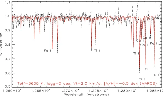
Figure 2.Example of a spectral window exploited to compare synthetic(solid line) and observed (dotted–dashed line) spectra. Key diagnostics for abundances are marked(Fe, Ca, and Ti).
wavelength regions, from 11700 to 13000Å. We determined a heliocentric velocity of RV=−105.2±2.0 km s−1(based on 34 spectral lines), which agrees quite well with the cluster average value given by Harris’s catalog (1996, 2010 update36) of −107.5±0.9 km s−1 and by Simmerer et al. (2013) of −104.03±5.03 km s−1. Note that the velocity amplitude of the Miras minimally affects thisfinding, since their typical variation is ∼10 km s−1 (Wood1979). Since our spectral coverage does not grant the inclusion of a sufficient number of FeI and (most crucially) FeII lines, the atmospheric parameters were adopted from photometric properties. More specifically, effective temper-ature(Teff) was obtained using J−Kscolors and the calibration by Alonso et al. (1999), assuming the reddening value from Harris
(1996) of E(B − V )=0.45, which corresponds to E(J − Ks)= 0.23 based on the extinction law of Cardelli et al.(1989). In order
to estimate the pulsation phase, we used the ASAS-SN light curve (Shappee et al. 2014; Kochanek et al. 2017), which covers the
epoch of our spectroscopic observation well (330 phase points from 2016 March to 2017 July; period of the Mira P=202 days from Sloan et al. 2010). Although the angular resolution of the
ASAS-SN is low(15 arcsec) for our target in the GC, its light curve clearly indicates that the target was near a minimum and the V-band magnitude is estimated at 15.3±0.1mag. Unfortunately, we have no recent infrared photometry for the target, and thus we used a light curve obtained at 1.4 m Infrared Survey Facility about 10 years ago. Matsunaga (2006) obtained 49 photometric points
which show periodic variation from 2002 March to 2005 August with an amplitude of∼0.4mag in Ks. Assuming that the phase lag between V-band and K-band light curves is 0.0–0.2 (with V preceding; see, e.g., Smith et al.2006), the K-band phase for the
spectroscopic data is 0.3–0.1cycles before the minimum leading to J−Ks=1.3±0.05 mag and Ks=8.9±0.15 mag from the IRSF light curve. V−Ks is then 6.4±0.2mag, which corresponds to (V − Ks)0=5.1±0.4 mag, while (J − Ks)0= 1.05±0.05 mag, with the reddening corrected.
We obtained a Teff=3600 K using the J−Ks colors and 3500 K using the V−Kscolors and the calibration by Bessell et al. (1998). We adopted the former one, since the NIR
photometry was collected simultaneously. The J−Ks is also less prone to reddening uncertainties when compared with V−Ks color, since E J( -K) E V( -K) = 0.19 mag (Cardelli et al. 1989). An error of 100 K is thus a plausible
uncertainty. We also applied the temperature scale based on the reddening-free method of line-depth ratios constructed by Taniguchi et al.(2018). Some lines of their 81 line pairs cannot
be measured in the crowded spectrum of V1 in NGC5927; however, we estimated Teff=3665±63 K. The current value is consistent with the estimate based on the color–temperature transformations, thus suggesting that they are minimally affected by a possible reddening variation and/or dust formation in warm Miras. Note that this temperature estimate was slightly extrapolated, since the temperatures of the calibrating stars used by Taniguchi et al. (2018) range from
3780 to 5400 K.
From the photometric Teff, assuming a mass of M=0.6Me, a true distance modulus of μ=14.44 mag (Harris1996), and
the bolometric correction for K magnitudes by Buzzoni et al. (2010), we estimated the surface gravity of log g=0.0±0.2,
where the error comprises contributions from all of the different sources of uncertainty (i.e., temperature, luminosity). A
microturbulence of ξ=2.0 km s−1 was set, following pre-scriptions from the literature for this kind of cool, giant star (e.g., Origlia et al.2013); note also that Nowotny et al. (2010)
and Lebzelter et al.(2014) imposed a value of ξ=2.5 km s−1
for Miras, in agreement, within the errors, with our value(see Table1).
3.2. Abundance Analysis
The determination of elemental abundances was carried out via spectral synthesis calculations using the driver synth in
MOOG by C.Sneden (1973, 2017 version) and the MARCS grid of spherical model atmospheres (Gustafsson et al.2008),
with α enhancements. The above mentioned atmospheric parameters were adopted, along with a global metallicity in the model atmosphere of [M/H]=−0.537 (see Harris’s catalog). The following crucial step includes the building of the line list. We carefully selected only atomic lines that are proven to be relatively isolated, unblended, and not affected by departures from local thermodynamical equilibrium(LTE). Our spectrum encompasses several KIlines, but we discarded this species since non-LTE corrections are not available for the lines under scrutiny (i.e., λ = 11772.838, 12432.27, and 12522.134Å). Moreover, we only kept lines that provide abundances for the Sun (Teff=5770 K, log g= 4.44, ξ=0.9 km s−1, [M/H]=0; D’Orazi et al. 2017) and
Arcturus (Teff=4286 K, log g=1.66, ξ=1.74 km s−1, [M/H]=−0.52; Ramírez & Allende Prieto 2011) in
com-pliance with literature values: all our measurements are in agreement within 0.1 dex with Asplund et al. (2009) and
Ramírez & Allende Prieto (2011), respectively. Our choice,
though limiting the number of lines and species that can be measured, allows us to infer reliable abundance measurements, with no major systematics affecting our values. Ourfinal line list includes NaI, FeI, SiI, CaI, and TiIlines and is given in Table2, where we report for each line the atomic parameters,
Table 1
Stellar Parameters(Teff, logg, andξ) and Abundances for Our Target Star
Mira V1 Cluster Average
α 15h28m15 2 L δ −50°38′09 0 L Ksa(mag) 8.9±0.15 L A Ksa(mag) ∼0.4 L Pb(days) 202 L Teff(K) 3600±100 L g log (cgs) 0.00±0.20 L ξ (km s−1) 2.0±0.5 L [Fe/H] −0.55±0.15 −0.47±0.06 [Na/Fe]c +0.35±0.20 +0.18±0.13 [Si/Fe] +0.14±0.15 +0.24±0.08 [Ca/Fe] +0.13±0.20 +0.15±0.04 [Ti/Fe] +0.17±0.13 +0.32±0.06
Notes.The corresponding uncertainties are given (see the text for details). The last column gives the cluster average abundances along with the standard deviation by Mura-Guzmán et al.(2018).
a
Mean Ks-band magnitude and amplitude(Matsunaga2006).
b
Sloan et al.(2010).
c
Element affected by p-capture reactions.
36
http://physwww.mcmaster.ca/~harris/mwgc.dat
37
We adopt the standard notation for abundances, whereby[X/H]=A(X)− A(X)eand A( )X =log(NX NH)+12.
i.e., excitation potential and loggf. The latter comes from different literature sources, including values by Kurucz38and the most recent computations for TiI lines by Lawler et al. (2013). In order to perform the comparison between observed
and synthetic spectrum, we have selected six wavelength regions with each interval covering ∼200Å: this means synthetic calculations for more than 1000Å, by covering all the spectral lines of interest. An example of a spectral region that we have selected for our chemical analysis is shown in Figure 2, whereas a zoom on the Ti line at 12,671Å is displayed in Figure 3. Our target has a low effective temperature and to properly locate the continuum we included molecular line lists for CH, CN, CO, and OH from B.Plez (private communication). The determination of C, N, O abundances is a tricky task because of their inter-dependency and because they are changing during the star’s evolution. To add further complications, since our star is a GC member, all the three elements under discussion are involved in the hot hydrogen burning that is commonly accepted to happen in a fraction of the cluster of first-generation stars (the so-called multiple population scenario; see Gratton et al. 2012 for an extensive review). Moreover, the WINERED spectral coverage does not grant the inclusion of the CO bandhead and/or OH features located in the H and K bands, which are commonly used to derive abundances for carbon and oxygen. Conversely, our spectra are populated with a large number of CN features. Thus, it is not straightforward to get insights on the initial content for C, N, O and on the amount of depletion/ enhancement that has occurred as the star gets evolved. For current purposes, we computed a grid of different synthetic spectra assuming different CNO abundances and finding the
bestfit that minimizes the χ2. Note that this approach does not allow us to derive C, N, and O abundances, since different combinations can provide similarχ2values. We are taking into account these molecular features to improve the continuum determination.
Chemical abundances are affected by internal uncertainties due to two main sources of error:(1) uncertainties on the best-fit determination (that takes into account continuum displace-ment and line measuredisplace-ments) and (2) errors related to the adopted set of stellar parameters. For thefirst kind of error we adopted the standard deviation (rms) from the mean abun-dances as given from different spectral lines: typical values are in the range 0.07–0.10 dex. To estimate errors due to stellar parameters(Teff,log ,g ξ, and [M/H]) we have proceeded in the standard way, that is changing each parameter one by one and evaluating the corresponding variation on the resulting abundances. Thus, temperature, gravity, microturbulence, and global metallicity were changed by ±100 K, ±0.2 dex, ±0.5 km s−1, and ±0.1 dex; we found errors on the [X/Fe] ratios of 0.10–0.12 dex. We then added in quadrature the four different error contributions and calculated the final error related to bestfit and stellar parameters as
; 1 T g best 2 2 log 2 2 M H 2 eff s= s +s +s +sx+s[ ] ( )
see the result given in Table 1. We note that, given the very good agreement for benchmark stars such as the Sun and Arcturus, major systematic uncertainties should not affect our abundance values at a level larger than∼0.1 dex.
3.3. Results and Concluding Remarks
Our results are given in Table 1, along with the corresp-onding total uncertainty (best-fit procedure and errors due to stellar parameters). The metallicity, [Fe/H]=−0.55±0.15, is in good agreement, within the observational uncertainties, with previous determinations from optical spectroscopy of GC giant members. Harris(1996) gives for NGC 5927 a value of
[Fe/H]=−0.49, whereas Pancino et al. (2017) found a
slightly larger metal content, [Fe/H]=−0.39±0.04. Very recently, Mura-Guzmán et al. (2018) have presented
high-resolution, FLAMES/UVES observations for a sample of seven red giants in this cluster, reporting a mean metallicity of
Table 2
Atomic Line List for NaI(Species=11.0), SiI(14.0), CaI(20.0), TiI(22.0), and FeI(26.0) Lines that We Used for the Abundance Analysis
Wavelength Species E.P. loggf [X/H]
(Å) (eV) 12,679.144 11.0 3.614 −0.04 −0.20 12,679.144 11.0 3.614 −1.34 L 12,679.224 11.0 3.614 −2.65 L 11,984.198 14.0 4.926 +0.19 −0.55 11,991.568 14.0 4.916 −0.16 −0.35 12,816.046 20.0 3.907 −0.63 −0.40 12,823.868 20.0 3.907 −0.85 −0.45 11,780.542 22.0 1.442 −2.17 −0.55 11,797.186 22.0 1.429 −2.28 −0.15 11,892.768 22.0 4.175 −2.17 −0.15 11,949.547 22.0 1.442 −1.57 −0.55 12,569.571 22.0 2.173 −2.05 −0.45 12,671.092 22.0 1.429 −2.52 −0.55 12,738.370 22.0 4.803 −2.35 −0.25 12,738.477 22.0 4.728 −1.25 L 12,811.480 22.0 2.159 −1.39 −0.55 12,821.672 22.0 1.459 −1.19 −0.40 12,831.442 22.0 1.429 −1.49 −0.55 12,840.607 22.0 4.660 −2.85 −0.25 12,847.033 22.0 1.442 −1.55 −0.35 11,882.846 26.0 2.196 −2.17 −0.51 12,190.100 26.0 3.632 −2.73 −0.60 12,648.943 26.0 6.395 −2.69 −0.54
Note.The [X/H] ratios are given in the last column.
Figure 3.Zoom on the TiIline at 12671Å. Different spectral syntheses (solid lines) are for [Ti/Fe]=0.00±0.2, compared with the observed spectrum (dotted–dashed line).
38
[Fe/H]=−0.47±0.02 (error of the mean, with rms=0.06 dex). Concerning the other chemical species, the cluster is included in the Gaia ESO survey, but Pancino et al. (2017) have published abundances only for Mg and Al (see
their Table2).
On the other hand, Mura-Guzmán et al.(2018) have derived
abundances for iron-peak,α, and heavy elements (e.g., Ba and Eu). In the last column of Table 1 we show their values of [X/Fe] ratios for the species in common with the present study. The two sets of elemental abundances agree quite well. Titanium and silicon abundances are slightly higher in Mura-Guzmán et al. (2018), but are still compatible within the
uncertainties, whereas there is an excellent agreement between the two Ca measurements. The current findings suggest a modest α-enhancement, less than ∼0.2 dex. Red giant branch stars in the Bulge display a steady decrease in α-enhancement as a function of the iron content (Gonzalez et al. 2011)
approaching solar abundances ([α/Fe]∼0) in the metal-rich regime([Fe/H] 0). The trend for GCs—targets that are old (t 10 Gyr) and almost coeval—for iron abundances higher than−0.7 dex is not well established, due to their paucity and the limited number that has been spectroscopically investigated (Zoccali & Valenti 2016). However, the current estimate
suggests that NGC5927 is located in the lower envelope of the α-enhancements typical of GCs (Pritzl et al. 2005; Mura-Guzmán et al. 2018).
As for Na, we obtained [Na/Fe]=0.35±0.20, to be compared with 0.18±0.13 of the cluster average. The sodium content deserves a specific discussion. There is a debate in the literature as to whether second-generation (i.e., Na-rich) asymp-totic giant branch stars do exist (see, e.g., Campbell et al.2013; Lapenna et al. 2015; MacLean et al. 2016; Wang et al.
2016). The Na abundances reported by Mura-Guzmán et al.
(2018) are corrected for departures from LTE following
prescriptions given in the INSPECT database39 that are not available for our NaI line at 12,679Å. Thus, this could in principle explain part of the discrepancy with our value; however, there is another critical point that has to be considered. Na is one of the species involved in proton-capture reaction processes that occur in GCs. All the GCs with a sufficient number of stars analyzed display internal variation in Na (e.g., Gratton et al. 2012). In particular, while the first-generation stars have
Na in agreement withfield stars (at the corresponding metallicity), the second-generation GC stars exhibit a significant Na enhancement. At the current stage, we cannot confirm (or disprove) that Mira V1 in NGC 5927 belongs to the second-generation cluster because we lack a control sample of red giants acquired with the same instrument.
The abundance analysis of Mira stars has been affected by a number of long-standing problems: incompleteness of atomic and molecular line list (Uttenthaler et al. 2015),
inhomoge-neous atmospheres and complex circumstellar envelops (Hron et al. 2015), together with nonlinear phenomena in the cool
molecular region located between the photosphere and the expanding molecular shell. These issues and the impact of both hydrostatic and dynamical models have been addressed in detail by Lebzelter et al.(2015). These difficulties are at least
partly reduced because we are dealing with a Mira that is on average warmer than typical Miras. The interesting finding in the current approach is the similarity between optical and NIR
abundance scale in spite of the difference in the adopted spectroscopic diagnostics. However, a more quantitative analysis of the impact of 1D versus 3D and static versus dynamical atmosphere models(Chiavassa et al.2018) would be
highly desirable in view of the unprecedented opportunity to observe Mira stars in Local Volume galaxies with the next generation of ELTs(Bono et al.2017).
We thank the staff of La Silla Observatory, European Southern Observatory, in Chile for their support during our observations. The development and operation of WINERED have been supported by MEXT Programs for the Strategic Research Foundation at Private Universities (Nos. S0801061 and S1411028) and Grants-in-Aid, KAKENHI, from Japan Society for the Promotion of Science (JSPS; Nos. 16684001, 20340042, 2184005, and 2628028). We thank the anonymous referee for positive and pertinent suggestions on the early draft of this Letter. This work was supported by Sonderforschungs-bereich SFB 881 The Milky Way System(subproject A3, A5) of the German Research Foundation(DFG).
ORCID iDs V. D’Orazi https://orcid.org/0000-0002-2662-3762 G. Bono https://orcid.org/0000-0002-4896-8841 V. F. Braga https://orcid.org/0000-0001-7511-2830 M. Monelli https://orcid.org/0000-0001-5292-6380 M. Bergemann https://orcid.org/0000-0002-9908-5571
M. Dall’Ora https://orcid.org/0000-0001-8209-0449
M. Fabrizio https://orcid.org/0000-0001-5829-111X G. Fiorentino https://orcid.org/0000-0003-0376-6928 Y. Ikeda https://orcid.org/0000-0003-2380-8582 M. Jian https://orcid.org/0000-0002-5649-7461 M. Marengo https://orcid.org/0000-0001-9910-9230 J. Neeley https://orcid.org/0000-0002-8894-836X J. L. Prieto https://orcid.org/0000-0003-0943-0026 C. Sneden https://orcid.org/0000-0002-3456-5929 T. Tsujimoto https://orcid.org/0000-0002-9397-3658 E. Valenti https://orcid.org/0000-0002-6092-7145 References
Alonso, A., Arribas, S., & Martínez-Roger, C. 1999,A&AS,140, 261
Asplund, M., Grevesse, N., Sauval, A. J., & Scott, P. 2009,ARA&A,47, 481
Bessell, M. S., Castelli, F., & Plez, B. 1998, A&A,333, 231
Bono, G., Braga, V. F., Ferraro, I., et al. 2017, in IAU Symp. 316, Formation, Evolution, and Survival of Massive Star Clusters, ed. C. Charbonnel & A. Nota(Cambridge: Cambridge Univ. Press),36
Buzzoni, A., Patelli, L., Bellazzini, M., Pecci, F. F., & Oliva, E. 2010,
MNRAS,403, 1592
Campbell, S. W., D’Orazi, V., Yong, D., et al. 2013,Natur,498, 198
Cardelli, J. A., Clayton, G. C., & Mathis, J. S. 1989,ApJ,345, 245
Carretta, E., Bragaglia, A., Gratton, R., D’Orazi, V., & Lucatello, S. 2009,
A&A,508, 695
Chiavassa, A., Casagrande, L., Collet, R., et al. 2018, A&A, in press (arXiv:1801.01895)
Clement, C. M., Muzzin, A., Dufton, Q., et al. 2001,AJ,122, 2587
Da Silva, R., Lemasle, B., Bono, G., et al. 2016,A&A,586, A125
D’Orazi, V., Desidera, S., Gratton, R. G., et al. 2017,A&A,598, 19
Fiorentino, G., Bono, G., Monelli, M., et al. 2015,ApJL,798, L12
Frogel, J. A., & Whitelock, P. A. 1998,AJ,116, 754
Gonzalez, O. A., Rejkuba, M., Zoccali, M., et al. 2011,A&A,530, A54
Gratton, R. G., Carretta, E., & Bragaglia, A. 2012,A&ARv,20, 50
Gullikson, K., Dodson-Robinson, S., & Kraus, A. 2014,AJ,148, 53
Gustafsson, B., Edvardsson, B., Eriksson, K., et al. 2008,A&A,486, 951
Harris, W. E. 1996,AJ,112, 1487
Hron, J., Uttenthaler, S., Aringer, B., et al. 2015,A&A,584, A27
Ikeda, Y., Kobayashi, N., Kondo, S., et al. 2016,Proc. SPIE,9908, 99085Z
39
Kochanek, C. S., Shappee, B. J., Stanek, K. Z., et al. 2017,PASP,129, 104502
Kunder, A., Stetson, P. B., Cassisi, S., et al. 2013,AJ,146, 119
Lapenna, E., Mucciarelli, A., Ferraro, F. R., et al. 2015,ApJ,813, 97
Lawler, J. E., Guzman, A., Wood, M. P., Sneden, C., & Cowan, J. J. 2013,
ApJS,205, 11
Lebzelter, T., Nowotny, W., Hinkle, K. H., et al. 2015, in ASP Conf. Ser. 497, Why Galaxies Care about AGB Stars III: A Closer Look in Space and Time, ed. F. Kerschbaum, R. F. Wing, & J. Hron(San Francisco, CA: ASP),283
Lebzelter, T., Nowotny, W., Hinkle, K. H., Höfner, S., & Aringer, B. 2014,
A&A,567, A143
MacLean, B. T., Campbell, S. W., De Silva, G. M., et al. 2016,MNRAS,460, L69
Martínez-Vázquez, C. E., Stetson, P. B., Monelli, M., et al. 2016,MNRAS,
462, 4349
Matsunaga, N. 2006, PhD thesis, The University of Tokyo
Matsunaga, N., Feast, M. W., & Menzies, J. W. 2009,MNRAS,397, 933
Mura-Guzmán, A., Villanova, S., Muñoz, C., & Tang, B. 2018, MNRAS,
474, 4541
Nowotny, W., Höfner, S., & Aringer, B. 2010,A&A,514, A35
Origlia, L., Oliva, E., Maiolino, R., et al. 2013,A&A,560, A46
Otsubo, S., Ikeda, Y., Kobayashi, N., et al. 2016,Proc. SPIE,9908, 990879
Pancino, E., Rejkuba, M., Zoccali, M., & Carrera, R. 2010,A&A,524, A44
Pancino, E., Romano, D., Tang, B., et al. 2017,A&A,601, A112
Pritzl, B. J., Venn, K. A., & Irwin, M. 2005,AJ,130, 2140
Ramírez, I., & Allende Prieto, C. 2011,ApJ,743, 135
Sameshima, H. 2018, PASP, submitted
Shappee, B. J., Prieto, J. L., Grupe, D., et al. 2014,ApJ,788, 48
Simmerer, J., Feltzing, S., & Primas, F. 2013,A&A,556, A58
Sloan, G. C., Matsunaga, N., Matsuura, M., et al. 2010,ApJ,719, 1274
Smith, B. J., Price, S. D., & Moffett, A. J. 2006,AJ,131, 612
Sneden, C. A. 1973, PhD thesis, The Univ. Texas
Taniguchi, D., Matsunaga, N., Kobayashi, N., et al. 2018, MNRAS, 473, 4993
Uttenthaler, S., Blommaert, J. A. D. L., Wood, P. R., et al. 2015,MNRAS,
451, 1750
Wang, Y., Primas, F., Charbonnel, C., et al. 2016,A&A,592, A66
Wood, P. R. 1979,ApJ,227, 220
![Figure 3. Zoom on the Ti I line at 12671Å. Different spectral syntheses (solid lines ) are for [Ti/Fe]=0.00±0.2, compared with the observed spectrum (dotted–dashed line).](https://thumb-eu.123doks.com/thumbv2/123dokorg/8052742.123297/5.918.65.444.126.519/figure-different-spectral-syntheses-compared-observed-spectrum-dashed.webp)
