A Multi-instrument Analysis of a C4.1 Flare Occurring in a δ Sunspot

(1)

819

(2)

A MULTI-INSTRUMENT ANALYSIS OF A C4.1 FLARE OCCURRING IN A

δ SUNSPOT

S. L. Guglielmino1, F. Zuccarello1, P. Romano2, A. Cristaldi3,4, I. Ermolli4, S. Criscuoli5, M. Falco1, and F. P. Zuccarello6

1

Dipartimento di Fisica e Astronomia—Sezione Astroﬁsica, Università di Catania, via S. Soﬁa 78, I-95123 Catania, Italy 2

INAF—Osservatorio Astroﬁsico di Catania, via S. Soﬁa 78, I-95123 Catania, Italy

3_{Dipartimento di Fisica, Università di Roma Tor Vergata, via della Ricerca Scientiﬁca 1, I-00133 Rome, Italy} 4

INAF—Osservatorio Astronomico di Roma, via Frascati 33, I-00040 Monte Porzio Catone, Italy 5_{NSO—National Solar Observatory, 3665 Discovery Drive, Boulder, CO 80303, USA} 6

LESIA, Observatoire de Paris, PSL Research University, CNRS, Sorbonne Universités, UPMC Univ.Paris 06, Univ.Paris Diderot, Sorbonne Paris Cité, 5 place Jules Janssen, F-92195 Meudon, France

Received 2015 September 15; accepted 2015 December 22; published 2016 March 9

ABSTRACT

We present an analysis of multi-instrument space- and ground-based observations relevant to a C4.1 solarflare that occurred in the active region(AR) NOAA 11267 on 2011 August 6. Solar Dynamics Observatoryobservations indicate that at the flare’s beginning, it was localized in the preceding sunspot of the AR, which exhibits a δ configuration. Along the polarity inversion line between its opposite polarities we find a large shear angle of about 80°. The helicity accumulation shows that the AR does not obey the general hemispheric helicity rule. At the flare peak, unique observations taken with the X-Ray Telescope aboard Hinode reveal that the bulk of the X-ray emission takes place in theδ-spot region, where the plasma heats up to 1.9 10_» _· 7_{K. During the gradual phase, we}

observe the development of a Y-shaped structure in the corona and in the high chromosphere. An extruding structure forms, being directed from the emitting region above the δ spot toward the following sunspot. This structure cools down in a few tens of minutes while moving eastward along a direction opposite to theflare ribbon expansion. Finally, remote brightenings are found at the easternmost footpoint of this structure, appearing as a third flare ribbon in the chromosphere. After some minutes, RHESSI measurements show that the X-ray emission is localized in the region close to the crossing point of the coronal Y-shaped structure. Simultaneously, high-resolution(0 15) observations performed at the Swedish 1 m Solar Telescope indicate a decreasing trend of the CaIIH intensity in theflare ribbons with some transient enhancements. All these findings suggest that this event is

a manifestation of magnetic reconnection, likely induced by an asymmetric magnetic conﬁguration in a highly sheared region.

Key words: Sun: activity– Sun: chromosphere – Sun: ﬂares – Sun: photosphere – sunspots – techniques: high angular resolution

Supporting material: animation

1. INTRODUCTION

Complex active regions(ARs) are the preferred location for activity phenomena of energy release occurring in the Sun. In particular, δ spots that are characterized by the presence of umbrae with opposite polarity inside the same penumbra host the majority of M- and X-class solarﬂares (e.g., Tanaka1991; Sammis et al.2000; Benz2008; McIntosh & Leamon2014).

A wide literature concerns the mechanisms that lead to the occurrence of flares in δ spots. A key point seems to be magnetic complexity, invoking magnetic reconnection between colliding flux tubes as a possible triggering process (e.g., Sturrock et al. 1984). Indeed, the non-potential magnetic field topology is thought to be responsible for the sudden release of the free magnetic energy taking place around the sheared polarity inversion line (PIL; Hagyard et al. 1984; Patty & Hagyard 1986; Machado et al. 1988; Mandrini et al. 1993; Schmieder et al. 1994; Liu & Zhang 2001; Leka & Barnes 2003; Tian et al.2005), through the interaction of the opposite-orientedflux systems or due to the compact electrical currents generated in the presence of high-gradient magnetic fields (Schrijver2007). The evolution of the magnetic shear in complex emergingflux regions is studied in several numerical simulations(e.g., Linton et al.1998,1999; Fan & Gibson2004; Zaqarashvili et al. 2010; Fang et al. 2012a, 2012b; Toriumi

et al. 2014). In particular, the recent model of Fang & Fan (2015) has been able to reproduce strong transverse ﬁelds with highly sheared magnetic and velocity ﬁelds at the δ-spot PIL with strong currents that are built up in this site.

In the standard CSHKP flare model (Carmichael 1964; Sturrock1966; Hirayama1974; Kopp & Pneuman 1976), the flare ribbons are the consequence of accelerated particles flowing down along reconnected magnetic field lines, generat-ing ribbon-shaped brightengenerat-ings in the denser lower layers of the solar atmosphere (e.g., Priest & Forbes 2002). They separate with time as they are the result of sequentially reconnected loop arcades that are located at higher and higher atmospheric layers. Such expansion, perpendicular to the PIL, is supported by observational evidence (e.g., Fletcher & Hudson2001; Moore et al. 2001; Fletcher et al. 2004).

However, the dynamics of the reconnectingfield lines during flares in ARs with intricate magnetic configurations, such as δ spots, also seem to be complicated by the effect of the slipping reconnection phenomenon(Aulanier et al.2006), which stands in the way of the traditional “cut-and-paste” reconnection occurring with an instantaneous change of connectivity.

Therefore, the characterization of the evolution of ﬂares occurring inδ spots and other complex magnetic conﬁgurations is very useful to clarify the dynamics of these solar events, providing through observations new insights useful to

(3)

phenomena and new constraints for ﬂare models (Fletcher et al.2011).

In this paper, we report the results concerning the analysis of a C4.1 classﬂare that occurred in AR NOAA 11267 (hereafter AR 267) whose main preceding sunspot showed a δ conﬁguration. The evolution of the AR 267 has already been described by Cristaldi et al. (2014) who analyzed a data set with very high spatial resolution (0 15) acquired at the Swedish 1-m Solar Telescope(SST) on 2011 August 6. They studied in detail the morphological, magnetic, and dynamic properties of the region between the opposite polarities of theδ spot in the photosphere, using the observations in the FeI557.6

and 630.15 nm lines. They found evidence of persistent upﬂows and downﬂows of about 3 km s-1_{in proximity of the}

δ-spot PIL. These motions, lasting about 15 hr, were interpreted as being due to Evershed flows occurring in the wrapped penumbralfilaments located in the region between the opposite polarities of theδ spot. However, Cristaldi et al. (2014) did not study the C4.1flare occurring in AR 267, which peaked some minutes before the beginning of the high-resolution observations.

Here, we investigate this ﬂare to determine the physical mechanisms underlying the event, e.g., the conditions under which magnetic reconnection sets in and how this evolves as theﬂare proceeds, and the response of the different atmospheric levels. We aim to provide new observational evidence as well, extending the number of events whose properties are studied in detail.

To this purpose we use a multi-wavelength approach. We analyze the same data set acquired at the SST in the photosphere used by Cristaldi et al. (2014) and we add new information by analyzing the FeI630.15 nm line as well as the

simultaneous CaII H chromospheric observations of the

evolution of the flare during the gradual phase. We also benefit from simultaneous observations in the ultraviolet and magnetic information provided by the the Solar Dynamics Observatory(SDO) satellite, which covers the entire flare evolution. Moreover, we analyze unique high-resolution data, not saturated at theflare peak, acquired by the X-Ray Telescope (XRT) on board the Hinode satellite, and we benefit from hard X-ray(HXR) measurements carried out by the RHESSI satellite that cover the gradual phase of theflare. The paper is organized as follows: in Section2 we describe the observations and in Section3we report the results of the data analysis coming from the different instruments. In Section4we discuss ourfindings in the framework of previous flare observations and models, bringing the pieces of information into a unified description of the C4.1flare, drawing our conclusions in Section5.

AR 267 appeared on the solar disk on 2011 August 4. It was classified as a bgd group and hosted five C-class flares during its lifetime, which was slightly shorter than a week. The strongest flare, classified as a C4.1 class flare by the flux emission measured by the GOES-15satellite, began at 08:37 UT and peaked at around 08:47 UT on 2011 August 6. We describe the data sets used to characterize this event in the following paragraphs. In Table 1 we summarize the data sources available for the analysis.

2.1. High-resolution Ground-based Observations The SST (Scharmer et al. 2003) acquired high-resolution data on 2011 August 6 from 09:00:05 UT until 09:37:37 UT, during the gradual phase of the C4.1ﬂare, when the AR was at solar coordinates (−350″, −360″), with heliocentric cosine anglem = 0.84.

The CRisp Imaging SpectroPolarimeter (CRISP, Scharmer et al.2008) carried out spectroscopic measurements along the proﬁle of the FeI line at 557.6 nm and full Stokes proﬁle

measurements of the FeI pair at 630.2 nm. Filtergrams in the

core of the CaIIH line at 396.88 nm, with a passband of 110

pm, and in the adjacent wide band were acquired simulta-neously with the FeI data by the cameras along the blue

channel of the SST. The pixel size of the FeIdata was 0 059

pixel−1 at 557.6 nm, while that of CaII H ﬁltergrams was

0 034 pixel−1. The temporal cadence of each complete scan of the FeI lines was ∼28 s. As concerns the blue beam (CaII H

line core and wide band), the temporal cadence was 8.9 s. The ﬁeld of view (FOV) of these SST data sets is 57. 5 ´57. 3 .

For further details on the SST data sets, we defer the reader to Cristaldi et al.(2014), who provide more information about the spectral coverage of the SST/CRISP measurements and the data reduction procedure via the CRISPRED pipeline (de la Cruz Rodríguez et al.2015). Here, we only remind the reader that the application of the multi-object multi-frame blind deconvolution(MOMFBD, van Noort et al.2005) technique to these SST data sets ensured that near diffraction-limited spatial resolution was achieved(0 15 at 557.6 nm).

2.2. Space-based Observations

Full-disk continuum and longitudinal (line-of-sight, LOS) magnetograms taken by the Helioseismic and Magnetic Imager (HMI, Scherrer et al. 2012) on board the SDO (Pesnell et al.2012) in the FeIline at 617.3 nm with a resolution of 1″

were used to complement the high-resolution data set of the SST. The SDO/HMI data used in this analysis cover three days

(4)

of observations, starting from 2011 August 5 at 00:10:25 UT until August 7 at 23:58:25 UT, with a cadence of 12 minutes (ﬁltergrams constructed from the HMI vector magnetic ﬁeld series). All the SDO/HMI images were aligned, taking into account the solar differential rotation, by using the IDL SolarSoft package.

In order to analyze in more detail the magnetic configuration of the AR during theflare, we also benefited from SDO/HMI Space-weather Active Region Patches(SHARPs) data (Hoek-sema et al. 2014). These SHARP data provide maps of the photospheric vector magnetic field of the AR and its uncertainty, computed using the Very Fast Inversion of the Stokes Vector code (VFISV; Borrero et al. 2011). The continuum intensity, Doppler velocity, and LOS magnetic field are also provided. See Bobra et al. (2014) for a comprehensive explanation of the SHARP pipeline. We corrected the SHARP data for the rotation angle of 180° of SDO/HMI data, and the vector magnetic field components were transformed into the local solar frame according to Gary & Hagyard (1990) using the proper SDO/HMI procedure (Sun 2013). Finally, we selected a subFOV of these data of about 129 ´91 encompassing the AR 267.

Data taken by the Atmospheric Imaging Assembly (AIA, Lemen et al.2012) aboard the SDO mission were used to study in detail the evolution of the ﬂare in the coronal and upper chromospheric layers. We extracted a series of cutout images with a FOV that covers 129 ´91, the same used for the SHARP data. These SDO/AIA cutouts comprise the time interval between 08:00 UT and 10:00 UT on August 6, with the highest available cadence(12 s for the EUV passbands, 24 s for the UV 1600Å images).

The XRT (Golub et al. 2007) aboard the Hinode satellite (Kosugi et al. 2007) was observing nearly the full solar disk, including AR 267, through the Ti/poly filter. The Hinode/ XRT had been operating in patrol mode since 08:17 UT. During the flare peak at 08:47 UT, it activated the target-of-opportunity mode and acquired a short series of filtergrams at higher resolution in four filters with a cadence of 22.2 s. The Hinode/XRT acquired 4 filtergrams through each of the Ti/poly and Al/mesh filters, with a pixel scale of 2 06, and 4filtergrams through each of the Al/thick and Be/thick filters, with a pixel scale of 1 03. For the latter filters, the exposure times are reported in the Table2.

The RHESSI (Lin et al. 2002) satellite was in night until 08:59 UT and after this time performed some measurements in the nine different energy channels. One event in theﬂare list of RHESSI, which has been attributed to AR 267, has two peak emissions occurring at 09:00:06 UT and at 09:11:38 UT. Both of these peaks fall within the SST observing time. In particular, theﬁrst peak at 09:00:06 UT, mostly visible in the low energy channels, i.e., at 3–6 and 6–12 keV, was by far more intense than the second one.

2.3. Alignment between Different Data Sets

SDO/AIA and SDO/HMI data were aligned with each other by using the IDL SolarSoft mapping routines to take into account the different pixel sizes. SST CaIIH and SST/CRISP

images were aligned by considering theﬁrst ﬁltergram in the adjacent wide band of the CaII H and the continuum image

deduced from the ﬁrst sequence taken by SST/CRISP in the FeI557.6 nm line acquired at 09:00:05 UT, which was already

aligned with the SST/CRISP data in the FeI630.2 nm pair by

means of the MOMFBD algorithm.

To co-align SST/CRISP and SDO observations, we used the ﬁrst spectral image in the sequence of SST/CRISP data taken in the continuum of the FeI557.6 nm line and the SDO/HMI

reference image in the continuum closest in time. The displacement between the two images was obtained with cross-correlation techniques. The alignment obtained was conﬁrmed by the correspondence between the ﬂare ribbons seen in the SST CaII H image taken at 09:00:05 UT and the

nearly simultaneous SDO/AIA image acquired at 1600 Å. We estimate that the precision of the alignment obtained by using this procedure is of the order of the pixel scale of SDO images, i.e., 0 5.

The Hinode/XRT filtergrams were aligned to the SDO/AIA images by using the first non-saturated filtergrams obtained through the Al/thick filter and the simultaneous SDO/AIA image acquired at 94Å at the flare peak. The displacement between these two images was obtained with cross-correlation techniques. The precision of such an alignment can be estimated as of the order of the resolution of these Hinode/ XRT measurements, about 2″. Finally, for RHESSI measure-ments, we used the pointing information provided by the instrument.

3. RESULTS

In thefirst place, we have looked at the evolution of some global properties of the AR 267 during its passage across the solar disk, which vary on timescales much larger than the C4.1 flare development. These help us to characterize the magnetic environment and its relation to theflare occurrence.

The observing context of our analyses is shown in Figure1. In thisfigure, we display an SDO/HMI continuum map of the photospheric configuration of AR 267 on 2011 August 6 at 08:58:25 UT, roughly at the time of the beginning of the SST observations. It is clearly visible that the preceding sunspot of AR 267 has aδ configuration, as shown by the contours of the simultaneous SDO/HMI longitudinal field map. The preceding spot exhibits a southern umbral core with negative polarity and a larger, northern core with positive polarity. In this SDO/HMI map we also indicate the subFOV covered by the SDO/HMI SHARP data and for SDO/AIA cutout data (dotted line), and the FOV of the SST observations(solid line).

In Figure2(top panel) we plot the X-ray emission flux in the 1–8 Å channel as measured by the GOES-15satellite from 00:10:25 UT on 2011 August 5 until 23:58:25 UT on August 7. Fiveflare events have been associated with activity phenomena in AR 267, whose time and magnitudes are also reported in Figure2(middle and bottom panels). The yellow vertical band drawn in all of the panels of Figure2 indicates the observing time of the SST high-resolution observations. The strongest flare in the AR 267, classified as C4.1, occurred a few minutes before the beginning of these ground-based observations.

Table 2

Acquisition and Exposure Times for the Series of Hinode/XRT Filtergrams Acquired at High Spatial Resolution During the Flare Peak

Time(UT) Al/thick Time(UT) Be/thick

08:47:35 1.024 08:47:40 2.049

08:47:56 0.725 08:48:00 2.899

08:48:19 1.025 08:48:23 5.797

(5)

Figure 2 (middle panel) shows the evolution of the total unsigned magneticflux in the whole AR 267 during the same time interval (black symbols). The magnetic flux has been deduced from SDO/HMI longitudinal magnetograms and computed using the full FOV of about 121 ´161 encom-passing AR 267, which is shown is Figure 1. We have also taken into account projection effects due to the variation of the heliocentric cosine angle μ. Moreover, the plot reports separately the flux in the subFOV encompassing only the δ spot(right half of the FOV shown in Figure1, at the right-hand side of the dashed vertical line). This allows us to distinguish the contribution of the positive (red symbols) and negative (blue symbols) flux in the δ-spot area due to flux emergence or disappearance. Note that during the first major flux decrease, when the SST was observing in the part of AR 267 encompassing theδ spot, the negative flux diminished whereas the positive flux was almost constant, around its maximum value at_~1.5_´1021_Mx.

In Figure 2 (bottom panel) we also plot the helicity accumulation trend for AR 267 during the same time interval, retrieved by the longitudinal ﬁeld measurements obtained by SDO/HMI in the full FOV shown in Figure1.

The magnetic helicity is a physical quantity that provides a measure of the complexity of the magnetic field configuration (see, e.g., Romano et al.2014). Although the direct computa-tion of magnetic helicity in an AR would require a complete knowledge of the entire magnetic field connectivity in the considered volume, a useful estimate of this quantity can also be derived from magnetic field measurements taken at the photospheric level. Indeed, we can obtain the magnetic helicity flux from the convection zone (dH/dt) by using the measure-ments of the vertical component of the magneticfield and the computation of the displacements of the photospheric magnetic structures as proposed by Pariat et al.(2005).

For the purposes of this investigation, we have computed the magnetic helicity accumulation in the AR 267 by estimating the magnetic helicity flux with the abovementioned method (Pariat et al.2005). To evaluate the horizontal displacements in the photosphere, we have followed the method described by Schuck(2008) by comparing the magnetic field between two magnetograms taken with a time interval of 12 minutes by means of the Differential Affine Velocity Estimator (Schuck 2005,2006), using an apodization window of 11 pixels (5 5) of full width at half maximum.

AR 267 shows a prevalent negative magnetic helicity accumulation during the observing time interval despite being located in the southern hemisphere. Hence, AR 267 does not obey the general cycle-invariant hemispheric helicity rule(Liu et al. 2014). At the time of the C4.1 ﬂare, the value of the helicity accumulation was_~-7.3_´1040Mx2_{. The monotonic}

Figure 1. SDO/HMI continuum intensity image showing the photospheric conﬁguration of AR 267 at 08:58:25 UT on 2011 August 6. Contours refer to

the simultaneous SDO/HMI longitudinal magnetogram—±500 G (yellow/

green contours) and ±1000 G (red/blue contours)—which highlights the presence of both positive and negative polarities in the preceding sunspot. The solid line square indicates the FOV of the SST acquisitions. The dotted line rectangle indicates the subFOV of SDO used for the analyses. The part of SDO FOV to the right of the dashed line was used to compute the magneticﬂux in the δ-spot area, as shown in Figure 2 (middle panel). In this and in the

following images, solar north is on the top, and west is at the right.

Figure 2. Top: GOES-15X-ray flux during the two days analyzed. Middle: total magneticflux (black symbols) and positive/negative magnetic flux (red/ blue symbols) in the region encompassing the δ spot of AR 267 during the two days considered. Bottom: helicity accumulation trend in AR 267 during the two days analyzed. In all of the panels, the yellow vertical band indicates the time interval covered by the SST high-resolution observations. The error bars in the plots of magneticflux and of helicity accumulation have been derived by propagating the SDO/HMI sensitivity of 10 G.

(6)

trend of the magnetic helicity accumulation in the corona until the occurrence of the last C1.6flare was supported by phases of magneticflux emergence (see Figure2, middle panel), but also could have involved peculiar horizontal velocity fields, in particular in theδ-spot region after the appearance of the bulk of the magnetic flux of AR 267.

3.1. Impulsive and Early Gradual Phase

To have diagnostic information about the ﬂare local magnetic environment and the properties of the energy release site, we have analyzed observations taken around the ﬂare peak.

A general survey of the magnetic configuration of the AR 267 in the photosphere during theflare is indeed useful to infer the vector magneticfield topology which could lead to the flare. Figure3(top panel) shows the SDO/HMI SHARP map of the longitudinal component of the vector magnetic field nearly at the time of theflare peak. The red (green) arrows indicate the direction of the transversal component in the positive (negative) polarity and their orientation follows the azimuth

direction. A strong magnetic shear is detected in the δ spot along the PIL separating the two umbrae of opposite polarities (thick orange line), as the magnetic ﬁeld is almost parallel to this PIL. The average value of the horizontal shear angle(see, e.g., Gosain & Venkatakrishnan2010) along the δ-spot PIL is about 80°. The shear angle was calculated considering a potential extrapolation according to Alissandrakis (1981). Diffuse, weak magnetic ﬁelds with opposite polarities are observed at the eastern and western edges of AR 267.

In order to obtain hints about the connectivity of the magneticfield lines of AR 267 in the upper atmospheric layers, we have computed a linear force-freefield extrapolation, again using the method of Alissandrakis (1981). We have chosen a value of the α parameter equal to 0 0025−1, which seems to reproduce in a better way the loops observed in the corona in the EUV(see Section3.2). Such a force-free field approxima-tion can be considered fairly representative of the overlying field, which does not appear to be strongly twisted (e.g., Régnier 2013). Although in the presence of magnetic field advection and cancellation at the photospheric level, in this manner we can have some information about the globalfield of AR 267. In Figure 3 (bottom panel) we display an image representing the result of this extrapolation. We find the presence of three different systems of magnetic field lines in AR 267: blue lines represent the field lines connecting the opposite polarities of theδ spot, red lines are those connecting the positive polarity of the δ spot with the following sunspot, and yellow lines are those connecting the positive polarity of theδ spot with the diffuse field of negative polarity to the south of the main negative polarity of AR 267.

The careful analysis of the GOES-15flux curves in the 1–8 Å channel, shown in Figure 4 (left panel, solid line), indicates that the C4.1 flare peaked at 08:47:37 UT, which is the time corresponding to the change in the sign of the derivative of the soft X-ray(SXR) flux. Moreover, we take the derivative of the SXR flux as proportional to the HXR flux, referring to the so-called “Neupert effect” (Neupert 1968). Looking for an increase in the HXRflux, we have estimated the beginning of the impulsive phase, which occurs at 08:37:51 UT. In addition, in Figure 4 (left panel) we display the GOES-15flux curves in the 0.5–4 Å channel (dotted line), which shows a similar temporal behavior.

Figure 4 (left panel, circles) also shows the light curve deduced from the Hinode/XRT measurements through the Ti/ poly filter: it has been obtained by taking the average of the X-ray intensity within the box indicated with a black line in the Hinode/XRT filtergrams displayed in Figure 4 (right panel). The quiet Sun regions indicated with gray boxes have been used to verify the genuineness of the X-ray signals that were not due to cosmic-ray contamination. The X-ray flux in these quiet Sun regions is negligible compared to the scale used for Figure4 (left panel).

When Hinode/XRT observed AR 267 at high resolution during theflare peak, there were filtergrams that did not go into saturation, although they were only those acquired through the Al/thick and Be/thick filters. This fact makes these Hinode/ XRT data unique, as very fewflares observed by the instrument have exposure times such that only the emission core is visible. All of the four images taken with the Hinode/XRT Be/thick filter were not saturated, while in the Al/thick filter only two images over the four filtergrams did not reach the saturation level, i.e., the ones with shorter exposure times(see Table2).

Figure 3. Top panel: SDO/HMI SHARP map of the Blongcomponent of the

vector magneticﬁeld of AR 267. The arrow length is proportional to the Btran

component of the vector magneticﬁeld, while their orientation indicates the azimuth direction. The arrow at the top-left corner of the map represents a Btran

component of 1000 G. The solid orange and light blue lines represent the PILs of the AR 267: the light blue one refers to the main PIL between the two main polarities of AR 267, and the orange one to the PIL between the opposite polarities of the δ spot. Bottom panel: force-free ﬁeld extrapolation (_{a = }0. 0025-1_{). See the text for the description of the color scheme referring} to the bundles ofﬁeld lines that describe the different connectivities present in AR 267.

(7)

Thus, in order to deduce the coronal temperature and the differential emission measure (DEM) we have summed over the two Al/thick images not saturated and the ratio has been calculated for the two Be/thick images closest in time. Indeed, we take advantage of the procedure proposed by Narukage et al.(2011) to estimate the temperature and DEM by means of theﬁlter ratio method using the SolarSoft routineXRT TEEM.PRO.

We adopt the calibration performed by Narukage et al.(2014) for those Hinode/XRT thick ﬁlters.

In Figure 5 (top panel) we display the X-ray intensity with the Al/thick filter at the flare peak. We can note that the bulk of the X-ray emission is located in the area corresponding to the δ-spot region ([−355″, −335″]×[−365″, −345″]). The plasma temperature is shown in Figure 5 (bottom panel): the average value in the flaring region is about 1.9 10· 7K, in agreement with predictions of flare models (see, e.g., Hirayama 1974). The mean value of the volume emission measure in the same region is 46.5 log cm-3_.

3.2. EUV Evolution

In this section of the analysis, we study the timing and spatial evolution of the structures as seen by SDO/AIA in the upper atmospheric layers to describe the development of the ﬂare. We have found an asymmetric evolution of the ribbons and the formation of a Y-shaped conﬁguration whose tail expands with time over the following sunspot of AR 267.

In Figure 6 we report a series of snapshots relevant to the C4.1 flare observed by SDO/AIA at different EUV wave-lengths around the flare peak at 08:47 UT and almost simultaneous to the SDO/HMI SHARP map shown in Figure3 (top panel). These images show the morphology of AR 267 at that time in various atmospheric layers. In the upper photo-sphere we are able to distinguish a pair of asymmetric ribbons (see the image at 1600 Å), while in the upper chromosphere we also detect some emission in between them (see the image at 304Å). In the corona the emission above the flaring region reaches the saturation level of the detectors for the majority of the EUV channels, i.e., at 171, 193, and 211Å. Only at 335 and 94Å can we note that the ribbons visible in the lower

atmospheric layers are overarched by coronal loops that connect them. At these wavelengths, the shape of AR 267 seems very similar to the one simultaneously observed in the X-rays by Hinode/XRT with lower spatial resolution (compare Figure6, at 335 and 94Å, with Figure5, top panel). Note that, as far as this study is concerned, the saturation present in almost all of the EUV channels does not complicate our analysis.

Interestingly, an extruding structure directed from theﬂaring region toward the eastern direction is seen at various

Figure 4. Left panel: X-ray light curve (gray circles) deduced from Hinode/XRT measurements through the Ti/poly ﬁlter in the region indicated with a black box in the image shown in the right panel, encompassing AR 267. Overplotted are the GOESﬂux curves in the 1–8 Å channel (solid line) and in the 0.5–4 Å channel (dotted line). Right panel: context image of Hinode/XRT observations in patrol mode. The black box encompasses AR 267; the gray boxes identify quiet Sun regions used as control regions.

Figure 5. Top panel: X-ray intensity map deduced from the Hinode/XRT. Bottom panel: plasma temperature at theﬂare peak deduced using the ﬁlter ratio method according to Narukage et al.(2014).

(8)

Figure 6. SDO/AIA intensity images at a time close to the C4.1 ﬂare peak. All the EUV maps are shown in reverse intensity scale. The dotted line box shown over the image at 304Å indicates the region used to compute the light curves plotted in Figure7. The colored segments that cross theﬂare ribbons are used to deduce the time slices discussed in Section3.2and shown in Figure8.

(9)

wavelengths: it is extremely evident in the image in the 131Å passband, which during ﬂares samples emission from mainly FeXXI lines(see, e.g., O’Dwyer et al.2010). The presence of

this feature gives rise to a Y-shaped structure in the corona above AR 267, which will become clearer in the subsequent minutes.

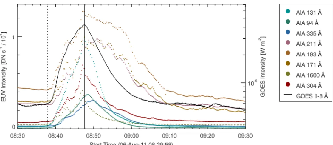
We have computed the light curves for all the SDO/AIA EUV channels and for the 1600Å ﬁltergrams, by averaging the SDO/AIA intensity within the box shown in Figure 6 in the image relevant to the 304Å channel (top-left panel). These light curves, which are displayed in Figure7, show that most of the EUV and UV intensities begin to increase at the time of the HXR emission, indicated with a dotted vertical line. The plot also points out the presence of some time delays between the intensity peaks in the different EUV channels between themselves and between the SXR emission measured by the GOESsatellite as the SDO/AIA intensities reach their maximum value at slightly different times.

In detail, the maximum intensity in the lower atmospheric layers, to which the 304 and 1600Å channels refer, is reached about 30 s before theflare peak in SXR, which is indicated with a solid vertical line in Figure 6. The maximum is almost simultaneous with the flare peak at 131 Å, the EUV filter relevant to the hottest plasma temperature. Moreover, at this wavelength the light curve is narrower than the others and exhibits a linear rise and decrease, the latter with a slope slightly steeper than the former. A similar linear trend is present in the light curve at 94Å, which, however, has a maximum about 60 s after theflare peak. The light curve at 335 Å has its maximum 120 s after the flare peak with a slow decrease. Finally, the 171, 193, and 211Å channels, which are strongly affected by saturation, exhibit a rapid rise phase, with a maximum almost simultaneous with theflare peak, and have a very long decrease phase. Table3 summarizes the time delays that are found between the intensity peaks in the light curves relevant to different EUV passbands, between them and the SXR emission.

To study the spatial evolution of the ﬂare ribbons in the δ-spot region, we have used intensity time slices. In the map shown in Figure 6 relevant to the 304Å channel (top-left panel), we have indicated three segments with different colors labeled with different letters (A, B, C), along which the intensity time slices have been derived. We show in Figure 8 the slices relevant to four SDO/AIA passbands that exhibit a

low degree of saturation: 335, 211, 1600, and 304Å. In these images, the bottom part of the slice refers to the southwestern point of the segments in Figure 6 and the top part to the northeastern point of the segments.

The activation of the emitting regions, which form the ribbons, occursfirst in segment A even if an emission kernel is present since the beginning of HXR emission in the northern ribbon along segment C. Then the emission in ribbons activates in segment B and eventually in segment C. The northern ribbon activates before the southern one. The ribbons’ activation also shows a delay between the atmospheric layers: it begins in the 1600Å channel, then it is seen at 304 Å, at 211 Å, and finally at 335Å. However, the southern ribbon along segment C activates simultaneously in all of the SDO/AIA channels, almost at the time of theflare peak at 08:47 UT.

Theflare ribbon motions are clearly recognized at 1600 and 304Å, along the segments B and C. We note both the effect of the drift of the northern ribbon outward of the δ-spot region, and the similar motion of the southern ribbon, when it appears, which results in the increasing flare ribbon separation. Note that the different slope in the drift of the ribbons indicates that the southern ribbon, when it appears, moves faster than the northern ribbon. The estimate of the speed, which has been derived from the 1600Å observations through a linear fit of the displacements of the intensity maxima in the ribbons, is of 1.05 and 1.75 km s-1 _{for the northern and southern ribbons,}

respectively.

Conversely, the emission in ribbons has already ended along segment A at 1600Å at the time of the ﬂare peak. After that time, in the upper chromosphere the bulk of emission ends along segment A, then in segment B, andﬁnally in segment C

Figure 7. SDO/AIA light curves for different channels, computed by averaging the intensity in the region indicated with a box in Figure6(top-left panel), relevant to

the 304Å passband. The dotted vertical line indicates the start of the ﬂare according to the HXR emission; the solid vertical line shows the ﬂare peak.

Table 3

Time Delays between Peaks in SDO/AIA Passbands and the SXR Peak

Passband Delay with SXR Peak

304Å −30 s 1600Å −30 s 171Å 0 s 193Å 0 s 211Å 0 s 335Å 120 s 94Å 60 s 131Å 0 s

(10)

(see the 304 Å passband). A similar progression is present in the upper atmospheric layers, as can be seen in the images relevant to the 211 and 335Å channels, but at these levels the emission decrease is slower than in the chromosphere.

These dynamics are highly suggestive of an asymmetric ribbon expansion. Besides separating each other, as usual, the ﬂare ribbons move toward the northeastern part of the δ-spot region along a direction that is perpendicular to that identiﬁed by the crossing segments A, B, and C shown in Figure6.

We have also derived the evolution of the extruding structure in all the UV/EUV channels using a slice along it as shown in

Figure9. This ﬁgure shows the map of AR 267 in the 131 Å passband at theﬂare peak. The red line indicates the slice that has been used for the subsequent analysis.

The behavior of the extruding structure in the various wavelengths is reported in Figure10. In thisfigure, the bottom part of each panel refers to the easternmost point along the slice, while the top part of the panels refer to the point of the slice closest to the δ spot. We can see that this structure first appears at 131Å, where it is observed for less than ten minutes since 08:44 UT, a few minutes before theflare peak (indicated in this panel with a black vertical line). Slightly after the flare peak, when the EUV intensity reaches its maximum at 131Å, the structure is also observed at 94Å: in this channel the emission is no longer detected after 09:00 UT. In both these channels, the emission kernel is at first observed near the δ spot. Then, the EUV intensity peak moves toward the following spot of AR 267, at wavelengths progressively referring to lower plasma temperature. The structure is observed at 335Å about five minutes after the flare peak, and the emission enhancement lasts for more than 30 minutes. We also note a very faint enhancement near theδ spot at 08:47 UT, at theflare peak, and in the 193 and 171 Å channels, which can be also found at 304 and at 1600Å. Much more evident is the sudden increase in brightness that is simultaneously detected at 211, 193, and 171Å at 08:57 UT, corresponding to the appearance of the extruding structure in these channels. This EUV emission increase is observed mostly near the following spot of the AR and it is dramatically strong at 171Å for a couple of minutes. After about one minute, an abrupt dimming at the chromospheric level is detected at 08:58 UT along the slice in the 304Å passband, which lasts for a few minutes. Other enhancements are observed at 09:06 UT and 09:10 UT at 193 and 171Å, which are located mostly near the following spot. Near theδ spot a new enhancement along the slice is seen at 09:10 UT in the 304Å passband with a short duration. The extruding structure is not found at 1600Å where, except for the brightening at the time of theflare peak, when we notice only slight enhancements toward theδ spot and the following spot of AR 267.

Figure 8. SDO/AIA intensity time slices. The color scheme refers to the colors of the segments indicated in Figure6at 304Å. The bottom (top) part of each panel refers to the southwestern (northeastern) point of the segments in Figure6. The dotted vertical line indicates the start of theﬂare and the solid vertical line represents theﬂare peak.

Figure 9. SDO/AIA map of AR 267 at 131 Å at a time close to the C4.1 ﬂare. The image is the same as in Figure6. The red line indicates the location of the intensity time slice along the extruding structure; the solid line box is the region where the EUV signal has been averaged to deduce the light curves shown in Figure11.

(11)

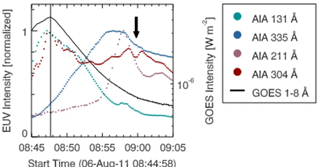
The evolution of the extruding structure has been further investigated by considering the average value of the EUV intensity in four passbands in a region encompassing the structure, framed by a solid box in Figure9. The resulting light curves are displayed in Figure11. The EUV intensity has been normalized to the maximum value of each passband in the time interval considered in the plots.

The intensity in the 131Å passband has a maximum at the time of the ﬂare peak, and only a slight increase during the decay phase, almost coincident with the maximum seen at

211Å, at 08:58 UT. A few minutes before, we ﬁnd the maximum in the 335Å channel, after a slow increase. The increase and the immediately subsequent dimming are clearly visible in the 304Å at 09:00 UT, as indicated by the arrow in Figure 11. Such a dimming is followed by a new, slight increase andﬁnally the intensity decreases.

In order to discuss the spatial evolution of the flare in different SDO/AIA passbands during the early gradual phase, we display in Figure12the isophotes of the EUV/UV emission at different times. Contours drawn in red color at 08:46 UT, at theflare peak, show strong, localized emission straggling over the δ-spot PIL (solid orange line). This emission reaches saturation levels in some EUV passbands. The flaring site is still localized, even if with a lesser extent over theδ-spot PIL at 08:53 UT(contours shown in green color). This is seen in the various channels, for instance at 211Å, but is more pronounced in the 304Å channel where the EUV emission is placed almost at the opposite sides of theδ-spot PIL. At the same time, we see the appearance of the extruding structure in the EUV channels referring to lower plasma temperature. It can be recognized as new emission regions appearing to the south of the main PIL of AR 267(solid light blue line in Figure12) almost parallel to it. This is particularly evident in the 211 and 335Å channels.

By the time SST observations began, the blue contours in Figure 12 referring to 09:00 UT indicate that the extruding structure was clearly formed and connected the initial flaring region, localized around the δ-spot PIL, to the following polarity of the AR 267. The structure appears to run parallel to the main PIL of the AR: this is distinctly seen at 211Å. At 335Å we find that the structure still occupies the same region that was occupied at 08:53 UT, while in the 1600Å passband we only see a small patch appearing in that region. In theδ-spot region, the EUV emission is now reduced in size, placed almost at the opposite sides of theδ-spot PIL also in the EUV channels referring to higher plasma temperature(335 and 211 Å). In the passband referring to the lower layers of the atmosphere, the EUV/UV emission is localized in small emission patches at the opposite sides of theδ-spot PIL (see the contours at 1600 and 304Å). Note that the apparent motion of the extruding structure eastward, i.e., of the EUV/UV enhancements, occurs along a direction that is nearly opposite to the direction of the flare ribbon expansion in the region of the δ-spot PIL.

3.3. Late Gradual Phase

In this section we benefit from high-resolution ground-based observations and RHESSI measurements, which cover only the late gradual phase of the C4.1 flare, since about 13 minutes from the beginning of theflare. We have studied the evolution

Figure 10. SDO/AIA intensity time slices along the extruding structure for different wavelengths. The slices refer to the region within the solid line box shown in the map reported in Figure9. The bottom of each panel corresponds to the easternmost part of the extruding structure, and the top of each panel correponds to the part closest to theδ spot. The dotted vertical lines indicate the start of theﬂare according to the HXR emission; the solid vertical lines are the ﬂare peak.

(12)

of the ribbons, theirﬁne structure magnetic environment, and the correlation of their spatial distribution with the presence of HXR sources.

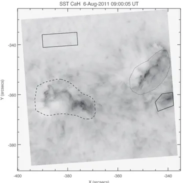
Figure13shows the chromospheric appearance of AR 267 in the core of the CaII H line at the beginning of the SST

observations (reverse intensity scale). It is possible to clearly distinguish three regions with enhanced emission, which correspond to the three apparent ribbons of theﬂare, encircled with lines.

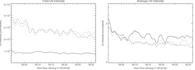
We have computed the light curves relevant to the three sites with enhanced emission observed in the chromosphere, high-lighted in Figure13. The plots shown in Figure14report the total UV intensity (left panel) and the average UV intensity (right panel), normalized for the background represented by the average value of the CaII H line core intensity within the

rectangular box overplotted in Figure13. For each of the three regions(see the line code in the caption), we have considered the total and the average value of the UV intensity only for those pixels with emission at least twice the value of the background intensity.

The two bigger regions, corresponding to the northern ribbon in theδ-spot region and to the ribbon in the following sunspot, respectively, exhibit a decreasing trend during the gradual phase for both the total intensity and the average intensity, as usually observed during the gradual phase. In contrast, we note that the small region corresponding to the southern ribbon in theδ spot shows an almost constant value in the total intensity, while the average intensity has some enhancements during the decrease. The strongest enhancement seems to be simultaneous with the second peak of X-ray emission observed by RHESSI at

Figure 12. SDO/HMI continuum ﬁltergram cospatial and simultaneous to the image shown in Figure3(top panel). The thick orange and light blue lines

represent the PILs of the AR 267, as in Figure3(top panel). The isocontours

refer to different observing times. Red: 08:46 UT, green: 08:53 UT, blue: 09:00 UT. The intensity value to which the contours refer is the same for each

SDO/AIA passband.

Figure 13. Map acquired in the CaIIH line core by the SST at 09:00:05 UT. Thefiltergram is shown in reverse intensity scale. The regions encircled with contours indicate the three regions with enhanced emission, which constitute the CaIIHflare ribbons. The line style of each region refers to Figure14. The rectangular box identifies the quiet Sun region considered as the background emission in these CaIIH observations.

(13)

09:11:38 UT. A similar spiky behavior, characterized by a timescale of a couple of minutes, can also be seen in the other two ribbons, concerning more clearly the total UV intensity. However, this can be in some measure due to variations in the seeing or to oscillations in the chromosphere (e.g., Jess et al. 2015) as it partially affects the background emission measured in the rectangular box of Figure 14.

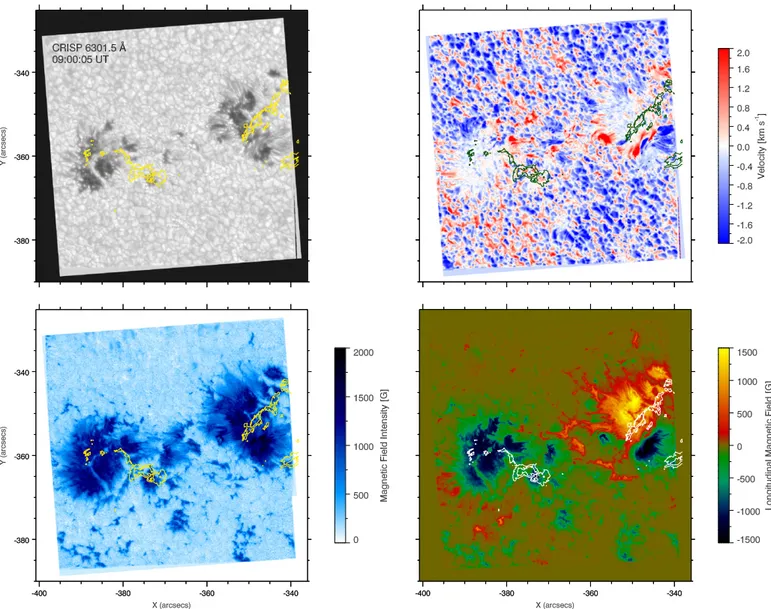
SST/CRISP observations provide new information concern-ing the photospheric conﬁguration of AR 267 during the gradual phase. In Figure15(top-left panel) the morphology of AR 267 at the beginning of SST/CRISP observations in the continuum of the FeI line at 603.15 nm is shown. We remind

the reader that the characteristics in the region around the δ-spot PIL in the photosphere have been extensively described by Cristaldi et al.(2014). Here, we note that the preceding and the following sunspots appear comparable in size and that light bridges are present in the umbral regions of both sunspots.

Figure15(top-right panel) displays the simultaneous map of Doppler velocity, which shows the plasma motions at a photospheric level in the AR 267. To derive the Doppler velocity, we have applied a Gaussianﬁt to the FeIline proﬁle

at 603.15 nm with the MPFIT routine (Markwardt 2009) in IDL. The local frame of rest was calibrated by imposing that plasma in the quiet Sun has, on average, the convective blueshift for the FeI 630.15 nm line (Dravins et al. 1981),

corrected for the position on the solar disk (m = 0.84) according to Balthasar (1988). We have used a value of_-235 m s-1_.

The map shows strong upflows and downflows in the region between the opposite polarities of the δ spot, as observed by Cristaldi et al. (2014) in other iron lines. At the easternmost extremity of the northern ribbon in theδ-spot region, we find an upflow of about 1.5 km s-1_.

Figure 15also shows the simultaneous maps of the magnetic field intensity (bottom-left panel) and of the longitudinal component of the magnetic field (bottom-right panel) of the entire SST FOV. These magneticfield maps have been deduced by applying the VFISV code, which performs a Milne– Eddington inversion of the data (Borrero et al. 2011), to the full SST/CRISP spectropolarimetric profiles along the FeI

630.15 nm line. The longitudinal component refers to the observer frame, and although it does not take into account the effects of projection, it is sufﬁcient for the scopes of our analysis.

Thefine structure of the tangled magnetic field in the δ-spot region is clearly revealed in the longitudinal field map. The magnetic field strength is of the same order of magnitude in the preceding and in the following sunspot—about 1500 G. The latter is starting a decay phase, as confirmed by later observations: this is suggested by the fact that a light bridge with a weaker, more inclined magneticfield of about 700 G is splitting the sunspot into two parts.

At the time of the beginning of the SST observations, the RHESSI satellite also performed some measurements over AR 267. The information in the RHESSI map refers to aﬂare peaking at 09:00:06 UT. The reconstructed images have been made using the CLEAN algorithm (Hurford et al. 2002). In Figure 16 we draw the contours of the X-ray emission measured in three different channels: 3–6 keV (red color), 6–12 keV (green color), and 25–50 keV (black color) over the simultaneous SST/CRISP continuum map. The contours refer to 80%, 90%, and 98% of the maximum of the emission measured by RHESSI for each channel, respectively. The X-ray emission takes place outside of both the sunspots, in the region between them. Thus, at this time it does not seem to be spatially correlated with theδ-spot region.

We have also produced three maps from the simultaneous SDO/AIA observations at 09:00 UT, overplotting the contours of the X-ray emission measured by RHESSI with the same color scheme as before. Figure 17 displays the SDO/AIA 335Å map (top panel), the SDO/AIA 1600 Å map (middle panel), and the SDO/AIA 304 Å map (bottom panel). The X-ray emission is localized around the crossing point of the Y-shaped structure (see the 335 Å map) formed by the apparent three ribbons of the ﬂare at that time. The 304 Å map also reveals that the contours of the brightenings that form the CaII

Hflare ribbons observed by SST coincide with the footpoints of the post-flare coronal loop seen in this passband (compare also with Figures13and16). The emission kernels of the flare ribbons are clearly distinguishable in the 1600Å map.

The inner contours of the 3–6 and 6–12 keV emission measured by RHESSI are located in the region characterized by the extruding structure previously analyzed, suggesting that HXR emission regions could be moving along it. In this regard, it is worth noting that the second peak observed by RHESSI at 09:11:38 UT, detectable only in the 3–6 keV channel, is

Figure 14. Left panel: total UV intensity in CaIIHﬁltergrams, as observed by the SST during the gradual phase of the ﬂare. The line styles of each plot refer to the corresponding contour of each of the three regions shown in Figure13. Right panel: the same for the mean value of the UV intensity.

(14)

localized even closer to the crossing point of the Y-shaped structure.

However, one has to be cautious with the analysis of such RHESSI data. Since the satellite was in night during the C4.1 flare peak, the flare detected at 09:00:06 UT by the RHESSI automatic system is due to the sudden increase of the X-ray signal at the dawn of the satellite, which indeed caught the tail of the X-ray emission after the C4.1 flare. This can be easily seen in the corrected RHESSI observing summary rates referring to this event. Thus, while the site of the RHESSI signal at 09:00 UT is really coincident with the crossing point of the Y-shaped structure seen in the EUV maps, this must be interpreted only as the site of the X-ray emission at the time of the RHESSI observations and does not correspond to the true kernel of the C4.1flare at the time of its ignition.

4. DISCUSSION

This analysis, based on the data provided by each instrument that observed the C4.1 ﬂare occurred in the AR 267, will be discussed by taking into account the magnetic properties, the timing, and the spatial characteristics of this event. We attempt

to bring all these pieces of information into a unified description of the C4.1 flare, to understand specific mechan-isms that are at work in the various regions involved by the flare, during its evolution.

4.1 Magnetic Properties

The event seems to occur during a magnetic flux decrease phase. This suggests that theflare originated in a region where magnetic cancellation was taking place, likely due to the rearrangement of the magneticfield in the δ-spot region (see, in particular, the red and blue symbols in Figure2, middle panel, slightly after theflux peak value, 1.5_~ _´1021_{Mx, just before}

the C4.1ﬂare).

We notice from Figure 2 (bottom panel) that the magnetic helicity accumulation is increasing—in absolute terms—during the evolution of the AR 267, reaching a value of

7.3 1040Mx2

~- ´ at the time of the C4.1 ﬂare from the beginning of the observations. Moreover, the helicity of the AR 267 is in contrast with the general cycle-invariant hemispheric helicity rule.

Figure 15. Top-left panel: SST/CRISP map in the continuum of the FeIline at 603.15 nm acquired at 09:00:05 UT. Top-right panel: simultaneous SST/CRISP Doppler map. Bottom-left panel: simultaneous SST/CRISP map of the magnetic ﬁeld intensity. Bottom-right panel: simultaneous SST/CRISP map of the longitudinal component of the magneticﬁeld. The contours refer to the SST CaIIH emission.

(15)

The violation of the hemispheric helicity rule (Liu et al. 2014), the tangled fine structure of the longitudinal field in the δ-spot region and, above all, the presence of a large shear angle ( 80~ ) along the δ-spot PIL are clear indications of the magnetic complexity of the AR 267. It is worth noting that Cristaldi et al.(2014) found strong, persistent motions of both upflows and downflows along the δ-spot PIL, which seemed not to be related with the occurrence of the C4.1 flare, and evidence of sheared magnetic field lines in the same region.

In this regard, Shimizu et al. (2014) also have recently reported on a long lasting high-speed materialflow observed in aδ-spot PIL in AR NOAA 11429. They found that this plasma flow began six hours before the onset of a X5.4 flare, along the PIL located between the flare ribbons, and continued for several hours after the flare. They interpreted these observa-tions as material flow increasing the magnetic shear along the δ-spot PIL, also being able to develop a magnetic structure favorable for the triggering of the eruptiveflare.

Hence, we cannot exclude that the motions observed by Cristaldi et al. (2014) in the FeI 557.6 and 630.25 nm lines,

which we also found in the 630.15 nm line in the same area between the opposite polarities of the δ spot, accumulate magnetic shear. When the latter is enough to trigger restructuring of theﬁeld lines via reconnection, the C4.1 ﬂare occurs.

The magnetic field configuration inferred from the linear force-free field extrapolation (see Figure 3, bottom panel) indicates that at the coronal level there are different bundles of magnetic field lines, characterized by different connectivities: those connecting the two magnetic polarities inside the δ spot (blue lines in Figure 3, bottom panel), those connecting the positive polarity of the δ spot with the following sunspot (red lines in Figure 3, bottom panel), and those connecting the

positive umbra of the δ spot with the southernmost, most diffuse negative polarities (yellow lines in Figure 3, bottom panel). Note that, even if this linear force-free field extrapola-tion is only an approximaextrapola-tion, the topology of the ARfield is qualitatively robust. This configuration suggests that any rearrangement involving the blue field lines will perturb the other systems of field lines, as will be discussed to a deeper extent in Section5.

Figure 16. Map of SST/CRISP acquired at around 09:00 UT in the continuum of the FeI557.6 nm line, with overplotted RHESSI emission contours and SST CaIIH contours from their simultaneous observations. The contour colors refer to the different channels of RHESSI: 3–6 keV (red), 6–12 keV (green), and 25–50 keV (black). The three contours refer to the 80%, 90%, and 98% of the maximum of the signal measured by RHESSI for each channel, respectively. The yellow contours refer to the SST CaIIH emission.

Figure 17. From top to bottom, SDO/AIA 335 Å, SDO/AIA 304 Å, and SDO/AIA 1600 Å images acquired at around 09:00 UT, with overplotted RHESSI emission contours from simultaneous observations. The contour colors refer to the different channels of RHESSI: 3–6 keV (red), 6–12 keV (green), and 25–50 keV (black). The three contours refer to 80%, 90%, and 98% of the maximum of the signal measured by RHESSI. The FOV of the images is the same as shown in Figure3(top panel). The black contours shown only over the

SDO/AIA 304 Å map represent the SST CaIIH emission in theﬁltergram acquired simultaneously. The EUV maps are shown in reverse intensity scale.

(16)

4.2 Timing

The SXR/HXR emission measured by the GOES-15satel-lite indicates the beginning of the impulsive phase of theflare at 08:37:51 UT, with the flare peak at 08:47:37 UT. The Hinode/XRT emission is in agreement with this flare timing.

Time delays are found between the intensity peaks in the light curves relevant to different EUV passbands: in particular the SDO/ AIA channels relevant to the lower atmospheric layers (304 and 1600Å) have a maximum before the SXR flare peak, which in turn is simultaneous with the peak in the hardest 131Å filter. On the other hand, the analysis of the SDO/AIA time slices relevant to the region of the two ribbons above theδ-spot indicates that the first signatures, i.e., brightenings, are observed in the corona, at 211Å, and, although less evident, also in the transition region and chromosphere, at 304Å. These signatures could be indicative of a not very high atmospheric location of the initial site of energy release, maybe not far from the chromosphere(Falchi et al.1997). Concerning the time slices relevant to the so-called extruding structure, Figure 10 indicates that initially this site appears to brighten at 1600Å in the region close to the δ spot, and later on it becomes brighter along its entire length at coronal heights: at 94Å slightly before the SXR peak, and 5 minutes after this it is observed at 335Å. However, subsequent episodes of enhance-ment and dimming are observed in the corona, i.e., in the 211, 193, and 171Å passbands in the region close to the following sunspot, and also at a lower height in the region close to theδ spot, as visible at 304Å (see also Figure 11). From the inspection of Figure10, these episodes have a timescale of the order of 1–2 minutes. A similar behavior of rising and decreasing of the intensity on the same timescale is observed in the CaII H light curves (see Figure 14). Although

fluctuations in the seeing or oscillations in the chromosphere can be partially responsible for this effect, the presence of transient enhancements suggests that a mechanism able to cause intensity variations also may act at the chromospheric level. However, we have no hints whether this mechanism is due to a pure chromospheric phenomenon. In any case, this finding could provide a useful constraint for flare models. Indeed, radiative-hydrodynamic codes like RADYN(Carlsson & Stein1997) should mimic the behavior of these CaIIH light

curves once calibrated in absolute values by means of the comparison with MHD simulations for different combinations of energy input, power-law indices, and energy cut-offs.

4.3 Spatial Characteristics

Hinode/XRT indicates that at the ﬂare peak the bulk of X-ray emission is located in the area of theδ spot. Based on the Hinode/XRT measurements, the estimate of the plasma temperature at the ﬂare peak is _»1.9_·107_{K; the volume}

emission measure, 46.5 log cm-3_.

The EUV emission recorded by SDO/AIA shows a different morphology of the AR 267 at the ﬂare peak in the different wavelengths, as well as a different evolution during the gradual phase.

The intensity time slices indicate an asymmetric behavior between the northern and the southern ribbons observed in the δ spot regions: the northern ribbon activates before the southern one, which conversely moves faster when it appears. Moreover, the ribbon activation shows a time delay between the atmospheric layers. Interestingly, the ﬂare ribbons’ motions indicate a preferential direction: the separation of the ﬂare

ribbons progresses along the northeastern direction of the δ spot. These motions imply that the reconnection X-point is likely traveling laterally as well as vertically as theflare erupts. The spatial evolution in the EUV/UV passbands indicates a strong and localized emission straggling over theδ-spot PIL at theflare peak, encompassing a lesser extent at 08:53 UT, when a structure departing from the initial flaring region is also observed. At 09:00 UT the extruding structure connects the initial flaring region to the following polarity of the AR 267, being parallel to the main PIL of AR 267. The apparent motion to the east of the intensity peak along the extruding structure occurs along a direction opposite the other flare ribbons, observed in the δ-spot region. The simultaneous presence of the ribbons and of the expanding extruding structure gives rise to aY-shaped configuration in the corona. During the gradual phase, the evolution of the EUV/UV emission, obtained from both SDO/AIA and SST CaII H

observations, indicates that at 09:00 UT, AR 267 shows the presence of three ﬂare ribbons. Two are the “regular” pair of ribbons at opposite sides of theδ-spot PIL (orange in Figure12) and the other corresponds to the remote brightenings that are found in proximity of the following sunspot. This site coincides with the eastern footpoint with enhanced emission of the extruding structure at the opposite side of the main PIL of the AR(blue in Figure12) with respect to the pair of δ-spot ribbons. RHESSI measurements, compared with the SST/CRISP image in the continuum, indicate that at 09:00 UT the X-ray emission mainly takes place outside of both the sunspots, in the region between them. From the comparison of RHESSI measurements with the EUV images in the 335, 1600, and 304Å, we can infer that at 09:00 UT the X-ray emission is located around the crossing point of theY-shaped structure.

In our observations, we have noticed that the progression of the activation of the ﬂare ribbons, which separate with time, follows a preferential direction(see Figure8) parallel to them. Moreover, we have found that the emitting region apparently moves eastward toward the following sunspot of the AR 267 along a direction that is nearly opposite to the direction of the ﬂare ribbon expansion in the region of the δ-spot PIL.

These dynamics are highly reminiscent of the slipping reconnection (Aulanier et al. 2006) observed by Masson et al. (2009). Analyzing observations of a confined flare presenting a circular ribbon, Masson et al. (2009) noted signatures of field lines reconnecting by following a sequential order along a preferential direction. The authors deduced the magnetic con fig-uration of the AR during theflare from a potential extrapolation and found that(i) the reconnection initially takes place for field lines closer to a coronal null point, and that (ii) it eventually progresses further toward the direction of this null point. Thus, Masson et al.(2009) found that the evolution of the reconnection is induced by the asymmetric magnetic configuration.

Similarly, Wang & Liu(2012) invoked such a model of three-dimensional magnetic reconnection in a fan-spine topology to explain their observations of circularflare ribbons as well as Liu et al.(2013), who found non-standard motions of flare ribbons and a dome-shaped magnetic structure of theflaring region.

5. CONCLUSIONS

All theﬁndings of our analysis suggest an interpretation of the C4.1 ﬂare event in AR 267 as a phenomenon due to magnetic reconnection occurring in the complex coronal region above theδ spot.

(17)

largeδ sunspot ruled the magnetic topology of the entire AR at the time of the occurrence of a X3.4 class ﬂare on 2006 December 13 (Inoue et al. 2008; Zhang 2010; Inoue et al. 2011). In that case, the ﬂare ribbons showed a more regular evolution during their motions outward from the PIL.

Another interesting fact is the behavior of the extruding structure, which is progressively observed in EUV passbands referring to decreasing plasma temperatures. Moreover, the maximum of the emission in the structure moves eastward along all its length. At the end of this process, a third ribbon is formed and is observed at chromospheric heights. This seems to indicate that the extruding structure is cooling down after a heating event occurring slightly before the ﬂare peak, as suggested by Figure10. More precisely, this behavior suggests that the plasma, heated during the impulsive phase of theﬂare, goes into emission in different passbands—which sequentially refer to decreasing temperatures—while it is cooling down during the gradual phase.

We still note here that at 211, 193, 171Å, after the first cooling episode, there are other transient brightenings during which the extruding structure has been newly heated or filled with emitting plasma. However, we want to stress that the extruding structure might be merely the effect of such a cooling process along the loops connecting theδ-spot positive polarity with the following sunspot, belonging to the flux systems represented in yellow in Figure3(bottom panel). Furthermore, we do not even rule out a scenario where this cooling process progressively occurs along the spine that might be present in the magnetic configuration of AR 267, as suggested by the presence of remote brightenings.

The dimming in the 304Å passband relevant to the upper chromosphere, which is observed in Figures 10and11, could be related to the physics underlying the HeII 304Å line

formation, which dominates the 304Å passband. It is known that HeI 10830 and 5876Å lines show a stronger absorption,

while the EUV HeII transition region lines show a stronger

emission during solar ﬂares (see, e.g., Falchi et al. 2003; Andretta et al.2008). That was also the case in the observations of Harvey & Recely (1984) and Liu et al. (2013), who found that the HeI10830Å went into absorption when the slit caught

a ribbon during M ﬂares.

A problem in the current studies concerning the HeII304Å

line formation is the lack of information on the effect of aflare on the chromosphericfine structure. More precise assessments of the effect of non-uniformity on the emerging intensity profiles of helium lines are still impossible at this stage, as pointed out by Andretta et al.(2008). While the dimming in the HeI10830Å line in flares is explained in terms of the thermal

(formerly the Advanced Technology Solar Telescope, Keil et al. 2010) and European Solar Telescope (Collados et al. 2010), supported with information provided by space-based instruments, will further allow us to shed light on the complex dynamics of eruptive phenomena occurring inδ sunspots.

The research leading to these results has received funding from the European Commissions Seventh Framework Pro-gramme under grant agreements no.606862 (F-CHROMA project), no.284461 (eHEROES project), and no.312495 (SOLARNET project). This work was also supported by the Italian MIUR-PRIN grant 2012P2HRCR on The active Sun and its effects on space and Earth climate, by the Instituto Nazionale di Astroﬁsica (PRIN INAF 2010/2014), and by the Università degli Studi di Catania. The authors are grateful to S.Jafarzadeh for his help in the SST/CRISP data reduction. S.L.G. and F.Z. thank Dr.L.Fletcher for a very useful discussion on this event. S.L.G. thanks Dr.J.M.Borrero for his help with the VFISV code and D.L.Distefano for his help in editing the SST movie. The work of F.P.Z. is funded by a contract from the AXA Research Fund. F.P.Z. is a Fonds Wetenschappelijk Onderzoek(FWO) research fellow on leave. The Swedish 1 m Solar Telescope is operated on the island of La Palma by the Institute for Solar Physics of Stockholm University in the Spanish Observatorio del Roque de los Muchachos of the Instituto de Astroﬁ́sica de Canarias. The authors wish to thank the SST staff for its support during the observing campaigns. The SDO/HMI data used in this paper are courtesy of NASA/SDO and the HMI science team. Hinode is a Japanese mission developed and launched by ISAS/JAXA, with NAOJ as domestic partner and NASA and STFC(UK) as international partners. It is operated by these agencies in co-operation with ESA and NSC (Norway). Use of NASA’s Astrophysical Data System is gratefully acknowledged.

REFERENCES

Alissandrakis, C. E. 1981, A&A,100, 197

Andretta, V., Mauas, P. J. D., Falchi, A., & Teriaca, L. 2008,ApJ,681, 650

Aulanier, G., Pariat, E., Démoulin, P., & DeVore, C. R. 2006,SoPh,238, 347

Balthasar, H. 1988, A&AS,72, 473

Benz, A. O. 2008,LRSP,5, 1

Bobra, M. G., Sun, X., Hoeksema, J. T., et al. 2014,SoPh,289, 3549

Borrero, J. M., Tomczyk, S., Kubo, M., et al. 2011,SoPh,273, 267

Carlsson, M., & Stein, R. F. 1997,ApJ,481, 500

Carmichael, H. 1964, NASSP,50, 451

Collados, M., Bettonvil, F., Cavaller, L., et al. 2010,AN,331, 615

Cristaldi, A., Guglielmino, S. L., Zuccarello, F., et al. 2014,ApJ,789, 162

de la Cruz Rodríguez, J., Löfdahl, M. G., Sütterlin, P., Hillberg, T., & Rouppe van der Voort, L. 2015,A&A,573, AA40

(18)

Dravins, D., Lindegren, L., & Nordlund, A. 1981, A&A,96, 345

Falchi, A., Mauas, P. J. D., Andretta, V., et al. 2003, MmSAI,74, 639

Falchi, A., Qiu, J., & Cauzzi, G. 1997, A&A,328, 371

Fan, Y., & Gibson, S. E. 2004,ApJ,609, 1123

Fang, F., & Fan, Y. 2015,ApJ,806, 79

Fang, F., Manchester, W., IV, Abbett, W. P., & van der Holst, B. 2012a,ApJ,

745, 37

Fang, F., Manchester, W., IV, Abbett, W. P., & van der Holst, B. 2012b,ApJ,

754, 15

Fletcher, L., Dennis, B. R., Hudson, H. S., et al. 2011,SSRv,159, 19

Fletcher, L., & Hudson, H. 2001,SoPh,204, 69

Fletcher, L., Pollock, J. A., & Potts, H. E. 2004,SoPh,222, 279

Gary, G. A., & Hagyard, M. J. 1990,SoPh,126, 21

Golub, L., Deluca, E., Austin, G., et al. 2007,SoPh,243, 63

Gosain, S., & Venkatakrishnan, P. 2010,ApJL,720, L137

Hagyard, M. J., Teuber, D., West, E. A., & Smith, J. B. 1984,SoPh,91, 115

Harvey, K. L., & Recely, F. 1984,SoPh,91, 127

Hirayama, T. 1974,SoPh,34, 323

Hoeksema, J. T., Liu, Y., Hayashi, K., et al. 2014,SoPh,289, 3483

Hurford, G. J., Schmahl, E. J., Schwartz, R. A., et al. 2002,SoPh,210, 61

Inoue, S., Kusano, K., Magara, T., Shiota, D., & Yamamoto, T. T. 2011,ApJ,

738, 161

Inoue, S., Kusano, K., Masuda, S., et al. 2008, in First Results From Hinode 397,110

Jess, D. B., Morton, R. J., Verth, G., et al. 2015,SSRv,190, 103

Keil, S. L., Rimmele, T. R., Wagner, J. & ATST Team 2010,AN,331, 609

Kopp, R. A., & Pneuman, G. W. 1976,SoPh,50, 85

Kosugi, T., Matsuzaki, K., Sakao, T., et al. 2007,SoPh,243, 3

Leka, K. D., & Barnes, G. 2003,ApJ,595, 1277

Lemen, J. R., Title, A. M., Akin, D. J., et al. 2012,SoPh,275, 17

Lin, R. P., Dennis, B. R., Hurford, G. J., et al. 2002,SoPh,210, 3

Linton, M. G., Dahlburg, R. B., Fisher, G. H., & Longcope, D. W. 1998,ApJ,

507, 404

Linton, M. G., Fisher, G. H., Dahlburg, R. B., & Fan, Y. 1999,ApJ,522, 1190

Liu, C., Xu, Y., Deng, N., et al. 2013,ApJ,774, 60

Liu, Y., Hoeksema, J. T., Bobra, M., et al. 2014,ApJ,785, 13

Liu, Y., & Zhang, H. 2001,A&A,372, 1019

Machado, M. E., Moore, R. L., Hernandez, A. M., et al. 1988,ApJ,326, 425

Mandrini, C. H., Rovira, M. G., Demoulin, P., et al. 1993, A&A,272, 609

Markwardt, C. B. 2009, in ASP Conf. Ser. 411, Astronomical Data Analysis Software and Systems, ed. D. A. Bohlender, D. Durand, & P. Dowler (San Francisco, CA: ASP),251

Masson, S., Pariat, E., Aulanier, G., & Schrijver, C. J. 2009,ApJ,700, 559

McIntosh, S. W., & Leamon, R. J. 2014,ApJL,796, L19

Moore, R. L., Sterling, A. C., Hudson, H. S., & Lemen, J. R. 2001,ApJ,

552, 833

Narukage, N., Sakao, T., Kano, R., et al. 2011,SoPh,269, 169

Narukage, N., Sakao, T., Kano, R., et al. 2014,SoPh,289, 1029

Neupert, W. M. 1968,ApJL,153, L59

O’Dwyer, B., Del Zanna, G., Mason, H. E., Weber, M. A., & Tripathi, D. 2010,

A&A,521, A21

Pariat, E., Démoulin, P., & Berger, M. A. 2005,A&A,439, 1191

Patty, S. R., & Hagyard, M. J. 1986,SoPh,103, 111

Pesnell, W. D., Thompson, B. J., & Chamberlin, P. C. 2012,SoPh,275, 3