2020-12-21T10:10:51Z
Acceptance in OA@INAF
The ATESP 5 GHz radio survey IV. 19, 38, and 94 GHz observations and radio
spectral energy distributions
Title
RICCI, ROBERTO; PRANDONI, ISABELLA; H. R. De Ruiter; PARMA, PAOLA
Authors
10.1051/0004-6361/201834288
DOI
http://hdl.handle.net/20.500.12386/29034
Handle
ASTRONOMY & ASTROPHYSICS
Journal
621
Number
https://doi.org/10.1051/0004-6361/201834288
c ESO 2018
Astronomy
Astrophysics
&
The ATESP 5 GHz radio survey
IV. 19, 38, and 94 GHz observations and radio spectral energy distributions
?R. Ricci, I. Prandoni, H. R. De Ruiter, and P. Parma
INAF-Istituto di Radioastronomia, Via Gobetti 101, 40129 Bologna, Italy e-mail: [email protected]
Received 20 September 2018 / Accepted 24 October 2018
ABSTRACT
Aims.It is now established that the faint radio population is a mixture of star-forming galaxies and faint active galactic nuclei (AGNs), with the former dominating below S1.4 GHz⇠ 100 µJy and the latter at larger flux densities. The faint radio AGN component can itself
be separated into two main classes, mainly based on the host-galaxy properties: sources associated with red/early-type galaxies (like radio galaxies) are the dominant class down to ⇠100 µJy; quasar/Seyfert–like sources contribute an additional 10–20%. One of the major open questions regarding faint radio AGNs is the physical process responsible for their radio emission. This work aims at investigating this issue, with particular respect to the AGN component associated with red/early-type galaxies. Such AGNs show, on average, flatter radio spectra than radio galaxies and are mostly compact (30 kpc in size). Various scenarios have been proposed to explain their radio emission. For instance they could be core/core-jet dominated radio galaxies, low-power BL Lacertae, or advection-dominated accretion flow (ADAF) systems.
Methods.We used the Australia Telescope Compact Array (ATCA) to extend a previous follow-up multi-frequency campaign to 38 and 94 GHz. This campaign focuses on a sample of 28 faint radio sources associated with early-type galaxies extracted from the ATESP 5 GHz survey. Such data, together with those already at hand, are used to perform radio spectral and variability analyses. Both analyses can help us to disentangle between core- and jet-dominated sources, as well as to verify the presence of ADAF/ADAF+jet systems. Additional high-resolution observations at 38 GHz were carried out to characterise the radio morphology of these sources on kiloparsec scales.
Results.Most of the sources (25/28) were detected at 38 GHz, while only one (ATESP5J224547 400324) of the twelve sources observed at 94 GHz was detected. From the analysis of the radio spectra we confirmed our previous findings that pure ADAF models can be ruled out. Only eight out of the 28 sources were detected in the 38-GHz high-resolution (0.6 arcsec) radio images and of those eight only one showed a tentative core-jet structure. Putting together spectral, variability, luminosity, and linear size information we conclude that di↵erent kinds of sources compose our AGN sample: (a) luminous and large ( 100 kpc) classical radio galaxies (⇠18% of the sample); (b) compact (confined within their host galaxies), low-luminosity, power-law (jet-dominated) sources (⇠46% of the sample); and (c) compact, flat (or peaked) spectrum, presumably core-dominated, radio sources (⇠36% of the sample). Variability is indeed preferentially associated with the latter.
Key words. radio continuum: general – Galaxy: evolution – surveys – catalogs
1. Introduction
Multi-wavelength studies of deep radio fields show that the sub-mJy population responsible for the steepening of the 1.4-GHz source counts (Windhorst et al. 1990) has a composite nature. Star-forming galaxies dominate at S < 100 200 µJy, but represent no more than 20 30% of the entire popula-tion above this threshold (Seymour et al. 2008), where radio sources associated with early-type galaxies (plausibly triggered by nuclear activity) are the dominant population (they account for 64% of the total at S > 400 µJy; Mignano et al. 2008). Radio sources associated to quasars and Seyfert galaxies provide another 10–20% contribution at sub-mJy flux densities (see e.g.
Bonzini et al. 2013).
? The data contained in Table A.1 are only available at the CDS
via anonymous ftp tocdsarc.u-strasbg.fr(130.79.128.5) or via http://cdsarc.u-strasbg.fr/viz-bin/qcat?J/A+A/621/A19
Faint radio sources associated with early-type galaxies could represent the low-power tail of the radio galaxy parent popula-tion. However, they show properties that are not entirely consis-tent with those of classical radio galaxies.Mignano et al.(2008) showed that they tend to have small linear sizes (<10 30 kpc) and flat (↵ > 0.5, where S ⇠ ⌫↵) or even inverted (↵ > 0) radio
spectra between 1.4 and 5 GHz. Both compactness and spec-tral shape suggest a core emission with strong synchrotron or free-free self-absorption. Such sources are known to exist among low-power FR I (Fanaro↵ & Riley 1974) radio galaxies, but they are relatively rare.
These sources may represent a composite class of objects very similar to the so-called low-power (P408 MHz <
1025.5W Hz 1) compact (<10 kpc) LPC radio sources studied
by Giroletti et al. (2005). Multiple causes are invoked to pro-duce LPC sources: geometrical-relativistic e↵ects (low power BL-Lacertae objects), youth (GHz peaked sources (GPS)-like sources), instabilities in the jets, frustration by a denser-than-average interstellar medium (ISM) and a premature end of
nuclear activity (sources characterised by low accretion/radiative efficiency, i.e. ADAF/ADIOS systems).
Whittam et al. (2013) analysed a sample of 296 faint (S15 GHz > 0.4 mJy) radio sources selected from the Tenth
Cambridge (10C; AMI Consortium et al. 2011b,a) survey in the Lockman Hole region. By matching this 15-GHz selected catalogue with lower-frequency surveys (with Giant Metre-wavelength Radio Telescope, GMRT at 610 MHz, Westerbork Synthesis Radio Telescope, WSRT at 1.4 GHz plus NRAO VLA Sky Survey NVSS, Faint Images of the Radio Sky at Twenty-Centimeters, FIRST and Westerbork Northern Sky Sur-vey, WENSS), they confirmed that a population of faint flat-spectrum sources emerges at flux densities lower than 1 mJy. In Whittam et al. (2015, 2016) the study of a complete sub-sample of 96 sources showed that this new population is dominated by cores of radio galaxies. Whittam et al. (2017) carried out a deep (rms noise = 18 µJy beam 1) survey with
GMRT in the AMI001 field and found that the flat-spectrum population dominates down to S15.7 GHz = 0.1 mJy and that
star-formation galaxies make no significant contribution to this population.
Sadler et al. (2014) studied a sample of 202 sources in the local universe (median z = 0.058) extracted from the AT20G survey and matched with the 6dF Galaxy Redshift sur-vey (Jones et al. 2009). Most of the galaxies in the sample host compact radio active galactic nuclei (AGNs) which appear to lack extended emission even at frequencies lower than 20 GHz. These compact sources show no evidence of relativistic beaming and present a mix of steep and peaked radio spectra.
The present paper is the fourth in a series based on the 5-GHz Australia Telescope ESO Slice Project (ATESP) sur-vey, and the second devoted to the investigation of a sample of ATESP sources associated with red/early-type galaxies. The ATESP 5 GHz survey consists of a sample of 131 radio sources with limiting flux density Slim ⇠ 0.4 mJy, covering one square
degree and imaged at both 1.4 (seePrandoni et al. 2000a,b) and 5 GHz. Prandoni et al.(2006; Paper I) present the surveys and the catalogue, as well as the spectral index properties of the radio sources.Mignano et al.(2008; Paper II) provide the opti-cal identifications and redshifts for about 80% of the ATESP 5 GHz sample, and discuss the source radio-optical properties. As mentioned above, an unexpected class of flat/inverted spec-trum compact radio sources with linear size d < 10 20 kpc associated to optically inactive early-type galaxies was found. Their redshift distribution extends to z ⇠ 2 and peaks at z = 0.5, indicating that such sources may undergo significant evolution. The compactness of the sources together with their flat/inverted spectra suggests core emission with strong synchrotron or free-free self-absorption. This could be associated either to very early phases of nuclear radio activity (GHz peaked spectrum – GPS – sources,O’Dea 1998;Snellen et al. 2000) or late stages of evolution of AGNs, characterised by low-accretion/radiative efficiency (ADAF/ADIOS) sources. In the case of the ADAF mechanism the spectral index of the overall synchrotron emis-sion is expected to range from 0.2 to 1.1 (S⌫ / ⌫↵) up to
millimetre (mm) wavelengths (Nagar et al. 2001). In the pres-ence of outflows, however, the spectral index can flatten and shift the peak of the radio emission from mm to centimetre (cm) wavelengths (Quataert & Narayan 1999). To verify this hypothesisPrandoni et al.(2010; Paper III) carried out a follow-up campaign in 2007–2008 at the frequencies of 5, 8, and 19 GHz of all the early-type galaxies in the 5-GHz ATESP sur-vey brighter than 0.6 mJy. The ADAF mechanism was ruled out, but the ADAF+jet scenario was still consistent with the overall
spectral behaviour. The AGN component in the ATESP sam-ple was found to be mainly the low-power extrapolation of the classical bright radio galaxy population, rather than the radio quiet counterpart of bright quasars. From the study of luminos-ity and linear size, Paper III also showed that a significant frac-tion of ATESP sources has sizes consistent with the ones in B2 (Colla et al. 1975) and 3CR (Blundell et al. 1999) radio galax-ies. However, most of the ATESP sources appear point-like at the studied frequencies (angular resolution ✓ > 2 arcsec). In Paper IV (the present work) we extend the spectral study car-ried out in Paper III to 38 and 94 GHz in order to further tighten down the spectral shapes over a much wider interval of frequen-cies. We also investigate the sub-arcsec angular scale in order to understand whether jet-dominated or compact-core sources dominate in the ATESP sample.
Many studies of high-frequency samples in di↵erent flux density regimes have been carried out in recent years. Studying radio spectral energy distributions (SEDs) of sources of this type is important because di↵erent accreting regimes display di↵erent spectral signatures in the radio domain.
Sajina et al. (2011) observed 159 radio galaxies with the VLA in the frequency range 4.8 43 GHz. The sample was selected from the Australia Telescope 20 GHz survey (AT20G;
Murphy et al. 2010) sources with S20 GHz > 40 mJy in the
equatorial field of the Atacama Cosmology Telescope (ATC;
Marriage et al. 2011) survey. The analysis of the sample showed that these sources have flatter spectra and are more compact than low-frequency-selected samples.
The bright Planck ATCA Co-eval Observations (PACO) sample (Massardi et al. 2011) comprises 189 sources with AT20G flux densities S20 GHz > 500 mJy at < 30 . The
analysis of the radio spectra between 4.5 and 40 GHz showed that 14% of the sources have SEDs described by a power law while the majority (66%) of the sample is constituted by sources with down-turning spectra. The analysis of the faint (200 < S20 GHz<500 mJy) PACO sample (Bonavera et al. 2011)
showed an increase in the percentage of steep-spectrum sources with respect to the bright sample. The radio spectra of the 464 sources in the full PACO sample were studied byMassardi et al.
(2016). It was found that 91% of the spectra are remarkably smooth and are fitted by a double power-law model. A spec-tral steepening above '30 GHz, consistent with synchrotron emission becoming optically thin, is present in most of the sources.
In Sect. 2 we describe how observations and data reduc-tion were carried out. In Sect.3we describe the high-resolution analysis of the ATESP sample. In Sect. 4 we analyse the source variability at 19 GHz. In Sect. 5 we model fit the radio spectra. In Sect. 6 we present and analyse the colour– colour diagram and in Sect.7 we discuss the properties of the ATESP early-type sample. We summarise our conclusions in Sect.8.
2. Radio observations and data reduction
2.1. Sample selection
In Paper III a flux-limited (S5 GHz>0.6 mJy) sample of 28 radio
sources associated with early-type galaxies was selected from the ATESP 5-GHz survey and 26 of them were observed at 4.8, 8.6, and 19 GHz. In this paper we present follow-up observations of this sample (including this time the two missing sources of Paper III, J224628 401207 and J224719 401530) at 19, 38, and 94 GHz.
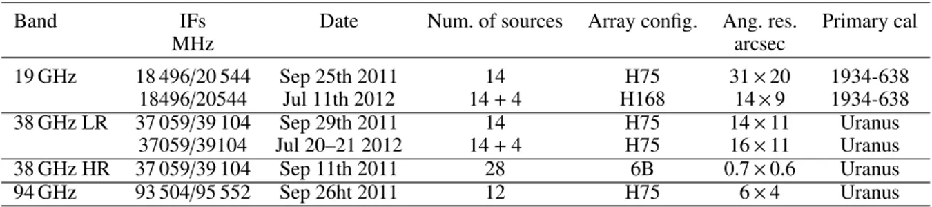
Table 1. Observation details.
Band IFs Date Num. of sources Array config. Ang. res. Primary cal
MHz arcsec 19 GHz 18 496/20 544 Sep 25th 2011 14 H75 31 ⇥ 20 1934-638 18496/20544 Jul 11th 2012 14 + 4 H168 14 ⇥ 9 1934-638 38 GHz LR 37 059/39 104 Sep 29th 2011 14 H75 14 ⇥ 11 Uranus 37059/39104 Jul 20–21 2012 14 + 4 H75 16 ⇥ 11 Uranus 38 GHz HR 37 059/39 104 Sep 11th 2011 28 6B 0.7 ⇥ 0.6 Uranus 94 GHz 93 504/95 552 Sep 26ht 2011 12 H75 6 ⇥ 4 Uranus
Notes. The table lists: dates, number of sources, intermediate frequencies (IFs), array configurations, angular resolutions (ang. res.), primary calibrators used during the 2011–2012 observing campaigns. LR: low angular resolution; HR: high angular resolution.
2.2. Observations
The observations at 19, 38, and 94 GHz with the Australia Tele-scope Compact Array (ATCA) were carried out in two separate campaigns in 2011 and 2012. The total observing time for each target was calculated based on the expected flux density at 38 and 94 GHz. To compute the expected flux density the spectral index between 5 or 8 GHz and 19 GHz from the 2007 and 2008 observations was used. For the two new sources the 1.4–5 GHz spectral index from Paper I was used. In Table 1 the relevant information on the 2011–2012 observing campaign is provided. 2.2.1. Observations at 19 GHz
The 15 mm receiver with simultaneous intermediate frequen-cies (IFs) set at 18 496 and 20 544 MHz and a bandwidth of 2048 MHz for each IF was used for these observations. On September 25, 2011, 14 sources out of the list of 28 targets were observed. A hybrid and very short array configuration was chosen in order to map the sources with the same resolution as for the previous multi-frequency observations (Papers I and III, ⇠10 arcsec). The best array configuration for this purpose is H168 but, for scheduling constraints, we observed with the more compact array H75 which provides an angular resolution that is a factor of two larger than H168. For bandpass calibration we took a single ten-minute scan on 1921-293. A five-minute scan on the primary ATCA calibrator 1934-638 was used to boot-strap the absolute flux density scale and 2223-488 was used as pointing and phase calibrator and observed approximately every 20 min. On July 18, 2012, the remaining 14 sources in our sample, plus four objects which were not detected (signal-to-noise ratio (S/N) < 5) in the 2011 run, were observed with the hybrid array configuration H168. The bandpass calibrator was 1921-293 which was observed in a single seven-minute scan. The absolute flux density calibrator was 1934-638 which was observed in a single five-minute scan. The pointing and phase calibrator was 2223-488.
2.2.2. Low-resolution observations at 38 GHz
The two IFs of the 7-mm receiver were set to frequencies 37 056 and 39 104 MHz with a bandpass of 2048 MHz for each IF. On September 29, 2011, 14 sources were observed with the array in its most compact configuration H75 in order to provide inte-grated flux density measurements for the radio spectra at sim-ilar resolution to the other frequencies. The bright calibrator 1921-293 was used for bandpass corrections, 2223-488 as phase calibrator and the planet Uranus as absolute flux density cali-brator. On July 20 and 21, 2012, the remaining 14 sources were
observed with the most compact array configuration H75. The four undetected objects mentioned above were also reobserved to obtain flux densities at 19 and 38 GHz at the same epoch. The same calibrator setting as for the 2011 observations was used. 2.2.3. High-resolution observations at 38 GHz
On September 10 and 11, 2011, the full sample of 28 sources was observed at 38 GHz with the array configuration 6B in order to achieve the highest angular resolution (0.6 arcsec). The fre-quency setting and bandwidth was the same as that in the low-resolution run. The Hour Angle (HA) coverage spanned the range between 6hand +6hin order to maximize the (u, v)
cov-erage of the linear array configuration. A single scan of 5 min on the strong source 1921-293 was used as band-pass calibra-tion. For absolute flux density calibration the planet Uranus was observed in a single scan for 10 min. The bright calibrator 2223-488 was chosen as pointing and phase calibrator: the pointing was checked approximately every an hour during observations and a one-minute scan on the phase calibration was repeated every 20 min.
2.2.4. Observations at 94 GHz
On September 26, 2011, we observed a list of 12 sources out of the full sample of 28 targets with the 3-mm receivers with two simultaneous IFs centred at 93504 and 95552 MHz and a bandwidth of 2048 MHz for each IF. The 12 sources showed an inverted- or flat spectrum between 8 and 19 GHz from previous ATCA observations in 2007–2008 so they had the highest chance of being detected. The most compact array configuration H75 was chosen in order to avoid losing flux density because of atmo-spheric phase instability. At 94 GHz this configuration provides a resolution of ⇠5 arcsec. A single five-minute scan on 1921-293 was used for bandpass calibration, a ten-minute scan on the planet Uranus provided absolute flux density calibration and three-minute scans every 20 min on 2223-488 provided phase calibration. A pointing check every hour during observations was also done on 2223-488 together with a paddling sequence for system temperature evaluation.
2.3. Data reduction
We used the astronomical software package MIRIAD (Sault et al. 1995) to reduce all the raw visibility data. We imported the data into MIRIAD, then checked, flagged, and split them into single-source single-frequency data sets. To equalise the bandpass we used the standard ATCA calibrator 1921-293
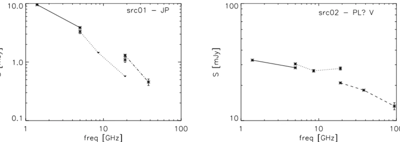
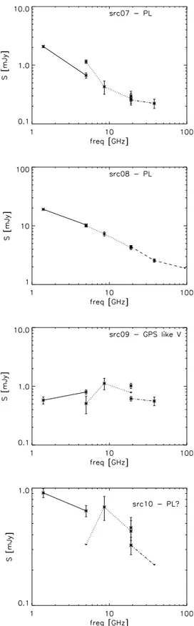
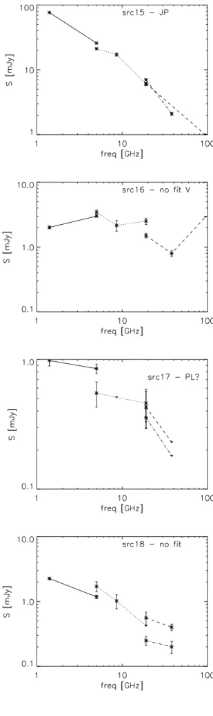
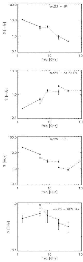
Fig. 1.ATESP sample radio spectra. Asterisks are detections, (with error bars) downward triangles are upper limits, solid lines join ATESP survey points, dotted lines join 2007–2008 follow-up points, dashed lines join 2011 follow-up points, and dot-dashed lines join 2012 follow-up points. for all the runs in 2011 and 2012. The absolute flux density scale
was bootstrapped using the standard ATCA primary calibrator 1934-638 for the 19 GHz (K-band) observations. The planet uranus was instead used for the 38 and 94 GHz observations, because the model of 1934-638 at these bands was too poorly known at that time to perform absolute flux bootstrapping. The phase calibrator 2223-488 was consistently used for all 2011 and 2012 runs to solve for the amplitude and phase complex gains for each observing frequency. The calibrated visibilities were then imaged by Fourier inversion: for the data sets taken with the hybrid and compact arrays H75 and H168, the 6-km antenna data were split away and not reduced because the baselines with the 6-km antenna provide a very poor (u, v) coverage for such configurations. As the bandpass in continuum mode is very large (2 GHz bandwidth) an algorithm available in the package MIRIAD allows for bandpass slope correction over the bandwidth of each IF. For mapping, the Multi Frequency Synthesis (MFS; Sault & Wieringa 1994) technique was used to merge the calibrated visibilities from the two IFs in each observing band (19, 38, and 94 GHz). If the two IFs are not too far apart, the MFS technique can be used to e↵ectively increase the (u, v) plane coverage, minimize the bandwidth smearing and improve the image quality. As we were carrying out a detection experiment the inverted maps were inspected with the visualisation tool kvis of the KARMA software package to search for at least a 3- detection in the map position where a source was expected to be found (the field centre). In case a detection was found the inverted map was cleaned using the task CLEAN in MIRIAD which implements one of the three standard cleaning algorithms (Högbom 1974;Clark 1980;
Steer et al. 1984). When the restored I-Stokes images showed that more than one component was present, a Gaussian fit was performed on those components with the MIRIAD task imfit to determine their flux densities, as well as the integrated flux density of the combined source.
3. Data analysis
3.1. Low-resolution data analysis
In total 26 sources were found to be best fitted by a single-component point-like model at 19 GHz. One source (J225034 401936) appears extended and elongated in the south-west (SW) direction in agreement with what was found in its previous 19 GHz observations (see Paper III) and with its lower-frequency morphology, where two components are clearly seen
along the same direction (see Fig. 7 of Paper III). Finally, one source (J224719 401530) appeared as a double and was fitted with two Gaussian components with integrated flux densities of 0.422 and 0.390 mJy. This source is one of the two not previously observed at 19 GHz.
At 38 GHz 24 sources were best fitted by a single compo-nent point-like model, three sources presented only upper limits, and one source (J225004 402412) was fitted with two Gaus-sian components with integrated flux densities of 0.267 and 0.173 mJy. This source appears as compact at lower frequency, and even in the high-resolution (2 arcsec) 5-GHz images (see Fig. 7 of Paper III). Error bars were computed by summing two terms in quadrature: a multiplicative term related to the residual gain calibration and an additive term related to the root mean square (rms) noise in the V-Stokes maps.
The integrated flux densities with their 1- error bars are listed in Table A.1 in Appendix A together with the orig-inal 1.4-GHz and 5-GHz flux densities from Prandoni et al.
(2000b, 2006). The radio spectra shown in Fig. 1 and Appendix A include all observations available for each source (Prandoni et al. 2000b, 2006,2010). We often have detections and upper limits at the same frequency, coming from di↵erent observing runs with apparently di↵erent quality. We note that there is only one observing run at 94 GHz resulting in only one detection out of 12 objects observed.
3.2. High-resolution data analysis
The 38-GHz I-Stokes images with an angular resolution of 0.6 arcsec were inspected with the KARMA software tool kvis. Only eight sources showed a detection above 3 when the image peaks in the I-Stokes uncleaned maps were compared with the rms noise values in the V-Stokes maps. In 20 cases no bright peak was found in the centre of the map. Seven of the eight detected sources appeared point-like in these high-resolution maps. For the brightest source in the sample (J224547 400324) we self-calibrated the phases in the complex visibilities. This approach produced a structure slightly elongated to the north-west (NW). This source appeared as resolved also at low fre-quency (see Table 5 where the linear sizes of the sources are reported based on 5 GHz imaging with resolutions 2 arcsec, see Paper I for more details). The 38-GHz flux densities (or upper limits) obtained from the analysis of the high-resolution images are also reported in TableA.1.
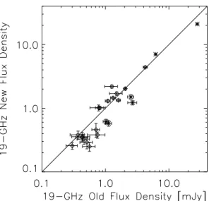
In Fig.2we show high- vs. low-resolution 38-GHz flux den-sities. Apart from the 8 high-resolution detections, 17 sources
Fig. 2.High- vs. low-resolution 38-GHz flux density. Asterisks with error bars are detections at both high and low resolution. Downward triangles show sources with 38-GHz high-resolution upper limits and low-resolution detections. Diamonds are upper limits at both resolu-tions. Sources tagged as variable are also indicated by squares. present an upper limit in their high-resolution flux densities and 3 sources show an upper limit in both high- and low-resolution maps. The strongest sources are detected at both high- and low resolution. All sources are located below or on the one-to-one flux density line meaning that part of the total flux density of the sources is resolved out when imaged at high resolution. The large majority of sources with low-resolution 38-GHz flux density below 1 mJy lose up to 50% of their total flux den-sity when imaged at high resolution, due to structure that is resolved out in high-resolution maps. The three sources with both high- and low-resolution upper limits (diamonds) are clus-tered on the one-to-one line. This is caused by a selection e↵ect: both high- and low-resolution maps have similar detection limits. The seven sources resolved out in their 38-GHz high-resolution maps appeared as resolved also at 5 GHz (see Table5), except for two sources (J225430 400334 and J225529 401101). For these latter sources we can infer an 0.6-arcsec lower limit on their 38-GHz angular size.
An additional technique based on the amplitudes of the vis-ibilities was investigated in order to extract source structure information from the data. This technique was first used by
Chhetri et al. (2013) to detect high-resolution structure in the visibility data of the sources in the AT20G catalogue. This tech-nique consists of taking the ratio of the averages of visibility amplitudes (called gamma factor) for all the baselines with and without antenna CA06 and computing it as a function of HA. The ratio of the averaged amplitudes between long and short baselines in these two sub-arrays provides a clear indication of the presence of structure along certain HAs.
We applied this technique to the 19-GHz dataset only, because the 38-GHz data did not have high-enough S/N (i.e. the error bars in the amplitude ratio were too large) to discriminate a signifi-cant o↵set from the threshold value, the point-like case. In addi-tion, the 19-GHz visibilities are the most resistent to calibration instabilities. To test this technique, the gamma factor was com-puted for the phase calibrator 2223-488 for each scan and IF. The phase calibrator 2223-488 is known to be point-like at the angular resolution sampled by this technique (0.15 arcsec at 19 GHz). A gamma factor of 0.82 corresponds to a single-component Gaus-sian source with a FWHM of 0.15 arcsec. Sources with gamma factor values higher than this threshold are therefore considered point-like for this array configuration. Indeed the gamma factor values of 2223-488 are found to be consistent with the point-like
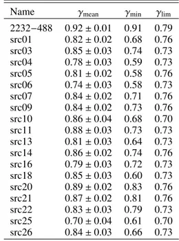
Table 2. Gamma factor statistics at 19 GHz.
Name mean min lim
2232 488 0.92 ± 0.01 0.91 0.79 src01 0.82 ± 0.02 0.68 0.76 src03 0.85 ± 0.03 0.74 0.73 src04 0.78 ± 0.03 0.59 0.73 src05 0.81 ± 0.02 0.58 0.76 src06 0.74 ± 0.03 0.58 0.73 src07 0.84 ± 0.02 0.71 0.76 src09 0.84 ± 0.02 0.73 0.76 src10 0.86 ± 0.04 0.68 0.70 src11 0.88 ± 0.03 0.73 0.73 src13 0.81 ± 0.03 0.64 0.73 src14 0.86 ± 0.02 0.74 0.76 src16 0.79 ± 0.03 0.72 0.73 src18 0.85 ± 0.03 0.60 0.73 src20 0.89 ± 0.02 0.83 0.76 src21 0.87 ± 0.02 0.81 0.76 src22 0.83 ± 0.03 0.79 0.73 src25 0.70 ± 0.04 0.61 0.70 src26 0.84 ± 0.03 0.66 0.73
Notes. Source name, gamma factor mean value with error bar, gamma factor minimum value, and lim: 3 below the gamma factor threshold are given in Cols. 2–4.
case within the error bars. Having found that the gamma factor technique works with our test source (the phase calibrator), we computed the gamma factor for the ATESP sample sources and analysed their values vs. HAs.
In Table2the gamma factor statistics is presented: for each source the mean value is obtained from the average of the gamma factor values over the full range of HAs. For comparison the minimum gamma value ( min) measured within that HA range is
reported together with lim(defined as 0.82–3 , where is the
error associated with gamma mean), that is, the limit below which we consider a source to be significantly resolved. The analysis was performed on the 18 sources that appear point-like on the scatter plot in Fig.2based on the criterion Shigh+3 Slowwhere Slow
is the 38-GHz low-resolution flux density, while Shighand are
the 38-GHz high-resolution flux density and its error bar. Sources with a mean gamma factor value mean < lim at
19 GHz are likely to be extended on sub-arcsec angular scales along several directions. This never happens for our sources.
Comparing the minimum and limit gamma factor values in Table2many sources seem to be resolved in at least one direc-tion (HA), having min < lim. Even if min estimates are less
robust to noise fluctuations and calibration errors, we note that this generally happens for sources known to be resolved from lower frequency – 5 GHz – observations (see Table5). In three cases we measure min < limbut sources appear unresolved at
5 GHz. In such cases (J224827 402515, J224919 400037 and J225436 400531) we can perhaps infer a lower limit to the source sizes of 0.15 arcsec. Source J225322 401931, on the other hand, appears as unresolved at both low and high frequency. For this source we can infer a tighter upper limit of 0.15 arcsec.
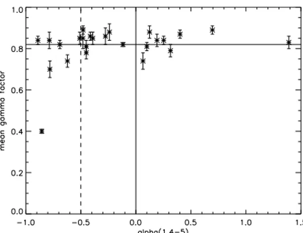
For a more meaningful comparison, the plot in Fig. 3
showing the mean factor vs. the spectral index includes all the ATESP sources and not only those unresolved at 38 GHz.
Chhetri et al.(2013) found a correlation between flat (steep) and compact (extended) sources with extended sources occupying the plot region with ↵5
Fig. 3.Gamma factor vs. ↵5
1.4 spectral index. The vertical dashed and
solid lines indicate ↵ = 0.5 and ↵ = 0, respectively, i.e. the canoni-cal values used to separate steep from flat and flat from inverted spec-trum sources, respectively. The horizontal solid line is the gamma factor threshold for compact sources (angular resolution ✓ < 0.15 arcsec). factor values significantly lower than the threshold. Compact sources are instead grouped around the threshold line indepen-dently of the ↵5
1.4 value. In the ATESP sample most of the
sources belong either to the steep-spectrum compact or the flat/inverted compact classes, with only one object (the double source J225034 401936) clearly in the steep-spectrum/extended part of the plot.
4. Source variability
We have multiple 19-GHz flux density measurements of the ATESP sample. We firstly used the September 2011 and July 2012 observations to determine the two-epoch flux density vari-ability. In case a source was not observed in one of these two epochs or an upper limit was present, the 2007-08 flux densities were used instead. We define as probably variable the sources for which the probability that their flux density is constant over the probed timescale is less than 0.5% and variable the sources for which this probability is less than 0.1%. We obtained this statis-tic via the variability estimator VE = | S/✏c| (Gregorini et al.
1986) where S is the di↵erence between the flux densities at the two epochs and ✏cis the quadratic sum of the flux density errors
at the two epochs. The probably variable sources according to this statistic have a variability estimator value of VE > 2.81, whereas variable sources have VE > 3.29. In cases where a source was tagged as variable or probably variable the strength of its flux density variability was also measured using the esti-mator bySadler et al.(2006):
Vrms =100
hS i qPi(Si hS i)2 Pi 2i.
These results are shown in Table 3 (Cols. 2–4). Figure 4
shows the scatter plot comparing the 19-GHz flux density mea-surements at the two epochs. We found six variable sources (src02, src09, src13, src15, src16, src25) and one probably vari-able source (src24). The probably varivari-able source src02 was also found to be variable in the flux variability analysis presented in Paper III (Prandoni et al. 2010), and src07 and src22 which were tagged as variable in Paper III were not flaring in 2011–2012. For four sources, no variability estimates were possible: src03, src11, src14 and src28.
The results of a 2 test performed on sources with N > 2
epochs at 19 GHz between 2007 and 2012 are also presented in Table3(Cols. 5–7). Three (src06, src13 and src15) of seven
Table 3. 19 GHz variability statistics.
(1) (2) (3) (4) (5) (6) (7) Name VE Tag Vrms 2 P Vrms (%) (%) src01 1.77 src02 8.14(III) V 13.9 src04 2.08 5.62 0.06 src05 1.56 src06 1.09 13.86 9.8e-4 5.0 src07 0.63(III) 0.51 0.77 src08 0.52 src09 3.45 V 22.5 src10 1.16 2.43 0.30 src12 0.56 src13 3.90 V 29.8 54.17 <1e-5 26.5 src15 6.10 V 6.4 124.04 <1e-5 6.1 src16 3.31 V 22.8 src17 0.50 1.11 0.57 src18 2.33 src19 1.64 src20 0.84 src21 1.58 src22 0.15(III) src23 0.99 src24 2.93 P 23.6 src25 3.29 V 33.7 src26 0.10 src27 1.68
Notes. Columns 1–7: source name; two-epoch VE value of (III) means that that source was found to be variable also in the analysis presented in Paper III; variability tag: V for variable, P for probably variable; variability strength associated to two-epoch VE; 2 test for sources
with 19 GHz flux measurements for more than two epochs; associated probability of random fluctations; variability strength for sources with P < 0.1%.
sources with multiple 19-GHz flux densities are classified as vari-able. For these sources there is a probability of less than 0.1% of confusing true variability with statistical fluctuations in flux den-sity. For those three sources the variability strength Vrms is also reported. Only two sources (src13 and src25) show '30% vari-ability over a one-year timescale, that is, 7–8% of the sources. Given the very low sample sizes, this is consistent with the results ofSadler et al.(2006), reporting 5% strongly variable sources at K-band.
Summing together the results obtained from two- and multi-epoch variability analyses we find, however, that a significant fraction (about one third) of our sources show some sign of vari-ability. From the overall spectra shown in Fig.1, we see that at least three variable sources are doubtful: src6, src15 and src25. Indeed all three are very extended (>100 kpc, see Table5) and present relatively smooth steep spectra, that can be fitted by a one or two-component power law (see Sect.6).
5. Model fits of the radio spectra
Inspection of Fig. 1 shows that there are, broadly speak-ing, four categories of radio spectra: (i) smooth-steep spectra, sometimes steepening further at the higher frequencies, (ii) flat spectra, sometimes steepening at the higher frequencies, (iii) peaked spectra, that is, inverted at low frequencies and steep
Fig. 4.Flux–flux scatter plot comparing the 19 GHz flux density mea-surements taken during the 2011–2012 campaign. When one of the two measurements was missing or only an upper limit was available, the 2007–2008 flux density was used instead, if available.
at high frequencies, and (iv) spectra with undefined shape, which may be due to the presence of more than one radio component; in some cases however source variability may be the most likely cause. Some examples are sources src04, 10, 13, and 17 where there are clear jumps for flux densities at the same frequency but observed in di↵erent epochs.
In order to get a more quantitative idea we fitted the spectra with either a power-law (PL) or a Ja↵e-Perola (JP;Ja↵e & Perola 1973) model using the programme Synage (Murgia et al. 1999). We used all detected flux densities and included upper lim-its only when no detection was available at a particular fre-quency. We note that the fitting with a JP model assumes a fixed ↵injection=0.7. For a power-law fit, ↵injectionis a free parameter.
When possible we also added flux densities at 843 MHz using the Sydney University Molonglo Sky Survey (SUMSS;
Mauch et al. 2003) maps. We computed the 843-MHz flux densi-ties directly from the images with the help of the AIPS software. This could be done for 11/28 sources, the remaining being too faint considering the flux limit of SUMSS.
For six sources (src01, src02, src06, src15, src23, src25) there is an entry in the GaLactic and Extragalactic All-sky Murchison Widefield Array (GLEAM;Hurley-Walker et al. 2017) catalogue at 200 MHz. For five of them the 200-MHz point is consistent with the value obtained from the fitting model with-out the GLEAM point and the 2to the fit improves by adding
the GLEAM point. For src01, the flux density of the GLEAM point is higher than the fitting model value and this results in a slightly higher 2 value. From visual inspection of the ATESP
1.4 and 5 GHz images no other confusing source is present in the 2-arcmin beam of the GLEAM survey to justify a spuri-ous flux density increase and the source itself appears point-like. This probably means that the source has di↵use emission at low frequency which is not visible at high frequency.
Four spectra showed signs of steepening at the highest fre-quencies. In those cases we applied a JP model fit. For many other sources a power-law model turned out to provide an appro-priate fit. However, fitting turned out to be impossible for 10 of the 28 sources. For some (three) this is undoubtedly due to vari-ability, but other causes need to be invoked for the remainder: either the sources are of the GPS type (for a definition of GPS, see
O’Dea et al. 1991and also Sect. 6), or have multiple components.
Table 4. Spectral fitting.
Name ↵inj ⌫b(GHz) 2red Comments
src01 0.70 169 3.1 JP src02 0.22 5.5 PL? V src03 0.51 1.4 PL src04 0.59 3.4 PL src05 No fit src06 0.70 110 4.0 JP src07 0.75 4.4 PL src08 0.60 1.5 PL src09 No fit V src10 0.34 0.7 PL?* src11 no fit src12 0.05 3.6 PL src13 no fit; V src14 0.69 6.2 PL** src15 0.70 58 3.6 JP src16 no fit; V src17 0.37 2.0 PL?* src18 No fit src19 0.30 1.1 PL src20 0.70 5.1 PL** src21 No fit src22 No fit src23 0.70 85 1.9 JP src24 No fit; PV src25 1.00 7.0 PL** src26 No fit src27 0.47 2.7 PL?* src28 0.26 1.0 PL
Notes. ↵injis the injection spectral index; ⌫bis the model fit break
fre-quency; 2
redis the reduced 2of the model fit; JP stands for the
Ja↵e-Perola model fit, PL for the power-law model fit. Comments: V(PV) stand for variable (probably variable) spectrum (see Table3); three sources satisfying the variability criteria are not confirmed as such from the inspection of the overall spectra. These sources are src06, src15, and src25. (*) Indicates a slightly more uncertain fit, notwithstanding the low 2value (which is entirely due to the large measurement errors).
(**) Indicates an acceptable fit but the relatively high 2value is due to
the very small formal errors on the flux density.
We note that, looking at the entire spectrum, there are in total seven GPS-like sources, of which two are also variable: src09, src11, src16 (variable), src21, src22, src24 (variable), src26.
We summarise the results of the fitting procedure in Table4. It is worth noting that of the four sources fitted by a JP model, three are extended over more than 100 kpc (see Table 5), and thus represent classical extended radio sources.
The majority of objects that can be fit allow a PL model, but some uncertainty remains; this is indicated by a question mark in Table4.
6. Colour–colour diagrams
A very useful tool for further exploring the spectral behaviour of our sample is o↵ered by colour–colour plots (Sadler et al. 2006) where the spectral index between frequencies in the high-frequency part of the radio source spectrum is plotted against a spectral index in a low-frequency range. This allows the source sample to be split into di↵erent populations based on the radio spectral properties: (i) lower-left quadrant of the plot
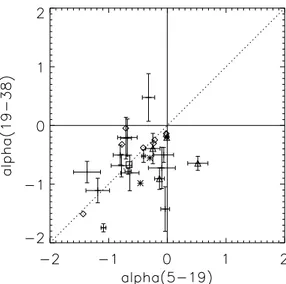
Fig. 5.Colour–colour plot of the ATESP sample with error bars. The triangles are variable sources. Stars are ↵38
19upper limits. Diamonds are
↵19
5 upper limits. Squares represent upper limits in both ↵195 and ↵3819,
while crosses are detections in both axes.
for steep-spectrum sources; (ii) upper-left quadrant for upturn sources, that is, sources which show a trough in their spectrum at a certain frequency; (iii) upper-right quadrant for rising spec-trum sources, and (iv) lower-right quadrant for peaked specspec-trum sources, that is, sources with a radio spectrum peaking in the range of frequencies explored. This last sub-population is typi-cal of GPS-like (GHz-peaked-spectrum) sources (O’Dea 1998). Figure5shows the colour–colour plot of the ATESP early-type source sample with error bars. In this analysis we extended the work done inPrandoni et al. (2010) to 38 GHz. We thus plot-ted the spectral index between 19 and 38 GHz ↵38
19 as ↵high vs.
the spectral index between 5 and 19 GHz ↵19
5 as ↵low (which
was the ↵high in the spectral index analysis of Prandoni et al.
2010). We found that pure ADAF models are still ruled out by the higher-frequency extension of the colour–colour plot, as most of the sources are crowding in the steep-spectrum quad-rant, with just one source (src19) in the upturn quadrant and another one (src24) in the peaked-spectrum quadrant. This lat-ter source is GPS-like by its definition in the colour–colour dia-gram. Other sources that, based on their global spectra, could be classified as GPS-like have their spectral peak at frequen-cies lower than the ones sampled in Fig.5, and therefore do not appear in the peaked spectrum source quadrant. We also notice that a good number of sources are located above the 1:1 line defining single-power-law spectra. Such sources show a flatten-ing goflatten-ing to high frequencies. This flattenflatten-ing is probably asso-ciated to a core component that shows up and dominates at >19 GHz.
We finally investigated the relationship between median spectral index and flux density. To compute the median spec-tral index of the ATESP sample in the presence of upper lim-its we used the Kaplan-Meyer estimator routine inside the Sur-vival analysis package ASURV version 1.2 (Feigelson & Nelson 1985). We found median (mean) values of 0.676 ( 0.619 ± 0.099), 0.650 ( 0.651 ± 0.099) and 0.575 ( 0.510 ± 0.086) for the spectral indices ↵19
5 , ↵3819 and ↵191.4, respectively. In
Fig. 6 we extended the plot of the median spectral index vs. flux density, already presented in Whittam et al. (2013) for the 9C (Waldram et al. 2010) and 10C (AMI Consortium et al. 2011b,a) samples. Here we also include the ATESP sample, the
Bolton et al.(2004) sample, and the Bright and Faint PACO
sam-Fig. 6.Median spectral index as a function of flux density from the ATESP sample (↵19
5 , diamond),Bolton et al.(2004) sample (↵154.8), the
Bright (Massardi et al. 2011) and Faint (Bonavera et al. 2011) PACO samples (↵18
5.5, asterisks). The 9C (triangles) and 10C (squares) survey
points (↵15
1.4) inWhittam et al.(2013) are also shown for comparison.
ples (Massardi et al. 2011;Bonavera et al. 2011). The latter two samples provide information at the bright end of the plot. We confirm the trend already found byWhittam et al.(2013): mov-ing from higher to lower flux-density regimes, radio source spec-tra get steeper and steeper until 10–20 mJy when they turn over to become flat again at the sub-mJy level. The ATESP point gen-tly fits into the general trend shown in the plot. In the ATESP flux density regime (around 1 mJy) the steep-spectrum popula-tion is still dominant, while at fainter fluxes flat-spectrum radio sources take over.
7. Properties of the ATESP early-type sources
Our flux-limited (S > 0.6 mJy) sample of early-type galaxies is fainter than the sample selected bySadler et al.(2014) from the AT20G survey (Murphy et al. 2010). Our sources are distributed over a large redshift range and are also generally more distant than those ofSadler et al. (2014) (characterised by mean z = 0.058).
Intrinsic luminosities at 1.4 and 5 GHz in the rest-frame have been computed making use of the ↵5
1.4spectral index and the
red-shift information. The linear sizes were computed from the source angular sizes obtained from the 2-arcsec-resolution survey maps. Sources with an angular size smaller than the angular resolution appear point-like in the survey maps, so their linear sizes are upper limits. The numerical values are presented in Table5.
How many sources are compact (defined here as those with a linear size smaller than about 30 kpc)? One should note that sources <15 kpc are called FR0 inSadler et al.(2014). Because in our sample most sources are further away, unresolved sources may have sizes which are typically bigger than those discussed by Sadler: 11/28 are <15 kpc; 10/28 have sizes in the range 15–30 kpc, and 7/28 have larger sizes; 3/28 are very large with sizes >100 kpc. In Sadler’s sample 136/201 (68%) are unre-solved and of these 75% are classified as early-type galax-ies. The rest (32%) are FRI- and FRII-type radio sources (Fanaro↵ & Riley 1974). We selected only early-type galaxies; nevertheless the fraction of compact sources is not very di↵er-ent: 75% of our sources are smaller than 30 kpc.
The 20 cm powers of early-type FR0 sources in Sadler go from 1022W Hz 1 to 1026W Hz 1. This has to be compared
with the range spanned by our FR0 sources, 1021.37W Hz–
Table 5. Intrinsic luminosity and linear size. Name z P5 GHz P1.4 GHz ↵51.4 LS W Hz 1 W Hz 1 kpc src01 0.54 24.71 25.10 0.71 120.0 src06 0.44 24.68 25.02 0.62 320.2 src07 0.61 24.17 24.66 0.89 39.9 src15 1.17 26.55 27.02 0.86 110.5 src18 0.03 21.46 21.74 0.51 10.1 src23 0.43 24.48 24.92 0.79 19.6 src25 1.64 26.40 26.83 0.78 196.4 src02 0.19 24.41 24.48 0.12 12.7 src04 0.40 24.22 24.47 0.45 196.3 src08 0.37 24.67 24.93 0.48 18.7 src10 0.35 23.36 23.51 0.28 <9.9b src13 0.61 24.42 24.67 0.45 8.6 src14 0.13 22.83 23.06 0.41 10.9 src17 0.03 21.31 21.37 0.11 9.6 src19 0.59 24.09 24.24 0.26 12.1 src20 0.30 23.44 23.70 0.48 <8.9c src27 1.58 24.99 25.15 0.29 <33.9 src28 0.73 23.32 23.45 0.24 <14.1a src09 1.25 24.35 24.21 0.25 <17.1b src11 0.15 22.63 22.56 0.12 19.9 src12 0.25 23.38 23.34 0.06 4.0 src16 0.03 21.84 21.67 0.31 3.6 src21 0.36 23.33 23.11 0.40 32.7 src22 1.40 24.21 23.44 1.39 5.1 src24 0.56 23.43 23.31 0.70 <12.9a src26 0.44 23.41 23.30 0.19 <11.4b
Notes. Columns 1–6: source name; redshift; rest-frame luminosity at 5 and 1.4 GHz; spectral index used to compute rest-frame luminosity; linear size in kpc. Sources are divided into three groups based on the spectral index: (from top to bottom) steep-, flat-, and inverted-spectrum sources.(a)These sources appear as resolved at 0.6 arcsec resolution. For
these sources we can infer a lower limit in size equal to one third of the quoted values (see Sect.3for more details).(b)These sources appear as
resolved at 0.15 arcsec resolution. For these sources we can infer a lower limit in size equal to one tenth of the quoted values (see Sect.3for more details).(c)This source appears as unresolved down to 0.15 arcsec. This
gives a more stringent size upper limit of <1 kpc (see Sect.3for more details).
The resolved sources (except one) are relatively power-ful, from 1024.47W Hz 1 to 1027.02W Hz 1. We calculated the
equipartition value of their magnetic field, which ranges from a few µG to, for the smallest sources, 10–20 µG. These values are consistent with the normal magnetic field strengths found in early-type radio galaxies.
The large majority of the spectra allowing for a model fit can be represented well by a power-law spectrum, and there is no trace of high-frequency steepening. Therefore such sources will be relatively young. In the four sources fitted with a JP model the break frequencies obtained from the fit give an indication of the source age and this turns out to be around a few million years. One should note that the sources showing steepening are also the most powerful and the biggest sources (of the FRII type), but they are still relatively young with respect to typical radio sources with those sizes.
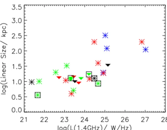
The 1.4 GHz rest-frame luminosities have been plotted against the linear size in Fig. 7. Blue points in the plot rep-resent sources fittable with a JP model, red points are sources
Fig. 7.Rest-frame 1.4 GHz luminosity vs. linear size for the ATESP early-type galaxy sample. Asterisks represent sources with resolved sizes, while downward triangles represent upper limits. The quality of the model fit is colour-coded: blue for JP fits, red for power-law fits, black for uncertain fits (all PL marked with a question mark in Table4) and green for sources that did not permit fitting. The 5 reliably variable sources are inside squares.
following a power-law fit, and black points are uncertain fits, while green points are for non-fittable sources. Radio sources in the linear size (LS) vs. Power plot with larger luminosity (L > 1024.5W Hz 1) have steep or steepening spectra and larger
angular sizes comparable with the ones of B2-type classical radio galaxies. Sources with flat (non-fittable) radio spectra have instead lower luminosity and smaller linear sizes. There is also a class of compact sources that can be fit with a power-law spectra at low luminosity that might be the extension at low power of the linear size-luminosity relation for the B2-type radio galaxies.
In Fig.7sources with upper limits in their linear size have low luminosity; we thus infer that there are three distinct source populations: (i) the bright and large sources representing classi-cal radio galaxies (18%); (ii) compact (confined within their host galaxies), low-luminosity, power-law (jet-dominated) sources (⇠46% of the sample) and (iii) compact, more variable, core-dominated sources (36% of the sample) with linear sizes <30 kpc (thus confined inside their host galaxy), flat radio spectra and a 1.4-GHz luminosity ' 1024W Hz 1 similar to the FR0 sources
classified byBaldi et al.(2016). The ↵5
1.4 spectral index has also been used to separate
the sample into spectral classes: steep-spectrum sources (with ↵51.4 < 0.5, top part of Table 5), flat-spectrum (with 0.5 < ↵51.4 0, middle part of Table 5), and peaked spectrum (with ↵51.4 > 0, bottom part of Table 5). All steep-spectrum sources are resolved at the 2-arcsec angular resolution. Four of eleven flat-spectrum sources and three of the eight peaked spectrum sources have upper limits in their linear size. The rest-frame luminosity vs. linear size plot is compared with the one in Fig. 1 inKunert-Bajraszewska (2016). Most of our resolved sources overlap with the FRI sources (with LS > a few tens of kilopar-sec and L1.4GHz >1024.5W Hz 1) more than the low-luminosity
compact (LLC) sources (with LS between 0.1 and 10 kpc and 1024.5W Hz 1<L
1.4GHz<1026.5W Hz 1). 8. Summary
Here we present quasi-simultaneous observations at 19, 38, and 94 GHz of a sample of 28 early-type radio galaxies carried out in two observing campaigns (September 2011 and July 2012). The main results are summarised below.
All 28 sources were detected in 19 GHz low-resolution maps at 3 level, while 25 sources were detected in 38 GHz low-resolution maps; for three sources we reported 3- flux density upper limits. Only one (src02) of the twelve sources observed was detected at 94 GHz and for the rest of them we report 3- upper limits.
Eight sources were detected at the 3- level in 38 GHz maps at an angular resolution of 0.6 arcsec. Seven sources appear point-like and one source (src02, the brightest one) shows a tentative NW elongation. When comparing low- and high-resolution maps, seven sources have their flux densities resolved out in 38 GHz high-resolution maps. This sets a 0.6 arcsec lower limit on the angular size of the sources unresolved in 5-GHz survey images (Paper I). To the 18 sources appearing as point-like from this anal-ysis we applied a technique based on the ratio of the amplitudes of visibilities (gamma factor) to extract information on source struc-ture down to angular scales of 0.15 arcsec. This analysis shows no clear presence of source structures on the sub-arcsec scale. For the sources unresolved in the images of the 5-GHz survey, this sets a 0.15 arcsec upper-limit (a factor of ten lower).
Six of 25 sources were found variable at 19 GHz with a con-fidence level of more than 99.9% using the two-epoch VE test. These sources are variable in a range between 6.4 and 33.7%. The percentage of variable sources in the ATESP sample turns out to be higher than the 5% found bySadler et al.(2006) on a sub-sample of the AT20G survey.
From the study of the radio spectra, four categories of sources were identified: (i) smooth steep-spectrum sources; (ii) flat-spectrum sources; (iii) peaked-spectrum sources, and (iv) sources having spectra with undefined shape. The spectra of the first kind were fitted with a power law or a JP model. The majority of the sources that could be fit follow a PL model, but for four sources showing signs of spectral steepening at the high-est frequency a JP model fit was applied.
From the analysis of the colour–colour plot, pure ADAF models are still ruled out, as already found in the study at lower frequencies byPrandoni et al.(2010). Twenty-six (93%) sources populate the steep-spectrum quadrant of the plot, while only one source is up-turn and another one has a peaked spectrum. No source is found in the rising spectrum quadrant where sources with an ADAF model are expected to reside.
We computed the median spectral index between 5 and 19 GHz (↵19
5 ) and compared it with data with increasing flux
density threshold from the 9C and 10C surveys (Whittam et al. 2013), the Bolton et al. (2004) sample, and the PACO Faint (Bonavera et al. 2011) and Bright (Massardi et al. 2011) samples. All these points follow a clear trend which the ATESP point is part of: steep-spectrum sources dominate at around 10 mJy, and the flat-spectrum sources increase their contribution toward fainter flux densities. The ATESP sample with a median flux of 1.18 mJy has an intermediate behaviour with a median ↵19
5 ⇠ 0.64.
From the study of the source properties one can con-clude that in the ATESP sample three populations are present: (a) bright and large classical radio sources (18% of the sam-ple) with equipartition magnetic field strengths of the order of a few µG, a luminosity L1.4 GHz> 1024W Hz 1, and linear sizes
>100 kpc; (b) compact (confined within their host galaxies), low-luminosity, power-law (jet-dominated) sources (⇠46% of the sample), and (c) typically flat-spectrum (i.e. non fittable), vari-able, and compact (core-dominated) radio sources (36% of the sample) with linear sizes below 30 kpc (confined inside their host galaxies). This is in agreement with the result found by
Sadler et al.(2014) in a sample of local (z = 0.058) radio sources selected at 20 GHz from the AT20G catalogue.
We conclude that the AGN component of the faint radio pop-ulation appears as a composite ensemble of source types and more accurate studies at higher angular resolution (via VLBI follow-up observations) and higher frequencies (>100 GHz via ALMA) are needed to better characterise it.
Acknowledgements. The Australia Telescope Compact Array is part of the Australia Telescope which is funded by the Commonwealth of Australia for operation as a National Facility managed by CSIRO. We thank Matteo Murgia (INAF-Cagliari), who made available to us his fitting programme SYNAGE.
References
AMI Consortium, Franzen, T. M. O., Davies, M. L., et al. 2011a,MNRAS, 415, 2699
AMI Consortium, Davies, M. L., Franzen, T. M. O., et al. 2011b,MNRAS, 415, 2708
Baldi, R. D., Capetti, A., & Giovannini, G. 2016,Astron. Nachr., 337, 114
Blundell, K. M., Rawlings, S., & Willott, C. J. 1999,AJ, 117, 677
Bolton, R. C., Cotter, G., Pooley, G. G., et al. 2004,MNRAS, 354, 485
Bonavera, L., Massardi, M., Bonaldi, A., et al. 2011,MNRAS, 416, 559
Bonzini, M., Padovani, P., Mainieri, V., et al. 2013,MNRAS, 436, 3759
Chhetri, R., Ekers, R. D., Jones, P. A., & Ricci, R. 2013,MNRAS, 434, 956
Clark, B. G. 1980,A&A, 89, 377
Colla, G., Fanti, C., Fanti, R., et al. 1975,A&AS, 20, 1
Fanaro↵, B. L., & Riley, J. M. 1974,MNRAS, 167, 31P
Feigelson, E. D., & Nelson, P. I. 1985,ApJ, 293, 192
Giroletti, M., Giovannini, G., & Taylor, G. B. 2005,A&A, 441, 89
Gregorini, L., Ficarra, A., & Padrielli, L. 1986,A&A, 168, 25
Högbom, J. A. 1974,A&AS, 15, 417
Hurley-Walker, N., Callingham, J. R., Hancock, P. J., et al. 2017,MNRAS, 464, 1146
Ja↵e, W. J., & Perola, G. C. 1973,A&A, 26, 423
Jones, D. H., Read, M. A., Saunders, W., et al. 2009,MNRAS, 399, 683
Kunert-Bajraszewska, M. 2016,Astron. Nachr., 337, 27
Marriage, T. A., Baptiste Juin, J., Lin, Y.-T., et al. 2011,ApJ, 731, 100
Massardi, M., Ekers, R. D., Murphy, T., et al. 2011,MNRAS, 412, 318
Massardi, M., Bonaldi, A., Bonavera, L., et al. 2016,MNRAS, 455, 3249
Mauch, T., Murphy, T., Buttery, H. J., et al. 2003,MNRAS, 342, 1117
Mignano, A., Prandoni, I., Gregorini, L., et al. 2008,A&A, 477, 459
Murgia, M., Fanti, C., Fanti, R., et al. 1999,A&A, 345, 769
Murphy, T., Sadler, E. M., Ekers, R. D., et al. 2010,MNRAS, 402, 2403
Nagar, N. M., Wilson, A. S., & Falcke, H. 2001,ApJ, 559, L87
O’Dea, C. P. 1998,PASP, 110, 493
O’Dea, C. P., Baum, S. A., & Stanghellini, C. 1991,ApJ, 380, 66
Prandoni, I., Gregorini, L., Parma, P., et al. 2000a,A&AS, 146, 31
Prandoni, I., Gregorini, L., Parma, P., et al. 2000b,A&AS, 146, 41
Prandoni, I., Parma, P., Wieringa, M. H., et al. 2006,A&A, 457, 517
Prandoni, I., de Ruiter, H. R., Ricci, R., et al. 2010,A&A, 510, A42
Quataert, E., & Narayan, R. 1999,ApJ, 520, 298
Sadler, E. M., Ricci, R., Ekers, R. D., et al. 2006,MNRAS, 371, 898
Sadler, E. M., Ekers, R. D., Mahony, E. K., Mauch, T., & Murphy, T. 2014,
MNRAS, 438, 796
Sajina, A., Partridge, B., Evans, T., et al. 2011,ApJ, 732, 45
Sault, R. J., & Wieringa, M. H. 1994,A&AS, 108, 585
Sault, R. J., Teuben, P. J., & Wright, M. C. H. 1995,ASP Conf. Ser., 77, 433
Seymour, N., Dwelly, T., Moss, D., et al. 2008,MNRAS, 386, 1695
Snellen, I. A. G., Schilizzi, R. T., Miley, G. K., et al. 2000,MNRAS, 319, 445
Steer, D. G., Dewdney, P. E., & Ito, M. R. 1984,A&A, 137, 159
Waldram, E. M., Pooley, G. G., Davies, M. L., Grainge, K. J. B., & Scott, P. F. 2010,MNRAS, 404, 1005
Whittam, I. H., Riley, J. M., Green, D. A., et al. 2013, MNRAS, 429, 2080
Whittam, I. H., Riley, J. M., Green, D. A., Jarvis, M. J., & Vaccari, M. 2015,
MNRAS, 453, 4244
Whittam, I. H., Riley, J. M., Green, D. A., & Jarvis, M. J. 2016,MNRAS, 462, 2122
Whittam, I. H., Green, D. A., Jarvis, M. J., & Riley, J. M. 2017,MNRAS, 464, 3357
Appendix A: Radio spectra and flux table
Table A.1. Integrated flux densities of the ATESP sources in the 2011 (Cols. 5–8) and 2012 (Cols. 9–10) campaigns, with error bars.
(1) (2) (3) (4) (5) (6) (7) (8) (9) (10)
1.4GHz 5GHz 19GHz 38GHz LR 38GHz HR 94GHz 19GHz 38 GHz
(mJy) (mJy) (mJy) (mJy) (mJy) (mJy) (mJy) (mJy)
src01 J224516 401807 9.4 3.9 1.091 <0.198 1.297 0.456 0.08 0.08 0.100 0.059 0.058 src02 J224547 400324 32.83 28.28 21.0 18.225 9.4 13.3 0.08 0.08 0.106 0.077 0.092 0.92 src03 J224628 401207 1.35 0.82 <0.32 <0.09 0.323 0.278 0.08 0.08 0.042 0.058 src04 J224654 400107 5.59 3.15 1.602 <0.261 <1.74 1.333 0.829 0.08 0.07 0.117 0.055 0.105 src05 J224719 401530 0.74 0.84 0.812 <0.183 1.015 0.378 0.08 0.07 0.115 0.061 0.097 src06 J224750 400148 13.44 6.09 1.314 <0.297 1.452 0.837 0.08 0.07 0.113 0.057 0.101 src07 J224753 400455 2.08 0.67 0.3 <0.159 0.257 0.223 0.08 0.07 0.060 0.032 0.040 src08 J224822 401808 19.08 10.34 4.408 2.563 1.5 <1.9 0.08 0.07 0.081 0.073 0.090 src09 J224827 402515 0.58 0.80 1.020 <0.27 0.616 0.560 0.08 0.07 0.103 0.056 0.093 src10 J224919 400037 0.91 0.64 0.46 <0.192 0.326 <0.222 0.08 0.07 0.102 0.055 src11 J224935 400816 0.7 0.82 <0.32 <0.294 0.326 0.264 0.08 0.06 0.041 0.032 src12 J224958 395855 1.52 1.65 1.7 1.2 0.87 <1.8 0.09 0.07 0.103 0.077 0.092 src13 J225004 402412 3.16 1.78 1.122 <0.261 <1.3 0.578 0.440 0.09 0.07 0.127 0.058 0.065 src14 J225008 400425 2.88 1.7 0.49 <0.249 0.430 0.416 0.09 0.07 0.141 0.055 0.073 src15 J225034 401936 76.6 25.8 6.165 <0.267 <1.0 7.031 2.100 0.09 0.07 0.130 0.057 0.100 src16 J225057 401522 2.01 3.0 1.5 0.8 0.78 <2.9 0.09 0.06 0.121 0.079 0.084 src17 J225223 401841 0.98 0.85 0.43 <0.228 <0.255 0.356 <0.180 0.09 0.07 0.137 0.060 src18 J225239 401949 2.26 1.18 0.56 0.402 <0.141 0.250 0.200 0.09 0.07 0.127 0.046 0.040 0.041 src19 J225249 401256 1.52 1.09 0.46 0.64 <0.267 <0.93 0.09 0.06 0.115 0.083 src20 J225322 401931 1.86 1.01 <0.35 <0.16 <0.189 0.347 0.198 0.09 0.07 0.042 0.034 src21 J225323 400453 0.51 0.85 <0.35 <0.25 <0.261 <1.5 0.380 0.230 0.09 0.06 0.042 0.050 src22 J225344 401928 0.6 3.52 2.03 1.414 1.2 <3.13 0.09 0.06 0.103 0.077 0.090 src23 J225404 402226 10.34 3.8 1.014 0.47 0.22 0.09 0.06 0.110 0.045 0.050 src24 J225430 400334 <0.26 0.63 2.19 1.4 0.87 <1.4 0.06 0.128 0.082 0.086 src25 J225434 401343 21.09 7.8 1.22 0.860 <0.264 <3.0 0.09 0.06 0.097 0.072 src26 J225436 400531 0.47 0.6 0.37 <0.273 0.381 0.321 0.09 0.06 0.092 0.055 0.075 src27 J225449 400918 1.24 0.86 0.51 <0.186 0.291 <0.183 0.09 0.06 0.115 0.061 src28 J225529 401101 1.48 1.09 0.761 0.585 0.279 0.08 0.06 0.102 0.075 0.093
Notes. Flux densities obtained in the 1.4 and 5-GHz ATESP surveys are also shown for comparison in Cols. 3 and 4. A < sign in front of a flux density measurement means a 3- upper limit. LR and HR are the short forms for low-angular-resolution and high-angular-resolution (0.6 arcsec) flux densities, respectively. Every second line shows the flux-density error bar.