2
Sommario
Il presente lavoro di tesi descrive i risultati del progetto di ricerca sviluppato presso il Laboratorio μTomo della sorgente di luce STAR, parte della Progetto PON Materia presso l'Università della Calabria e presso altre facilities internazionali di luce di sincrotrone. Il progetto ha riguardato lo sviluppo degli strumenti di acquisizione e trattamento dati e in particolare la realizzazione di un pacchetto software completo in linguaggio LabView per il controllo remoto del sistema di microtomografia μTomo. La programmazione è consistita nel controllo dell'insieme stazione sperimentale ovvero dei cinque motori passo-passo e del rilevatore a flat panel necessari per l'allineamento del campione e l'acquisizione delle immagini. La prima indagine tomografica eseguita dalla beamline μTomo è quindi riportata e discussa.
Inoltre, il pacchetto software è stato evoluto per essere integrato nel sistema di controllo di STAR cioè per espletare la funzione di server EPICS e consentire il controllo remoto su piattaforma EPICS allo stesso livello di controllo della sorgente dell’intera sorgente STAR. Sono quindi state eseguite una serie di test di funzionamento della stazione sperimentale che hanno portato a risultati nel campo della scienza dei materiali ed in particolare in quella dei dispositivi a semiconduttore.
Come parte del progetto di ricerca, nel quadro di una collaborazione scientifica con il gruppo di lavoro della linea di luce ID17 dedicata all'imaging biomedico, la biologia e la radioterapia, del Sincrotrone ESRF di Grenoble (F), è stata sviluppata una interfaccia utente grafica per rendere disponibile la tecnica di imaging a contrasto di fase in modalità di propagazione – PBI. Il software sviluppato è stato testato effettuando due esperimenti micro-tomografia a raggi X.
Al fine di una migliore esposizione, questo lavoro di tesi è stato diviso in quattro parti: Capitolo I: Fondamenti teorici, descrizione dei fondamentali sulla microtomografia a raggi X.
Capitolo II: Implementazione hardware, descrizione dettagliata del sistema di acquisizione.
3
Capitolo III: Sviluppo e sperimentazione del pacchetto software di controllo della stazione ed acquisizione dati
Capitolo IV: Risultati e discussione su esperimenti effettuati per verificare le prestazioni dei sistemi di micro-tomografia.
4
Abstract
The present dissertation is intended describing the results of the research project developed at the µTomo Laboratory of the STAR light source, as part of the PON MaTeRiA Project at the University of Calabria.
The project involved making the data acquisition and treatment tools by developing a complete software package in LabView language for remote control of the µTomo microtomography system. The programming consisted of control of the whole experimental station including five stepper motors and a flat panel detector necessary for the sample alignment and image acquisition. The first tomographic investigation performed by the µTomo beamline are reported and discussed.
Furthermore, the software was evolved to be integrated into the STAR control system i.e. to run as an EPICS server in LabView language and permit the remote control on a EPICS platform at the same control level as the STAR source.
As part of the research project, in the framework of a scientific collaboration with the ID17 beamline dedicated to biomedical imaging, radiation biology and radiation therapy, of the ESRF Synchrotron in Grenoble (F), a Graphic User Interface was developed for the implementation of the Propagation-based phase-contrast imaging technique, the software was tested by carrying out two micro-CT experiments.
For the sake of a clear description this dissertation was divided into four parts:
Chapter I: Theoretical foundation, description of fundamentals on X-ray microtomography.
Chapter II: Hardware Implementation, detailed description of acquisition system. Chapter III: Development and testing of Data Acquisition Software
Chapter IV: Results and Discussion on benchmark experiments carried out to verify the micro-tomography systems performance.
5
DEDICATION
6 INDEX
1. Theoretical Foundation ... 15
Evolution of X-ray Microtomography ... 15
Introduction to Microtomography ... 16
Phase Contrast in Microtomography ... 21
The noise in microtomography ... 23
The artefacts in microtomography ... 24
Cone Beam in microtomography ... 26
Physical factors which affect the performance of CBCT ... 26
Reconstruction in microtomography ... 28
2. Hardware System ... 34
Microtomography System ... 34
Acquisition in Microtomography ... 36
Syrmep Beamline - Elettra Sincrotrone Trieste ... 36
ID17 – Beamline - ESRF Grenoble ... 39
STAR Facility ... 39
µTomo Laboratory at STAR ... 40
Hardware Beamline Syrmep for acquisition ... 46
3. Software Development ... 49
The Main Program ... 49
3.1.1.Control Motors ... 50
3.1.2. TCP/IP Acquisition ... 55
3.1.3.Subprograms Link ... 57
Upgraded to EPICS I/O Server ... 58
Alternative Software for image acquisition – SYRMEP beamline @ Elettra ... 60
Development of Graphic User Interface (GUI) in Python Language – ID17 beamline @ ESRF ... 61
7
4. Results and Discussion ... 67
Experiment 1: Non-destructive Measurements of Single Events Induced on Power MOSFETs by Terrestrial Neutrons... 67
4.1.1. Introduction ... 67
4.1.2. Materials and methods ... 68
4.1.3. Discussion ... 102
Additional Experiments ... 104
4.2.1. Experiment 2: µ-CT Phase contrast and phase retrieval on organic matter ... 104
4.2.2. Experiment 3: µ-CT Contrast analysis using a phantom ... 110
4.2.3. Experiment 4: µ-CT on a plasticized rat ... 118
4.2.3.1. Introduction ... 118
4.2.3.2. Results: 3D Rendering and Segmentation ... 120
5. Conclusions ... 124
6. Annexes ...126
Annex 1... 126
Annex 2... 127
8 List of Figures
Figure 1: Microtomography - Timeline ... 15
Figure 2: Projection and scanning of the object in plane (t, s) ... 18
Figure 3: Scanning of a single layer in the plane (x, y) ... 18
Figure 4: Attenuation mechanism ... 19
Figure 5: Lambert–Beer Law in homogeneous object ... 19
Figure 6: Lambert–Beer Law in non-homogeneous object ... 20
Figure 7: Projection of sphere phantom in phase-contrast imaging ... 22
Figure 8: Typical Poisson noise ... 23
Figure 9: The artefacts in of sinogram. ... 24
Figure 10: Central slice of a perfect phantom. ... 25
Figure 11: Cone beam CT geometry. ... 26
Figure 12: Cone beam - microtomography system ... 27
Figure 13: Cone beam magnification ... 27
Figure 14: Projection of a slice under parallel object beams ... 29
Figure 15: Generation of a sinogram ... 29
Figure 16: Propagation through of object with different levels of intensity ... 30
Figure 17: Basic back-projected and reconstructed volume ... 30
Figure 18: Typical cone beam micro-CT machine ... 34
Figure 19: Difference between microfocus-CT systems and synchrotron system ... 35
Figure 20: Position of detector respect of magnification ratio. ... 36
Figure 21: Schematic illustration of X-ray CT acquisition and reconstruction processes. 36 Figure 22: Syrmep Beamline ... 38
Figure 23: ID 17- Schematic description of the imaging setup. ... 39
Figure 24: STAR Facility ... 40
Figure 25: Reference of motors ... 41
Figure 26: Experimental Station - µTomo ... 44
Figure 27: Connection diagram ... 45
9
Figure 29: EPICS - Connection Diagram ... 46
Figure 30: SYRMEP setup for acquisition ... 47
Figure 31: Front Panel ... 50
Figure 32: Block Diagram ... 50
Figure 33: Absolute movement - Axis 1 ... 51
Figure 34: Absolute movement - Axis 3 ... 51
Figure 35: Relative movement ... 52
Figure 36: Control rotation, x and y movements ... 53
Figure 37: Hydra – View file ... 54
Figure 38: Absolute movement for rotator ... 55
Figure 39: Front Panel - TCP/IP Acquisition ... 56
Figure 40: File Parameters ... 56
Figure 41: Block diagram – Acquisition ... 57
Figure 42: Block diagram. Link between Subprograms and Main Program ... 57
Figure 43: Front Panel – Epics Server ... 58
Figure 44: Part of block diagram – Epics Server ... 59
Figure 45: Epics Server – LabVIEW Project ... 59
Figure 46: Monitoring Epics Process Variables with Distributed System Manager ... 60
Figure 47: Alternative Software for acquisition image ... 61
Figure 48: Template of Basic Parameters ... 62
Figure 49: Template of Expert Parameters ... 62
Figure 50: Template of Range Parameters ... 63
Figure 51: a) Model for SEB (92); b) and for SEGR (93). ... 68
Figure 52: Detail of neutron irradiate Power MOSFET ... 69
Figure 53: SEM single device – Power MOSFET ... 70
Figure 54: SEM of metal heatsink ... 71
Figure 55: SEM of Si substrate ... 71
Figure 56: SEM of external package ... 71
10
Figure 58: 3D Power MOSFET result of horizontal position ... 74
Figure 59: Vertical scan – Power MOSFET ... 75
Figure 60: Orthogonal cut of the reconstructed MOSFET 3D image by means of a “Vertical scan”. ... 75
Figure 61: MDmesh Power MOSFET Structure ... 77
Figure 62: Power MOSFET volume rendering ... 78
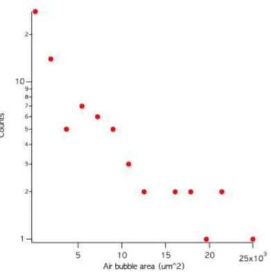
Figure 63: Histogram of the voids area in the Pb layer for the sample MOSFET #1. ... 78
Figure 64: Zoom - Orthogonal View ... 79
Figure 65: Zoom - Orthogonal View and 3D of ROI of interest ... 80
Figure 66: MOSFET #3 - XZ plane cut along the Pb layer ... 80
Figure 67: Zoom on the ROI (Orthogonal View) ... 81
Figure 68: ROI Rendering 3D – Side view ... 81
Figure 69: 2D Projection ... 82
Figure 70: 2D Projection ... 82
Figure 71: 2D Projection ... 82
Figure 72: Side View and zoom view to 150%. ... 83
Figure 73: 2D Projection ... 84
Figure 74: ROI Rendering 3D – Top view ... 84
Figure 75: 3D - Side View and 300% 3D Zoom ... 85
Figure 76: 2D Projection ... 86
Figure 77: Zoom XZ view ... 86
Figure 78: 3D – Side -view ... 87
Figure 79: 3D - Side view and 1200% zoom view. ... 87
Figure 80: 2D µCT cut of MOSFET #1 after n-irradiation ... 88
Figure 81: ROI Rendering 3D – Top view ... 89
Figure 82: 3D Rendering: (a) side view ... 90
Figure 83: 2D µCT cut of MOSFET #2 after n-irradiation ... 91
Figure 84: Orthogonal View and located of damage single device MOSFET #2 ... 91
Figure 85: (a) ROI Rendering 3D – Top view; (b) Perspective view ... 92
11
Figure 87: 2D µCT cut of MOSFET #3 after n-irradiation ... 93
Figure 88: 3D Single Device ROI – Top view and Side view ... 93
Figure 89: 2D µCT cut of MOSFET #4 after n-irradiation ... 94
Figure 90: Orthogonal View across the ROI where the defects is located in MOSFET#4 ..94
Figure 91: MOSFET #4 - 3D Rendering of the ROI:. ... 95
Figure 92: 2D µCT cut of MOSFET #5 after n-irradiation ... 95
Figure 93: n-irradiated MOSFET #5 - Zoom XZ view of the ROI ... 96
Figure 94: n-irradiated MOSFET #5 - 3D.. ... 96
Figure 95: Orthogonal cuts of the 3D µCT reconstruction.. ... 97
Figure 96: Zoom on the ROI- Orthogonal View and 3D of the Pb tab. ... 98
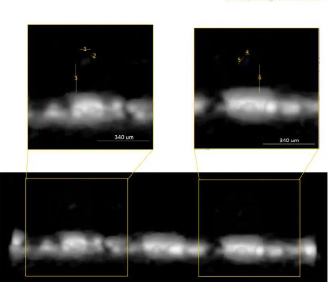
Figure 97: ROI 3D Rendering– Side view. Length 1: 83 µm - length 2: 62 µm. ... 98
Figure 98: 2D µCT cut of MOSFET #7 after n-irradiation ... 99
Figure 99: n-irradiated MOSFET #7 Zoom on the ROI - Orthogonal View and 3D ... 99
Figure 100: ROI Rendering 3D – Side view. Length 1: 54 µm – length 2: 135 µm. ... 100
Figure 101: Typical reconstructed volume slab of the Power MOSFET ... 100
Figure 102: Cross section for 28Si(n,p) 28Al reaction (left) and for 28Si(n, alpha) 25Mg reaction (right - from ENDF/B-VII.1 database) ... 103
Figure 103: Setup of onion specimen ... 105
Figure 104: Cropping normalized projection ... 106
Figure 105: Sinogram of the Onion Bulb, Projection 91. Left: Sinogram. Right: Profile ... 106
Figure 106: Slice 91 reconstruction without phase retrieval ... 107
Figure 107: Slice 91 reconstruction with phase retrieval ... 108
Figure 108: Comparison of the central part of slice 91 reconstructed images. ... 108
Figure 109: 3D Rendering - Filaments ... 109
Figure 110: Phantom placed on the Computed Tomographic stage during the acquisition. . 111
Figure 111: Slice 1000 reconstructed. ... 113
Figure 112: CNR values for phantom materials (above).. ... 116
Figure 113: Plot of CTF ... 117
Figure 114: Plastirat sample on the Computed Tomographic stage. ... 119
12
Figure 116: Segmentation images ... 121
Figure 117: 3D - Transversal view ... 122
Figure 118: Brain - Top View ... 122
Figure 119: Brain - Side View ... 123
13 Acronyms and Abbreviations
µTomo Micro-Tomography
CBCT Cone beam computed tomography
CNR Contrast to noise ratio
COR Center of rotation
CT Computed Tomography
EPICS Experimental Physics and Industrial Control System
ESRF European Synchrotron Radiation Facility
FOD Focus Object Distance
FOV Field of view
GUI Graphic Interface User
LabVIEW Laboratory Virtual Instrument Engineering Workbench
MaTeRiA Materiali, Tecnologie e Ricerca Avanzata
MOSFET Metal-oxide-semiconductor field-effect transistor
micro-CT micro Computed Tomography
NIST National Institute of Standards and Technology
PBI Propagation-based phase-contrast imaging
PON National Operational Program
ROI Region of interest
SDD Source to detector distance
SEEs Single Events
SEB Single Event Burnout
SEGR Single Event Gate Rupture
SOD Source to object distance
SRμCT Synchrotron radiation micro-computed tomography
STAR South Europe Thomson source for Applied Research
STP SYRMEP Tomo Project
SYRMEP Synchrotron Radiation for MEdical Physics
14
Chapter I
Theoretical Foundation
15
1. Theoretical Foundation
Evolution of X-ray Microtomography
The theoretical basis of microtomography has its origins in the year 1917, only few years after that Roentgen discovered X-ray in 1895, when the Austrian mathematician Johan Radon proved that an n-dimensional object can be reconstructed from its n-1 dimensional projections. However, only in the second half of the past century, the mathematical basis for the actual CT image reconstruction was presented in two scientific articles by Allan M. Cormack (See Figure 1).
Figure 1: Microtomography - Timeline
The development of microtomography laboratories emerged in the mid-1960s, creating images by exploiting the X-ray refraction in addition to their absorption. (1)
Nowadays, the X-ray microtomography or micro-computed tomography (micro-CT) is a technique of radiographic imaging able to produce 3D images of the inner structure of a material with a spatial resolution in the order of the micrometers (2).
The first microtomography system was produced by Jim Elliott in the early 1980s. The first microtomographic images were slices of a small snail, with an effective pixel size of
16
approximately 50 micrometers (3).
The first conical scanner was constructed by Feldkamp for the reconstruction of the three-dimensional microstructure of trabecular bone (4).
In 1992, by using the high quality of the radiation emitted by the third-generation synchrotron a resolution of 1-μm was achieved (5). In 1994, with the first commercially available micro-CT scanner, the microtomography technique started to become a standard in bone research. Currently, in-vivo and in-vitro micro-CT scanners are available from several manufacturers (6). The phase contrast imaging, a new technique based on the interfering paths of coherent X-ray beams, will surely continue to expand the applications for micro-CT in small animal models (7).
Laboratory-based micro-CT and nano-CT scanners as well as integrated micro-CT/SPECT and micro-CT/PET scanners are marketed nowadays (8).
Introduction to Microtomography
Microtomography is a non-destructive technique tool that obtains tri-dimensional images exploiting a set of bi-dimensional images from a sample (9).
The principle of micro-CT is based on the attenuation of X-rays passing through the object or sample being imaged. As an X-ray passes through a homogeneous medium, the intensity of the incident X-ray beam is reduced according to the Lambert-Beer equation, Ix = I0 e−μx, where I0 is the intensity of the incident beam, x is the distance covered by the X-ray in the absorbing medium, Ix is the intensity of the beam in the position x from the surface, and μ is the linear attenuation coefficient (10).
Moving to a more detailed description, the X-ray as an electromagnetic wave is characterized by amplitude, polarization, frequency, wave-vector and phase. As a result of the interaction of the electro-magnetic wave with a given medium, its amplitude attenuated, and its phase shifted. The refraction index of any material can be expressed by a complex number (11) (12):
17
The symbol 𝛿 is the refractive index, which determines the phase shift and 𝛽 absorption index of x-ray wave and is expressed by (13):
𝜹 = 𝝀
𝟐𝝅∑ 𝑵𝒌 𝒌𝝓𝒌 Eq. 2
𝜷 = 𝝀
𝟒𝝅∑ 𝑵𝒌 𝒌𝝁𝒌 Eq. 3 where, for each element k,
𝜙𝑘 : phase shift cross-section.
𝜇𝑘 : atomic absorption cross-section. 𝑁𝑘 : atomic density.
The form of the X-ray wave through a uniform medium is (11) - (12):
𝝍(𝒓⃑ ) = 𝑨 ⋅ 𝐞𝐱𝐩(𝒋𝒏𝒌 ⋅⃑⃑⃑⃑ 𝒓⃑ ) = 𝑨 ⋅ 𝐞𝐱𝐩 (−𝜷(𝒌 ⋅⃑⃑⃑⃑ 𝒓⃑ )) ⋅ 𝐞𝐱𝐩(𝒋𝒌 ∙⃑⃑⃑⃑ 𝒓⃑ ) ⋅ 𝐞𝐱𝐩 (−𝜹(𝒋𝒌⃑⃑ ⋅ 𝒓))⃑⃑⃑⃑⃑⃑ Eq. 4
With:
A: initial amplitude 𝑘
⃑⃑⃑⃑ : wave vector
𝑟 ∶ the position vector
From Eq. 4, 𝛽 contributes to the attenuation of amplitude and 𝛿 to the wave phase shift. Theoretically and experimentally it had been demonstrated that, in the X-ray range, 𝛿 is thousands of times larger than 𝛽.
Projections acquisition.
In referring to the projection and scanning of an object, as depicted in Figure 2, we consider the rotation about the z-axis in a rotational coordinate system {s, t, z}. The intensity of the
18
transmitted beam is recorded as a translation function of the position parameter t for each z value. Lambert’s Law gives the transmitted intensity by the following expression: (14)
𝑰(𝒙, 𝒚) = 𝑰𝒐𝐞𝐱𝐩 (− ∫𝒑𝒂𝒕𝒉𝝁(𝒙, 𝒚) 𝒅𝒔) Eq. 5
Figure 2: Projection and scanning of the object in plane (t, s)
Figure 3 indicates the scanning of a single layer in the plane (x, y). Such a projection can be defined by: (14)
𝑷𝜽(𝒕) = 𝐥𝐧 (𝑰𝑰
𝟎) = ∫𝒑𝒂𝒕𝒉𝝁(𝒙, 𝒚) 𝒅𝒔 Eq. 6
19
The attenuation is determined by the sample composition and by the spectral distribution of the X-radiation and can be used to quantify the density of the imaged object. Generally, to obtain such information, the reduced intensity beams are collected by a flat-panel detector (See Figure 4) (9) (15).
Figure 4: Attenuation mechanism
As an example, if we consider a monochromatic ray penetrating through a homogeneous object, the ray attenuation can be explained by the Lambert–Beer Law and depends only on the object thickness x for each point of the projection (see Figure 5) (16) (17) (18).
Figure 5: Lambert–Beer Law in homogeneous object
Figure 6 illustrates two projections acquired for an elliptical test object immersed in a medium with different absorption coefficient (non-homogeneous material). The intensity curve will be related to the geometrical shape of the test object. By following its evolution on the projection angle, it will be possible to reconstruct the whole object shape.
On the right of Figure 6, we find a schematic representation of a more complex situation where two projections acquired from an object consisting of a 2 × 2 matrix of different materials. The intensities of the projections can be expressed in terms of the linear attenuation coefficients by: (19)
𝑰𝟏= 𝑰𝟎𝒆−(𝝁𝟏+𝝁𝟐)𝒙 Eq. 7
20
𝑰𝟑= 𝑰𝟎𝒆−(𝝁𝟏+𝝁𝟑)𝒙 Eq. 9
𝑰𝟒 = 𝑰𝟎𝒆−(𝝁𝟐+𝝁𝟒)𝒙 Eq. 10
Figure 6: Lambert–Beer Law in non-homogeneous object
As already noted, the mathematical bases for the tomographic images were formulated by Johann Radon. Even though it is applied in computed tomography to obtain cross-sectional images of patients, tomographic reconstruction applies for all types of tomography. Some terms or physical descriptions we will use refer directly to computerized axial tomography.
We already showed how the projections of an object at a certain angle θ they are made up of a series of line integrals. In X-ray computed axial tomography, the line integrals represent the total attenuation of the X-ray beam while they travel in a straight line through the object and the resulting image is a 2D (or 3D) model of the absorption coefficient i.e. the image μ(x,y). The simplest and easiest way to visualize the method of analysis is the system of parallel projections. For this we consider the information that is collected as a series of parallel rays in the position r, through a projection in the angle θ. This is repeated for several angles. As the attenuation occurs exponentially in the medium the total attenuation p of lightning in position
r with a projection on the angle θ, is given by the following integral:
Eq. 11
Using the coordinate system of the figure, the value of r, on the point (x, y), will be projected in the angle θ shown by the following equation: x cosθ + y sinθ = r. With this, we see that the equation shown above can be rewritten as follows:
21
Eq. 12
where f (x, y) represents μ (x, y). This function is known as the Radon transform (or sinogram) of the object in 2D resolution. The Fourier section theorem tells us that if we have an infinite number of one-dimensional projections of an object obtained from an infinite number of angles, we can perfectly reconstruct the original object, f (x, y). So, to obtain again f (x, y) from the previous equation we must find the inverse Radon transform. However, the inverse Radon transform has proved to be very unstable with respect to noisy data. In practice, a stabilized and discrete version of the Radon inverse transform is used, which is commonly known as the filtered back-projection algorithm.
Knowing the Radon transform of an object allows it to reconstruct its structure: the projection theoremactually ensures that if we have an infinite number of mono-dimensional projections of an object made from an infinite number of different angles and the reconstruction process is precise when calculating Radon's anti-transformation.
However, Radon's anti-transformation is very unstable if measured data are affected by experimental noise. In practice, a stabilized and discrete version of Radon's anti-transformation, called 'filtered retroprojection algorithm', is used. A corollary to the projection theorem states that "Radon's transformation of the two-dimensional convolution of two functions is equal to
the one-dimensional convolution of their Radon transformations". The practical consequence
of this is that in order to eliminate the noise that reduces the quality of the reconstruction, it is not necessary to physically eliminate it at source, but it is possible to filter mathematically the experimental results (i.e. the measure of the Radon transform) and then rebuild (i.e. calculate the anti-transform) directly from the a posteriori filtered data.
Phase Contrast in Microtomography
Conventionally computed tomography uses the absorption contrast which does not permit some details to be resolved in samples with a weak absorption contrast. In these cases, phase shift of the X-ray beam induced by the variation of the refractive index can be exploited for obtaining
22
a better image (20). A significant improvement over conventional attenuation-based X-ray imaging, which lacks contrast in small objects and soft biological tissues, is then obtained by introducing phase-contrast imaging (21).
The in-line phase-contrast X-ray imaging method, sometimes also called the propagation-based imaging or the inline holography, exploits the Fresnel diffraction and dubbed phase-contrast imaging method in microtomography is possible using the third generation of synchrotron radiation sources or micro-focussed X-ray tube (20) (22).
Thus, as absorption-contrast X-ray imaging serves to visualize the variation in X-ray attenuation within the volume of a given sample, the phase contrast allows us to visualize variations in the X-ray refractive index of the probed volumes (23).
Figure 7 shows the principle of in-line phase-contrast imaging: the projected images of the spheres phantom are shown for different positions of the detector along the z-axis. If z = 0 we have only absorption contrast. The phase contrast occurs in the Fresnel diffraction region, it means that it is necessary to place the detector at a distance from the object where z=d2/ with d the object typical dimension and the X-ray wavelength (20).
Figure 7: Projection of sphere phantom in phase-contrast imaging
The image is edge-enhanced, and for soft tissues, it is possible to retrieve the phase projection from a single in-line image. The phase contrast technique is used for reconstructing the phase coefficient using the retrieved phase projections (24).
In the propagation-based phase contrast X-ray imaging, the contrast effect increases linearly with the sample to detector distance and are given by the equation (25):
23 𝑰(𝒙, 𝒚) = 𝟏 −𝝀𝒛
𝟐𝝅𝛁𝝓(𝒙, 𝒚) Eq. 13 With,
φ(x, y): phase change due to a small slab of material λ: wavelength
z: distance from the sample to the detector
The noise in microtomography
Poisson noise is due to the statistical error of low photon counts, and results in random thin bright and dark streaks that appear preferentially in the direction of greatest attenuation. As the noise increases, high contrast objects such as bone may still be visible, but low contrast soft tissue boundaries may be obscured. Figure 8 illustrates the effect of the increase of the beam intensity on the Poisson noise. Figure 8(A) reproduces an image obtained with a low dose (source current = 60 mA) and shows a series of streaks covering the field of view. Figure 8(B) indicates the image obtained with a higher dose (source current = 440 mA). As the intensity increases by a factor 7.3 the noise is reduced by a factor √7.3 = 2.7. (28)
24 The artefacts in microtomography
The image artefact may be defined as a visualized structure in the reconstructed data that is not present in the object under investigation. Artefacts cause general inconsistencies in the reconstructions (29).
The ring artefact is caused by uncorrected variations in detector dark current, gain, linearity, and defects. Because an erroneous signal is coming from a fixed location on the detector, it produces a linear defect in the sinogram and it is reinforced in back projection at a fixed radius in the reconstruction, that is, on a circle (30). Figure 9 (a) illustrates the sinogram of a crane fly knee, taken from 400 projections over 180°. Several vertical artefacts owing to dead pixels in the CCD corrupt the sinogram. Figure 9(b) depicts the same sinogram after filtering with a one-dimensional low-pass filter. The vertical line artefacts are suppressed without significant loss of information in the sinogram. Figure 9(c) depicts the reconstructed cross-section from the sinogram. Figure 9(a) depicts strong degeneration by half-ring artefacts, and Figure 9(d) depicts how the reconstruction from the filtered sinogram improves the image quality significantly (31).
Figure 9: The artefacts in of sinogram.
(a) Without filter. (b) With filter. (c) Artefacts in the reconstructed cross-section without filter (d) with filter
Figure 10(a) illustrates a central slice of a phantom and its reconstruction with 801 projections. Figure 10(b) depicts the ring artefacts due to variation in detector element sensitivities.
Streak artefacts in reconstructed CT slices can be caused by asymmetric high-density objects (like bones) when low-dose data acquisition is performed, and we cannot correctly recover the
25
line integral. Other possible causes are object motion or/and absorbing particles are made worse misalignment in the scanner geometry description, beam hardening and scatter effects. And finally, streaks can be the result of angular under-sampling, aggravated by missing projections (33). Figure 10(c) depicts streak artefacts due to angular under-sampling in line with straight edges with 401 projections.
If the center of rotation is incorrectly determined, a double-edged image may be seen, Figure 10(d) depicts double edges caused by a 5-pixel error in the value for the center of rotation used in the reconstruction. Meanwhile superficially similar in appearance to images with motion artefacts Figure 10(e) depicts double edges and streaking caused by specimen motion of 10-pixels.
An X-ray beam is composed of individual photons with a range of energies. As the beam passes through an object, it becomes “harder,” its mean energy increases because the lower energy photons are absorbed more rapidly than the higher-energy photons (34). Figure 10(f) depicts the beam hardening artefact caused by polychromatic radiation (34).
Figure 10: Central slice of a perfect phantom.
(a) With 801 projections. (b) Artefacts owing to a detector. (c) 401 projections with streak artefacts. (d) Double edges (e) double edges and streaking. (f) Beam hardening artefact
26 Cone Beam in microtomography
Micro-focal CT (microtomography) in cone-beam geometry is advantageous for obtaining directly reconstructed 3D images from a set of 2D projection images recorded by the detector (35) (36).
Figure 11 illustrates the cone beam CT geometry, it is convenient to assume that the X-ray source and detector system are stationary and that the object rotates around the rotation center (37). Figure 11(a) depicts the setup for filtered image acquisition. Figure 11(b) depicts a top view of the setup. For filtered image acquisition a collimator permits focusing of the FOV (field of view) in the X-ray beam geometry. The ROI (region of interest) filter permits focusing the region of interest in the phantom (38).
Figure 11: Cone beam CT geometry.
(a) Setup for filtered image acquisition. (b) Top view of the setup
Physical factors which affect the performance of CBCT
The main physical factors that affect the performance of CBCT (cone beam computed tomography) is system geometry which allows finding the suitable distances, such as SOD (source to object distance) and SDD (source to detector distance), for reducing the scatter artefacts but maintaining high signal-to-noise ratio (see Figure 12) (30) (39).
27
Figure 12: Cone beam - microtomography system
The focal spot size affects the spatial resolution, particularly for systems with higher magnification, a smaller the value of FOD means the object is near to the focal spot allowing the highest magnification (see Figure 13) (30) (40).
Figure 13: Cone beam magnification
The field of view (FOV) affects a loss in contrast and increases the artefacts (30). There are methods for reducing noise and artefacts that may enable ultra-high resolution limited-field-of-view imaging (28).
The dynamic range we can define simply by the ratio of the maximum and the minimum detectable signal, measured in the gray level or it can also refer to an effective number of bits
28
in the detector. The dynamic range of the acquisition system is the relevant quantity which determines the maximum material thickness which can be inspected (41). Maintaining fixed the FOV while the size of the object increases then noise, contrast, and artefacts increase (30). In micro-focussed sources, the polychromatic beams produced by higher electron acceleration reduce the contrast and increases the noise. On the other hand, a softer beam with a broader spectrum increases the artefacts (30).
Microtomography reconstruction from a limited number of projections provides a method to simultaneously reduce the radiation dose and in many cases the acquisition time (42).
Reconstruction in microtomography
The reconstruction algorithms introduced in paragraph 1.2 can be implemented by using the fast Fourier transform (43).
For a good quality reconstruction, the sample must be rotated through at least 180° (plus the cone angle in CBCT). Datasets are acquired over this angular range with a certain step-size between images (44).
The reconstruction process transforms the raw acquisition data into a stack of 2D cross-sections through the sample, resulting in a 3D data set. Several artefacts and noise reduction algorithms are integrated to reduce ring artefacts, beam hardening artefacts, COR (center of rotation) misalignment, detector or stage tilt, pixel non-linearities, etc (45) .
The parameter of interest in the slice is represented by a 2D function f(x, y), and each projection datum g(u, θ) is a line integral. The equations correspond to u = x cos θ + y sin θ and v = −x sin θ + y cos θ (see Figure 14) (46).
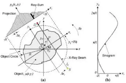
Figure 15 shows (a) schematic arrangement of first generation CT set-up indicating the way projections are built up from a ray-sums. In every projection, a point (P) in the object contributes to one ray-sum along the path from the source (S) to the detector (D). The axes x, and y represent the laboratory frame; xr, yr the rotating frame of the specimen/object. (b) The sinogram of a point P in (a) in the 2-D space (xr ,ϕ) (47).
29
Figure 14: Projection of a slice under parallel object beams
Figure 15: Generation of a sinogram
1.9
.
X-ray Phase retrieval in MicrotomographyPhase retrieval is a method for reconstructing phase from the measured intensity, in-line phase-contrast X-ray imaging provides images where both absorption and refraction contribute. For quantitative analysis of these images, the phase needs to be retrieved numerically (see Figure 16) (48).
30
Figure 16: Propagation through of object with different levels of intensity
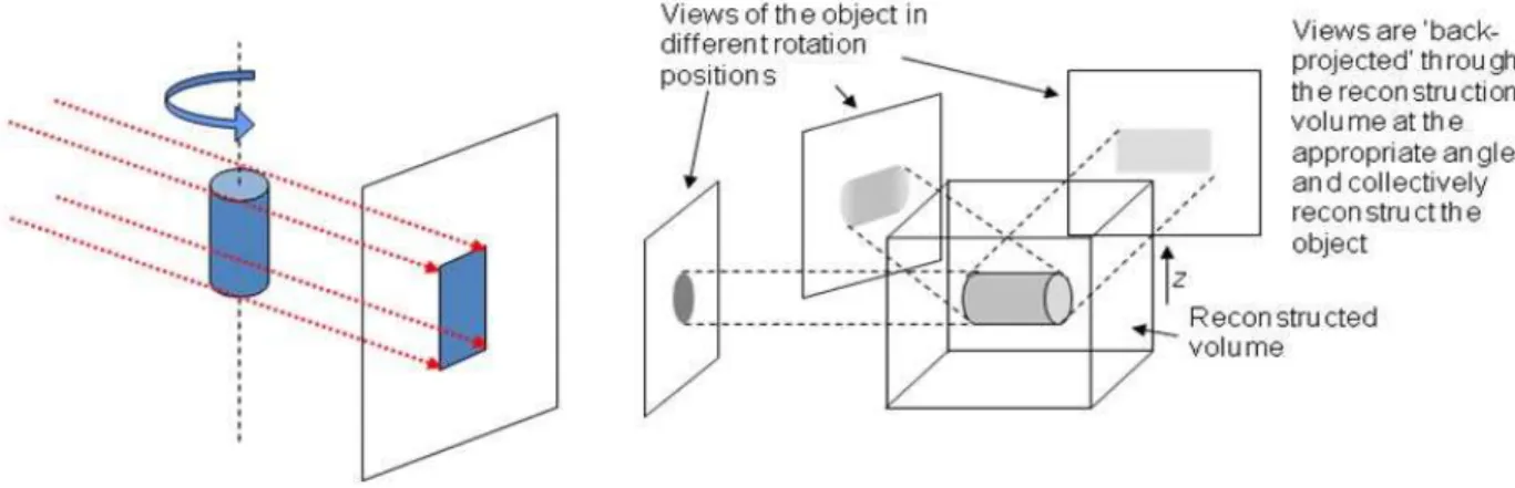
Figure 17 shows to the left a series of images due to X-ray transmission, the slices are acquired when the sample rotates around the vertical axis. On the right: these 2D views are mathematically back-projected through a 3D reconstruction volume (49).
Figure 17: Basic back-projected and reconstructed volume
The phase retrieval methods in general have a general pattern of measured intensity for the calculated Fourier transform ℱ[𝑔(𝐼)], after multiplying by a filter in the domain frequency 𝐻𝑝⋅ ℱ[𝑔(𝐼)], calculate the inverse Fourier transform ℱ−1{𝐻𝑝⋅ ℱ[𝑔(𝐼)]} to obtain the filter quantity and take the function 𝑓 and obtain the phase 𝜑(𝑟𝑇) with respect to the image plane in the transverse position (48).
𝝋(𝒓𝑻) = 𝒇(𝓕−𝟏{𝑯
𝒑⋅ 𝓕[𝒈(𝑰)]}) Eq. 14 𝐼: Intensity in the image plane in the transverse position 𝐼(𝑟𝑇)
31
𝑟𝑇 : Position on the detector, 𝑟𝑇 = (𝑥, 𝑦) 𝜑(𝑟𝑇) : phase retrieval function
ℱ: Fourier transform
𝐻𝑝: filter in the frequency domain 𝐻𝑝(𝑤) ℱ−1: Inverse Fourier transform
𝑓: function for obtaining the phase
There are various phase retrieval algorithms (50) (51) which produces images analogous to the pure absorption contrast images, also reducing noise significantly, producing a cleaner reconstruction.
Besides it enables us to obtain quantitative information on the samples from phase-contrast images, it works best in the near field or close to it (44).
The algorithm of phase reconstruction used for the beamlines SYRMEP/Elettra and ID-17/ESRF was Paganin algorithm (52) :
𝝋(𝒙, 𝒚) = 𝜹
𝟐𝜷𝐥𝐧 (𝑭
−𝟏{ 𝑭[𝑰(𝒙,𝒚)/𝑰𝟎(𝒙,𝒚)]
𝟏+[𝝀𝒛𝜹/(𝟒𝝅𝜷)](𝒖𝟐+𝒗𝟐)}) Eq. 15
With:
z: distance between object and detector
d: characteristic size of the smallest discernible features in the object
λ: X-ray wavelength
(x, y): coordinates in the image and/or object plane 𝐼0(𝑥, 𝑦): incident intensity just upstream of the object
I (x, y): intensity distribution
F: direct Fourier transform operator 𝐹−1: backward Fourier transform operator
32
𝜹: decrement from the unity of the x-ray refractive index of the object and are related to the complex-valued x-ray refractive index n, from Eq. 1. u and v: the complex conjugate coordinates of x and y respectively
Equation 15 is valid if:
- the object is a homogeneous material, - if monochromatic radiation is used
- The distance z between object and detector is a near-field condition.
The ratio δ/β is an input parameter for the phase-retrieval, not the explicit values for β and δ, or in cases where the exact chemical composition of the sample material is unknown.
The sample-to-detector distance can be large enough to enhance the phase-contrast and applied to a Paganin filter (53).
33
Chapter II
Hardware
34
2. Hardware System
Microtomography System
A single source and a detector made up the first scanner generation. It had limitations but can be extremely useful in µCT. This system has the advantages of relatively low set-up cost and excellent results for different types of measurements (54).
The commercially available components from a typical cone-beam micro-CT machine are an X-ray tube, a rotary stage, and a high-resolution detector (see Figure 18) (55).
Figure 18: Typical cone beam micro-CT machine
The X-ray flux is an important factor for microtomography operation: an optimal energy source is needed that allows a greater number of photons to uniformly penetrate the material, depending on factors such as signal noise and the diameter of a sample. A further important aspect is that the X-ray power should be maintained constant over the data acquisition time (56). The main difference of micro focus-CT systems in relation to Synchrotron Radiation µCT is linked to the X-ray source features. Figure 19(a) schematically shows that the synchrotron radiation produces monochromatic parallel beams whose divergence is 10-5 rad. Figure 19(b) indicates a micro-focus source with a polychromatic cone beam which diverges on 1 rad (57).
The smaller the spot size, the smaller the penumbral blurring, which will help produce a more accurate projected image. A larger spot size means that photons hitting a specific pixel can be traced back through different ray paths through the specimen (2).
35
Figure 19: Difference between microfocus-CT systems and synchrotron system
The collimator is a component which permits the X-ray beam geometry to be focused in a fan- or cone-beam projection. A typical detector in microtomography system is a CMOS or CCD detector coupled with a phosphor (scintillator) screen (9). The sCMOS (Scientific CMOS) technology is now able to deliver performances that hybrid CCD/CMOS technology cannot: a unique combination of sensitivity, speed, dynamic range, resolution, and field of view (58). The sample composition and size determine which X-ray spectrum should be used (energy range). Another important parameter is the pixel size of the detector, the spatial resolution is equal to the pixel size divided by the magnification (59). The magnification ratio of the projection data is determined by SDD/SOD where SDD and SOD are the detector and source-to-object distances, respectively (see Figure 20) (60).
36 Acquisition in Microtomography
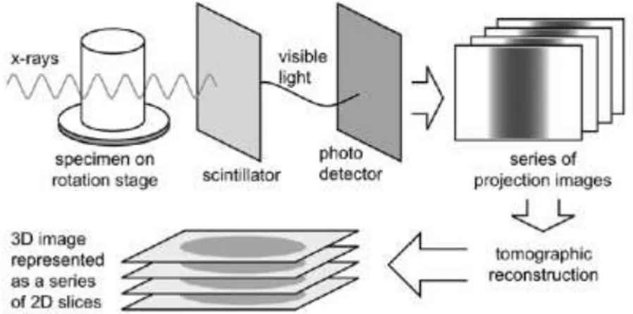
As already noted, a series of X-ray projected images is acquired and mathematically reconstructed to produce a 3D map of X-ray absorption in the volume. The 3D map is typically presented as a series of 2D slice images (see Figure 21) (2).
Figure 21: Schematic illustration of X-ray CT acquisition and reconstruction processes.
Acquisition of 2D radiographs require appropriate scintillation, to convert the X-rays to visible light, and detectors to produce a digital image. The application of 2D detectors allowed the acquisition matrix of data which represents 2D projection images, leading to faster scan times (2).
Syrmep Beamline - Elettra Sincrotrone Trieste
The beamline SYRMEP is part of the Elettra Sincrotrone located in Trieste, Italy. The 6.1 bending magnet source produces a laminar polychromatic beam that is shaped by using a vacuum slit system. A monochromator, based on a double-Si (111)-crystal, allows to obtain a monochromatic beam with an energy between 8 keV and 35 keV. An air slit system delimits the beam before entering the ionization chamber for the measurement of its intensity. At this point, the monochromatic incident beam enters the beamline SYRMEP
37
with a typical useful area of 210 mm x 5 mm at 20 keV. The sample stage is provided with 6 motors (M1-M6) for a fine positioning of the sample (see Figure 22) (61).
The measurement procedure involves, prior to the scanning, the alignment of the system (motors and slits) and the tuning of the optimal. The following step of the acquisition consists of fixing the number of rotational steps. Normally, before and after the sample scanning, acquisition of flat/dark field images is performed for the normalization in the reconstruction process (processing of the image). The first step of image post-processing is obtained by extracting the sinograms (61). The reconstruction of the of both absorption and contrast phase tomographic images is obtained by the STP (SYRMEP Tomo Project) (62).
The graph indicated simulation using a cubic sample with three white holes for scanning over the rotator plate until 1800 in the pre-processing image step shows the intensity profile in 1800, afterwards the reconstructed image from a sinogram is in the form of a 2D reconstructed image.
In Figure 22 we illustrate, enclosed by an orange dashed line, the part of our interest in the SYRMEP system, which comprises the programming of the apparatus control and data acquisition.
ID17 – Beamline - ESRF Grenoble
The ID17 is a biomedical beamline, part of ESRF - the European Synchrotron Radiation Facility, located in Grenoble, France, involving both diagnostic imaging and therapeutic irradiation for pre-clinical and potentially clinical application (See Tables 1-3) (63).
38
39 Table 2
Table 3
The X-ray beam is generated by an 11-period wiggler with a maximum magnetic field 1.592 T at a wiggler gap (Figure 23). The probed object is moved vertically through the beam while the CCD camera constantly acquires projection images (64).
Figure 23: ID 17- Schematic description of the imaging setup.
The ID17 wiggler is a neat way to increase the intensity of synchrotron radiation. It is a periodic arrangement of dipole magnets generating an alternating static magnetic field which deflects the electron beam sinusoidally (65). The filters are also placed as beam attenuators. They are located between the source and the sample to avoid overheating of the optical elements in the optic hutch (66).
STAR Facility
The STAR facility at the University of Calabria, in Rende (CS, Italy), is currently under commissioning. STAR source is the first user-facility, created for the
40
material science community based on the Thomson Backscattering (or inverse Compton) effect. The STAR source is formed by a S-band photo-injector producing 5 MeV electron bunches at 100Hz, a S-band LINAC accelerating the electrons up to 60 MeV feed by a dedicated Klystron; an integrated laser system constituted by two lasers (one feeding the photo-cathode of the photo-injector, one driven to the interaction point). X-rays are emitted for the Thomson Scattering mechanism when the accelerated and focussed electron bunches collide with the focussed laser beam. The X-rays collected in the backscattering geometry are polarized, monochromatic, tuneable with continuity between 40 and 140 keV, shaped in pulses of a of few picoseconds duration and with a flux of the order of 109 photons/s (67) (68) (See Figure 24).
Figure 24: STAR Facility
µTomo Laboratory at STAR
µTomo Laboratory is part of the STAR-Lab facility realized under the PON MaTeRiA project. It is located into the University of Calabria campus in Italy. The µ-Tomo Experimental Station consists of three precision optical tables Thorlabs mod. B6090B, equipped with a microfocus X-ray source, five motion cradles, and a flat panel detector. The sample handling system provides four degrees of freedom, while the fifth degree (phi), corresponding to one of the cradles needed for sample alignment, is placed under the detector to reduce the weight to be manipulated. This system allows to position with
41
the required sample precision up to 80 mm in diameter and 6 kg in weight. The particular arrangement of the actuators enables tomography to be performed both in full beam mode (where all the irradiated sample is always contained in the field of view of the detector during rotation) and in the half-beam one (where the maximum dimensions to be captured exceed the maximum transverse dimension of the detector, but no more than a factor 2). Some features of the system are shown in Table 4 with reference to Figure 25.
Specifications
PI-Micos Model LS-270 LS-180 WT-90 WT-90 PRS-110
Load Capacity (Kg) 150 100 8 8 10
Load Capacity (N) 1500 (Fz) 200 (Fy) 80 (Fz) 80 (Fz) 100 (Fz)
Travel range 205 mm 155 mm 90° (max) 90° (max) >360° Bi-direc. Repeatability (down to) 0.05 µm 0.05 µm 0.001 ° 0.001 ° 0.0002° Maximun speed (mm/s) 150 200 15 15 200
Type limit switch
Inductive (pnp) NC
mechanical
(pnp) NC npn* npn* npn*
Location on µ-Tomo
Station X-axis Y-axis Phi Tetha Omega
NC: Normal-closed * : internally by jumper
Table 4: Motors Characteristics
42
The µTomo station is provided with a user interface that allows its control through a personal computer. In particular, give the possibility of:
• Place the sample (4 degrees of freedom); • Orient the detector (1 degree of freedom); • Set the operating parameters of the detector; • Acquire images from the detector.
The Microfocus X-ray source is the Hamamatsu L12161-07 one whose main characteristics are:
Parameter Value Unit
X-ray tube voltage setting range 0 to 150 kV X-ray tube current setting range 0 to 500 μA X-ray tube voltage operational range 40 to 150 kV X-ray tube current operational range 10 to 500 μA Maximum output
- Small Focus Mode 10 W
- Middle Focus Mode 30 W
- Large Focus Mode 75 W
X-ray focal spot size (Nominal value)
- Small Focus Mode 7 (5 μm at 4 W) μm
- Middle Focus Mode 20 μm
- Large Focus Mode 50 μm
X-ray beam angle Approx. 43 degree
Focus to object distance (FOD) Approx. 17 mm Table 5: Microfocus characteristics
The used detector is a Flat panel sensor C7942SK-05 from Hamamatsu – Japan. Its main features are:
Parameter Value Unit
Energy range: 150 kVp Max.
High quality image: 5.4 Mpixels
Pixel size: 50 × 50 μm
Digital output (12-bits)
High-speed imaging: 2 frames/s (single binning)
9 frames/s (4 × 4 binning)
43
The whole system allows to control the X-rays test source managing; the sample-under-test (SUD) moving, using five high precision stepper motors; the image acquisition, by means of a at panel detector, subsequent made the 2D and 3D image reconstruction, thanks to an open-source reconstruction tool.
The micro-tomographic experimental station, named µTomo, was set up to exploit the hard X-rays produced by the STAR source. Both, the electronic hardware and mechanical design of the µTomo system was realized by Elettra Sincrotrone Trieste SCpA. Currently, the µTomo Laboratory is equipped with a micro-focus X-ray tube and a flat panel for µ-CT; these devices are remotely managed from a control room for the images acquisition.
All the electronic hardware components are commercially available and are, in general, provided with software drivers which are LabVIEW compatible (55).
The microtomography system is equipped with reliable components such as the stepper motors: low cost, can work in open loop, excellent holding torque and low speeds, low maintenance (brushless), very rugged in any environment, excellent for precise positioning control and no tuning required (69).
“Figure 26” shows the mechanical assembly of the µTomo STAR Experimental Station. There are five motors for each degree freedom in the experimental station:
• A goniometer WT-90, 2SM, MLS model corresponds to the Φ axis. • A goniometer WT-90, 2SM, MLS model corresponds to the θ axis. • There is a rotator PRS-110, 2SM, MLS model.
• A translator LS-270 model corresponds to the x-axis. • A translator LS-180 model corresponds to the y-axis.
The goniometer WT-90 designed for all tasks where conventional rotation stages cannot be used due to limited space conditions (70). The two goniometers are mounted orthogonally under the rotator with a common center of rotation.
The Linear Stage LS-270 was developed for positioning tasks with high loads, up to 150 kg andallows velocities up to 150 mm/s (71).
44
LS-180 Linear Stage for heavy loads had high travel accuracy and load capacity up to 100 kg andallows velocities up to 200 mm/s (72).
The detector, a C7942SK-05 flat panel sensor, is a digital image sensor newly developed as a key device for non-destructive inspection and for X-ray imaging applications requiring high image quality. Its principal characteristics are 150 KVp max., resolution of 5.4 Mpixels, the pixel size of 50 x 50 µm and high-performance GOS scintillator (73) (See Table 7).
Table 7: C7942SK-05 - Functional Specification
The detector moves manually over a rail in the z-axis. At full performance, it uses an external frame grabber board, in binning or trigger operation.
The microsource is a Hamamatsu model L12161-07 whose features are a minimum focal spot size of 5 µm at 4W, 75 W maximum output, 42° cone aperture and a control via the RS-232C interface (74) It can move manually along the y-axis and z-axis in the alignment process.
45
The equipment is schematically depicted in Figure 27. Two motors (WT-90 model) are attached to axis-1 and axis-3 connectors, respectively, while a third one (PRS-110 model) is attached to axis-2 one of the Corvus-Eco controller, which in turn is an interpreter of Venus-1 commands. The motors of the linear translation (model 270 and model LS-180) are attached to axis-1 and axis-2 connectors of the Hydra controller. The Corvus-Eco controller, the Hydra controller, and the X-ray Control Unit are connected over the serial interface to Moxa Nport. Finally, the Moxa Nport and CMOS flat panel sensor are connected with Cat 5e UTP to the server and room control, respectively.
46
An isometric view of the µTomo Experimental Station is reported in Figure 28. Here, we show the sample placement into the FOV and the ROI.
Figure 28: Alignment of experimental station
Regarding the EPICS connection, the upgraded hardware consists of adding a client and EPICS server to the network for µ-CT experiments. The control based on LabView over EPICS platform was developed at the µ-Tomo Laboratory of the STAR facility, sited at the University of Calabria, Italy. The versatility of system permits operated with microfocus (µTomo Laboratory) or TBS source over EPICS platform and permit exploit all the characteristics of light (See Figure 29).
Hardware Beamline Syrmep for acquisition
The µTomo beamline is like the SYRMEP one, illustrated in Figure 30, as concern the diagram of connection. The remote control from client to server is given by a UTP line while the server is connected to the sCMOS detector and to the rotator by means of a Moxa and a Mercury Controller.
47
Figure 29: EPICS - Connection Diagram
48
Chapter III
49
3. Software Development
The µTomo software was development using LabVIEW to control the hardware by means of a graphical user interface (GUI). LabVIEW is a graphical programming language. It has a powerful function library and an easy-to-use multithreaded programming and graphic user interface (GUI) design. The availability of drivers, debugging, and other features make it an ideal software for instrument-oriented programming (75).
The developed software is flexible allowing easy changes or additions of the hardware. The RS232 serial interface is the communication standard for most of the used laboratory equipment (Microfocus X-ray source and motors).
The Main Program
The main program was created using the 2015 version of LabVIEW. An installer is also created to be executed in computers without LabVIEW already installed or with older version of the same program. The software can be used on both 32 bits or 64 bits Windows environment.
Figure 31 shows the front panel of the Main Program while Figure 32 depicts a synthesized code of the Block Diagram which consisted in three subroutines, two for the motors and one for the acquisition sequence respectively. The front panel has a menu divided into four parts: ‘Phi/Theta’, ‘X-Y-Rotator’, ‘Acquisition’ and ‘File Parameters’ for the complete control of the µTomo apparatus.
50
Figure 31: Front Panel
Figure 32: Block Diagram 3.1.1. Control Motors
The motor control programming was carried out taking as a reference the software TestProgram.vi of the Mechanische Instrument Optische System (Micos) (76).
51
3.2.1.1. Creation of independent menu for 2 axes (Phi/Theta)
Figures 33-35 show the code for Phi/Theta control for axis-1 and axis-3 respectively. This menu permits the Corvus controller to work for stepper motors:
Phi: Axis 1: WT-90, 2SM, MLS Theta: Axis 3: WT-90, 2SM, MLS
The menu allows to verify the communication status, eventual errors, the performed movements and to set the velocity and acceleration.
Furthermore, the following operation were implemented:
• Set the absolute movement for the two axes using an independent absolute step width for each axis such as shown in the diagrams in Figures 33 and 34:
Figure 33: Absolute movement - Axis 1
52
• Set relative movement only for two axes, using independent relative step width for each axis, (see Figure 35).
Figure 35: Relative movement
• Control the state of stop or end for the motors.
• Permit visualization of the position in real time for the two axes. Update the position of each axis every 50 ms
3.2.1.2. Creation of menu for rotation and X and Y movements
The menu depicted in Figure 36 is relative to the Corvus controller (control of the stepper motor relative to the axis rotator: PRS-110, 2SM, MLS) and of the Hydra controller (control of the stepper motor relative to the Y-axis - LS-270 - and X-axis - LS-180).
The front panel divided into two parts, the upper part refers to X-axis and Y-axis while the lower part is relative to the rotator. The programming is based on the Demo.exe program (78) (79) and permits setting the absolute and relative movements for the X-axis and Y-axis in the microtomography system by means of Ethernet and/or RS-232 communication. The characteristics of this menu are:
53
▪ Position: present position, returned from the controller for each axis. ▪ Relative movement: negative or positive direction.
▪ Absolute movement: the parameter is the target position starting at the present position.
▪ Stop: Stops motion of the axis ▪ Initializing of motors for each axis. ▪ Reset to zero the value of the position
▪ Initial Calibration: for alignment of sample using ncal and nrm buttons.
Figure 36: Control rotation, x and y movements
Figure 37 shows the ‘view-file’ tab, permitting opening and uploading the configuration file with txt extension. The actual configuration is also reported: the status bits permit the principal activities of the hydra controller to be displayed. If the motor power is disabled,
54
it is possible to use the "Init" button for enabling the power; this procedure is necessary to initialize the controller. A series of Boolean variables are displayed to show the status of the apparatus. As an example, in the next figure, the label "Axis is moving" is ON because a relative or absolute movement is under way.
Figure 37: Hydra – View file
An error handling procedure is also coded: while the ‘machine errors’ virtual led is off then bit 4 is 0FF, but the condition for the error may not be removed (emergency stop is active). In all these cases, the bit 8 is active and shows an enlighten virtual led. If the emergency condition is removed, then it is necessary to press the button ‘Init’ to activate the power stage of the controller and no reset must be sent to the hydra controller (79). Among other modifications made to the program we have the setup the absolute
55
movement for one axis, using an independent absolute step width for each axis. (see Figure 38):
Figure 38: Absolute movement for rotator 3.1.2. TCP/IP Acquisition
Figure 39 indicates the front panel of TCP/IP acquisition. Its menu allows: • Inserting of the number of images to be collected (up to 9999)
• An image counter which shows the current number of the acquired images. • Giving a prefix for each image filename; dark, flat and projection are set
automatically
• Stop the acquisition by using the button "Exit All Programs". • Set and read the exposure time..
Figure 40 shows a typical parameter file that can be updated by the user to insert the acquisition parameters prior to scanning. The program saves the parameter file automatically in the same folder of the acquired images.
Figure 41 indicates the block diagram for the acquisition procedure. As a preliminary step, the input signal calibration is needed, allowing the control of the acquisition parameters of each image in accord with the movement of the rotator.
56
Figure 39: Front Panel - TCP/IP Acquisition
57
Figure 41: Block diagram – Acquisition
3.1.3. Subprograms Link
The remote acquisition procedure consists on the setting of the motors positions according to the size of the sample for a suitable acquisition. Successively the acquisition module is linked to the rotator control module. The signal "Image Ready" indicates when an image is acquired (see Figure 42).
58 Upgraded to EPICS I/O Server
EPICS is a set of Open Source software tools, libraries and applications developed collaboratively and used worldwide to create distributed soft real-time control systems for scientific instruments (80).
EPICS was choosen as the software environment for the control of the STAR infrastructure and, thus, there is a need to let the whole µTomo acquisition process be controlle by a proper linkage between this software and Labview.
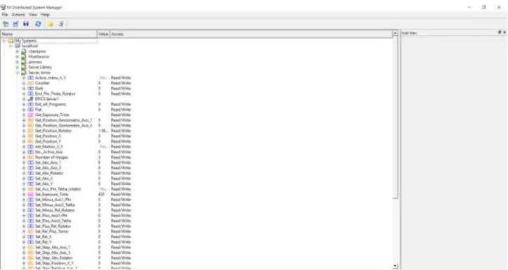
The linking of the Epics Server with the LabVIEW environment consisted in creating a LabVIEW Project containing both the necessary VIs (virtual instruments) and PVs (Process Variables) (see Figure 45). LabVIEW module allows the user to read, initialize or monitor the state of the networks variables (see Figure 46) by using DSC (Data-logging and Supervisory Control). The developed Epics client GUI, by controlling these variables, makes the µTomo images acquisition possible. The Epics server manages the channel access to network variables and allows it to be read by an Epics client. A Distributed System Manager allows monitoring the Epics Process Variables.
Figures 43 and 44 show the front panel and block diagram of the Epics Server.
59
Figure 44: Part of block diagram – Epics Server
60
Figure 46: Monitoring Epics Process Variables with Distributed System Manager
Alternative Software for image acquisition – SYRMEP beamline @ Elettra
During a period spent at Elettra Sincrotrone (Trieste), a similar software was developed for image acquisition by remote control on TCP-IP at the SYRMEP beamline. Figure 47 shows the code on LabVIEW for the “detector control” and the “rotator control”.
The sCMOS detector connected to the server is controlled on the TCP/IP of the client. As a starting point, it is necessary to configure the communication parameters, by starting the server and verifying the communication.
For the rotator, it is necessary to configure the serial communication parameters of the C-863 Mercury Controller connected to the rotator. Figure 47 indicates the blocks of acquisition: range of images for select the number of images for acquire, generator of names for each image and communication of commands for transmission and reception. The rotator is verified its rotating, when the control the response to the specific command
61
'ONT?’. Also, in this case, the initial settings for image acquisition should provide the number of images before acquisition.
Figure 47: Alternative Software for acquisition image
Development of Graphic User Interface (GUI) in Python Language – ID17 beamline @ ESRF
A Graphic User Interface (GUI) was developed in Python Language for ID17 beamline in ESRF (Grenoble – France). It was designed for online image reconstruction during experiments. Autonomous handling of reconstruction software and the specific routines were developed for the specific users.
The main goal of the GUI is to provide a user-friendly multi-technique platform that can be used to handle the data obtained with different phase-contrast techniques like Propagation-based imaging (PBI).
62
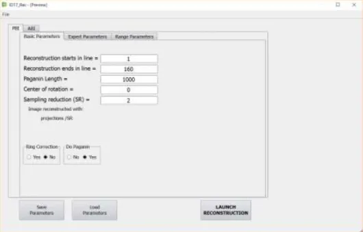
The code was structured into different classes and methods. PyQt, a Python graphic tool, brings together the Qt C++ cross-platform application framework and the cross-platform interpreted by the Python language (82). The PyQt library is used for the GUI. PyQt is a set of Python v2 and v3 multiplatform bindings. Figures 48 and 49 illustrated the templates:
Figure 48:Template of Basic Parameters
63
The template program is linked to the functions grouped into classes in the python code, according to the python code made by Alberto Mittone, scientist of ID17 beamline staff. The template generates a text file, according to the instructions manual of ID17 (83) For details, see the Annex 1.
Figure 50: Template of Range Parameters
The main parameter that are controlled by the ID17 GUI are:
COR range (Center of rotation)
This parameter allows linking to the script to reconstruct a single slice of the volume concerned using different centres of rotation in the range. The CT files are saved in the COR folder. The folder is created automatically (see Figure 50).
Delta-Beta range
This parameter allows linking to the script to reconstruct a single slice of the volume concerned using a different specific parameter (Paganin number) in the range. The CT files are saved in the PAG folder. The folder is created automatically (see Figure 50).
64 Software operation mode
The GUI allows the following operations:
• “Save Parameters” Boolean controls the writing of the user and basic parameters used for reconstruction in a text file.
• “Load Parameters” Boolean controls the updating of the user and basic parameters reconstruction from a text file.
• The possibility of performing reconstructions automatically using a range of parameters (i.e. different centres of rotation and different values of delta/beta values using a single distance for the non-iterative phase retrieval algorithm described by David Paganin) (84). Phase retrieval enables us to obtain quantitative
65 Flowchart
66