MOLECULAR MODELLING STUDIES OF THE NF-κB BIOLOGICAL SYSTEM AS RELEVANT DRUG TARGET

(1)

Università degli Studi di Ferrara

DOTTORATO DI RICERCA IN

BIOCHIMICA, BIOLOGIA MOLECOLARE E BIOTECNOLOGIE

CICLO XXI

COORDINATORE Prof. Bernardi Francesco

MOLECULAR MODELLING STUDIES OF THE NF-κB BIOLOGICAL SYSTEM AS RELEVANT DRUG TARGET

Settore Scientifico Disciplinare BIO/10

Dottorando Tutore

Dott. Piccagli Laura Prof. Gambari Roberto

(2)

CHAPTER 1. General introduction

1.1 Molecular modelling in drug discovery

An increasing number of drug discovery projects have applied bioinformatics disciplines, one of the fastest growing fields in science.1_{Major application of bioinformatics concern}

sequence alignment, genome assembly, gene expression prediction, protein structure prediction, protein-protein and protein-ligand docking, and molecular dynamics simulations.2 Moreover, the number of such projects is expected to continue to rise due to the Human Genome Project and high-throughput X-ray crystallography efforts.

Molecular modelling is a general name that concerns computational techniques and theoretical methods to model or simulate the behaviour of molecules.3 Nowadays these techniques are applied in the fields of computational biology, computational chemistry and materials science for studying molecular systems ranging from small chemical systems to large biological molecules and material assemblies. In particular, the synergy between biological experimental and computational studies has greatly benefited both fields, providing invaluable information in many different areas of the life sciences.4

The historical process of developing concepts leading to molecular modelling started with the quantum chemical description of molecules. This approach yields excellent results on the ab- initio level, but the size of the molecular system which can be handled is still rather limited. Therefore, the introduction of molecular modelling as a routine research tool is due to the appearance of new technologies in computer graphics together with the development of molecular mechanism about 30 years ago. Moreover, the development of more accurate and reliable algorithms, the employ of more thoughtful protocols to apply them, and greatly increased computational power nowadays permits studies to be performed with the necessary reliability and accuracy. Thus, theoretical calculations, three-dimensional visualisation and manipulation of molecular systems can be used to gain new ideas and reliable working

(6)

The process of drug discovery involves the identification of candidates, synthesis, characterisation, screening, and assays for therapeutic efficacy. Once a compound has shown its value in these tests, it will begin the process of drug development prior to clinical trials. Despite advances in technology and understanding of biological systems, drug discovery is still a long process with low rate of new therapeutic discovery.5,6

A fundamental postulate in medicinal chemistry is that most drugs produce their effect in the human body as a consequence of the molecular recognition between a small ligand (the drug itself) and a biological relevant macromolecule (the target) such as an enzyme, DNA, glycoprotein or receptor. Thus, a key activity of early drug discovery involves the identification of small molecule modulators (lead compounds) of a target function.

The virtual screening (VS) is a computational approach to screen large of small compounds virtual libraries for the discovery of interesting biological active lead candidates against biological target, especially proteins.7,8 The expression ‘virtual screening’ , coined in the late 1990s, was adopted by the scientific community in an effort to show that this in silico method is a serious alternative (or complementary) to the well-established HTS techniques.

In some studies reported in literature, the virtual screen had 'hit rates' (number of molecules that bind at a particular concentration divided by the number of compounds experimentally tested) that were 100-fold to 1,000-fold higher than those reached by empirical screen.9,10 When used prior to experimental screening, VS can be considered as a powerful computational filter for reducing the size of a natural or chemical library that will be further experimentally tested. Of course, experimental drawbacks, such as organic molecules availability, limited solubility, aggregate formation or any sort of physical properties of substance material that could possibly interfere with the applied assay conditions do not need to be considered in the first phase of a virtual screening application.

This mean that VS can permit a more flexible evaluation of the chemical space of molecules and the creation of focused libraries that could comprise not necessary existing different chemical structures. Moreover, VS represents a quite good alternative for growing demand of faster and relatively cheap screening of small molecule driven by genomics and combinatorial chemistry. Structured based virtual screening method is based on the application of molecular docking technique which is designed to find the correct orientation and conformation (pose) of a ligand into the binding site of a target.

(7)

The knowledge of a well defined three-dimensional (3D) structure of the biological target under study must be available as starting point for the application of this strategy for finding new leads. Docking studies have now been used with different success for decades. Once the ligand has been docked, it should be scored according to the tightness of target-ligand interactions. The capability to correctly predict ligand-protein interactions is fundamental to any accurate docking algorithm and the necessary starting point for any reliable virtual screening protocol. In fact, information about the fit of molecules into the target is then used to rank the compounds with the aim of selecting and experimentally test a small subset for biological activity. The use of multiple receptor conformations in ligand docking seems probably the best choice to date.

Molecular dynamic (MD) is a computational method for obtaining all information about the dynamic properties of a protein, among them possible conformations states. Thus, in order to take in consideration the receptor flexibility in docking application, molecular MD technique could be of help. MD is a simulation of the time-dependent behaviour of a molecular system.11 The addition of the time as forth dimension to structural biology allows that the positions in space and time of all atom in a protein can be described in detail. Although static structures are known for many proteins, the variety of functions of complex macromolecules is governed ultimately by their dynamic character.

The NF-κB consists of a group of eukaryotic inducible proteins that have evoked widespread interest until now.12 In spite of the well-defined solved NF-κB 3D structures, to the best of our knowledge, nowadays VS applications against this interesting target for the discovery of new NF-κB/DNA inhibitors have not been published yet. The investigations described in this thesis bear upon the application in silico methodologies focusing on structured-based virtual screening against NF-κB transcription factors family.

1.2 Aim and outlines of this thesis

The project described in this thesis is aimed to the identification of low molecular weight compounds interacting with NF-κB and able to inhibit DNA/NF-κB complex formation and biological dependent functions. The short introduction described in the previous section clearly illustrate that structured-based VS has played an important role in lead compounds

(8)

discovery. In Chapter 2 a literary survey and clearly description is given on computational methods to be applied and on the targets under study. Chapter 3 deals with the implementation of a docking protocol suitable for NF-κB p50 monomer and homodimer. As a first step towards the development of an effective procedure, a data set of 27 bioactive natural compounds and two known NF-κB p50 binders were employed. We found that the adopted sampling method and the scoring function were successful in predict the ranking of active and inactive compounds into DNA binding site of the ensemble protein. The application of docking runs for the VS of a purpose-made prepared large chemical library is presented in chapter 4. A successful identification of a micromolar active compound structurally correlated to a substituted coumarin is described together with its binding modes. In chapter 5 a focus library of 1700 furocoumarin derivatives was prepared and in silico screened against NF-κB p50. Further in depth investigations of resulting five bioactive interesting hits against NF-κB p50 homodimer and p50-p65 heterodimer are reported revealing substantial differences. Binding studies on the best poses in the homodimer showed the involvement of an essential residue for p50 in vivo activity in ligand/homodimer interaction. Finally, in chapter 6 molecular dynamic simulations on NF-κB p50-p65 in three different systems (free form, in complex with DNA and bounded to IκBα) are presented. The dynamic properties and the most relevant protein conformations in different systems have been analysed in order to enlarge and optimise the VS strategy against the most common NF-κB heterodimer p50-p65.

(9)

References

1. Setubal CJ, Verjovski-Almeidaet S: Advances in Bioinformatics and Computational Biology. Brazilian Symposium on Bioinformatics, BSB held in Sao Leopoldo, Brazil, 2005.

2. Marcus F: Bioinformatics and Systems Biology: Collaborative Research and Resources . Springer, 2008. 3. Leach. AR: Molecular Modelling: Principles and Applications . Pearson Education, 2001.

4. Ciobanu J, Rozenberg G: Modelling in Molecular Biology . Springer-Verlag, 2004.

5. Kong D, Li X, Zhang H: Where is the hope for drug discovery? Let history tell the future. Drug Discov Today in press.

6. S kraljevic, P J Stambrook, K and Pavelic: Accel. Drug discovery. EMBO 2004, 5, 837.

7. Chin D, Chuaqui C, Singh J: Integration of Virtual Screening into the Drug Discovery Process. Mini-Reviews in Med Chem 2004, 4, 1053.

8. Shoichet BK, McGovern SL, Wei B, Irwin JJ: Lead discovery using molecular docking: Curr Opinion in Chem Biol 2002, 6, 439.

9. Doman TN, McGovern SL, Witherbee BJ, Kasten TP, Kurumbail R, Stallings WC, Connolly DT, Shoichet BK: Molecular docking and high-throughput screening for novel inhibitors of protein tyrosine phosphatase-1B. J. Med Chem 2002; 45, 2213.

10. Paiva AM, Vanderwall DE, Blanchard JS, Kozarich JW, Williamson JM, Kelly TM. Inhibitors of dihydrodipicolinate reductase, a key enzyme of the diaminopimelate pathway of Mycobacterium tuberculosis. Biochim Biophys Acta 2001, 1545, 67.

11. Henzler-Wildman K, Kern D: Dynamic personalities of proteins. Nature 2007, 450, 964.

(10)

(11)

CHAPTER 2. Literature survey

2.1 Computational methods

2.1.1 Molecular docking

Docking simulations represent a widely employed computational tool in drug discovery field, which attempts to predict a manifold of structures of intermolecular complex between at least two objects. The first docking attempts were done manually using interactive computer modelling. The ligand is put in the binding site and minimised to avoid bad steric clashes. This approach can be effective if we have a good idea of the expected binding mode. However, X-ray structures have revealed that even very similar inhibitors can adopt different binding modes.

Usually, but not necessarily, docking programs search along the conformational degrees of freedom of a small molecule (the ligand) while the protein is treated as a rigid body.

The results of such a search are configurations, namely conformations associated to a particular spatial orientation of the ligand at the binding site, which are usually referred to as solution poses.

A standard docking protocol consists of a step-wise process. First, a proper search algorithm predicts the various configurations of the ligand within the target binding site. In the second step, each docked pose is evaluated and ranked assessing the intermolecular interaction tightness throughout an estimation of the binding free-energy. Ideally, the correlation between the most favourable free-energy values and the best predicted poses should be very straight. The ability of a standard docking protocol to achieve its ultimate goal providing a reliable binding mode prediction, strongly depends on the accuracy of the scoring function used.1,2

(12)

2.1.1.1 Algorithms for ligand conformational sampling

The treatment of ligand flexibility can be summarized into three basic categories: systematic, stochastic and genetic algorithms.3

Systematic methods attempts to cover all the conformational degrees of freedom exploring each of them in a combinatorial way. Such methods provide an exhaustive search only in the limit of very rigid or simple molecules; otherwise a combinatorial explosion of the search dimensionality occurs, yielding the approach unfeasible. In order to avoid this, termination criteria are usually implemented which focus the sampling along regions of the conformational space that are more likely to lead an effective solution (“search and grow algorithms”).

Conversely, stochastic approaches operate randomly selected changes along both the conformational internal and global (orientational/translational) degrees of freedom of the ligand, attempting to reach the global minimum for the molecule inside the binding site (Monte Carlo implementations). Within the Metropolis acceptance criterion, if the i-th solution of the conformational search bears an energy lower than the previous one (downhill move), it is always accepted. On the contrary, if the energy increases, a Boltzmann weighted probability function is then computed:

⎟⎟ ⎠ ⎞ ⎜⎜ ⎝ ⎛ − _∆ ∆ − ₌ = ∆E e E e kBT E 1 ) ( ) ( β ρ (2.01)

where ∆E is the energy difference between the i-th and the (i-1)-th configurations. To accept an uphill move with the probability ρ(∆E) a random number is uniformly generated in the range {0, 1}. If the random number is less than ρ(∆E) then the uphill move is accepted, otherwise it is rejected. Here, an higher temperature can be usually applied to explore a wider potential energy surface. The search is then interrupted when the desired number of configurations is obtained.

Genetic algorithms also implement a different amount of randomness; hence they should be formally classified between the stochastic ones. Nevertheless, compared with the properly called stochastic methods, they differ in the sense that they are based upon the principles of biological evolution and population dynamics, rather than on the laws of physics. Model

(13)

parameters representing the degrees of freedom are encoded in data strings called “chromosomes”. Such chromosomes are evaluated by a proper fitness function, and individuals whose chromosomes bear the largest fitness values have a better chance to reproduce and indeed to transmit their genetic inheritance to the next generation. Chromosomes are randomly varied by means of genetic-like operators, usually mutations and crossover, in order to increase density and prevent premature convergence. When applied to the docking problem, the genetic algorithm solution is a population of putative ligand conformations. For instance, in the software AutoDock 3.0.5, genetic algorithm represents an hybrid search technique that implements an adaptive genetic algorithm with a local search feature. The local searcher performs an energy minimization after the global sampling, hence the local changes occurred due to minimization are mapped back into the chromosomes. Since inheritance of acquired traits clearly contravenes the Mendelian genetic laws, in this sense the genetic algorithm is named “Lamarckian” after the discredited evolutionary theory of Lamarck.

Similarly, another popular docking suite such as GOLD, employs a genetic algorithm whose most remarkable feature is the migration genetic operator. At the beginning, several subpopulations of chromosomes, called islands, are created instead of a large unique population. In order to preserve diversity, individuals are allowed to move among islands through the migration operator. Finally, only a fixed number of individuals can share the same place within an island. If there are more than a specified number of individuals in the same place, then the new individuals replaces the worst scoring member in the place, and not the worst individual in the overall population.

2.1.1.2 Scoring functions for docking poses evaluation

Once a pose has been generated for a docked compound in its binding site, it needs to be scored to rank the quality of the pose with respect to other poses for the compound itself, and with respect to other molecules in the library. In order to evaluate the interaction energy between the target and each docked ligand, different scoring functions has been developed. There are several requirements a useful scoring function should satisfy. Firstly, in a virtual screening simulation, the scoring function should be able to discriminate between correct and incorrect binding modes of known ligands with reasonable accuracy and speed. Secondly,

(14)

The quantitative modeling of receptor-ligand interactions can be achieved by determining the equilibrium binding constant Keq, which is in turn directly related to the Gibbs free- energy:

S T H K RT G=− _eq =∆ − ∆ ∆ ln (2.02)

Therefore, the ideal scoring function should be able to calculate accurate binding free energies.

The difficulties relying on the estimation of the free-energy by means of computational techniques is extensively covered in literature, hence just an overview focused on the docking field will be given here.

Docking simulations are at now usually performed in vacuo, although in principle implicit solvation models could be used as well. Nevertheless, in spite of their theoretical derivation, scoring functions are usually able to provide a proper assessment of the enthalpic contribution for the free-energy (a force field-like potential energy function), whereas the entropic contribution remains hard to estimate. The main entropic contributions to the stability of the receptor-ligand complex are provided by desolvation effects, and by the internal conformational degrees of freedom of the docked small molecule. Within the docking field, the need for a fast scoring method led to a number of different functions which bring various assumptions and approximations in the evaluation of modelled complexes. Widely employed approximations are:

scoring functions assume that the free-energy of binding can be approximated using a single structure, which is a reasonable assumption since the lower is the energy of the configuration, the larger is its contribution to the partition function; the bound state for the complex is the only explicitly considered, whereas unbound components are implicitly accounted for; the free-energy is approximated by a linear combination of several terms, while several forces involved in the complex formation are non additive.

Empirical scoring functions provide an estimation of the binding free-energy by summing up interaction terms derived from structural parameters. The development of scoring functions is based on the idea that binding energies can be approximated by means of a sum of not correlated terms, which are derived by regression analysis from experimentally determined structures whose binding mode are known. Such kind of scoring functions are simple and

(15)

intuitive, but their main drawback is that it is not clear whether they are able to predict the binding affinities for ligands whose structure is not covered among the training set.

2.1.2 Classical Molecular Dynamics simulations

The molecular structures are usually represented as static objects, but are actually dynamic entities. Dynamics simulations are useful in studies of the time evolution of a variety of systems at non-zero temperatures, including biological molecules in a variety of states, for example, crystals and aqueous solutions. The major applications of molecular dynamics include performing conformational searches, generating statistical ensembles and studying the motions of molecules. Thus many relevant macromolecular features such as phase space accessible, energetic, thermodynamic, structural, and dynamic properties can be studied. One of the most important use is to investigate the range of possible configurations that molecule may assume into phase space to numerically simulate its dynamics behaviour.4,5 In the classical dynamic simulation this can be realized by calculating a trajectory, that is a number of time-dipendent configurations through the integration of the Newton equations of motion and using empirical force fields.

In this scheme, the fundamental equation relies on the Newton’s second law:

i

f (t)=m_ia_i(t) (2.03)

wheref_i, m_i and a_i stand for the force, the mass and the acceleration of atom i respectively. The force at time t on atom i can be directly calculated from the derivative of potential energy

Vin respect to the coordinates r_i.

∂V

∂r_i = m

∂2_r i

∂t_i2 (2.04)

where the potential V is accounted for by means of the potential energy function provided by the force field.

(16)

For conservative systems (invariant potential function in time), the force acting on the ith particle is a function of the coordinates only. Since the potential energy function (which is independent of velocities and time) required for the force calculation is provided by the force field, initial velocities are solely required in order to evolve the system (as starting coordinates are obviously known).

Basically, starting velocities of all particles involved are initialized by random selecting from a Maxwell-Boltzmann distribution at the temperature of interest:

t i, f

( )

⎟ ⎟ ⎠ ⎞ ⎜ ⎜ ⎝ ⎛ − ⎟⎟ ⎠ ⎞ ⎜⎜ ⎝ ⎛ = = k T v m B i ix B ix i e T k m v 2 2 2π (2.05)

where k is Boltzmann’s constant.

Since it represents a Gaussian distribution, it can be easily obtained from a random number generator. Therefore, dynamics runs cannot be repeated exactly, except for forcefield engines that allow setting the random number seed to the value that was used in a previous run.

As a consequence of a continuous potential, the motion of all particles is tightly correlated, giving rise to a many-body problem which can not be analytically solved. To overcome this, equations of motions are integrated using a finite difference method, where integration is performed on discrete time intervals δt. By doing so, forces are constant during each time step, and consequently collisions are elastics.

Thus for each integration step, the forces at time t are calculated by differentiating the potential energy function:

= t i, f -

( )

t i t i V , , r r ∂ ∂ (2.06)

The force on an atom may include contributions from the various terms in the force field, and represents the most time consuming part for a molecular dynamics code. The equations of motions are then integrated by means of a suitable algorithm. It should be fast, ideally requiring only one energy evaluation per timestep, a little computer memory and permit the use of a relatively long timestep. There are different algorithms to use in MD, each of them

(17)

assumes that the positions and dynamic properties (velocities, accelerations, and so on) can be approximated by a Taylor series expansion. The Verlet algorithm6 represents a third-order truncation, and uses positions and accelerations (previously computed) at time t, and the positions from the previous step. The variants leap-frog Verlet algorithm are perhaps the most widely used methods in molecular dynamics. Starting with r(t), v(t− ∆t /2), and a(t) that represents position, velocity and acceleration at t, t− ∆t /2 and t respectively, it calculates:

) ( ) 2 1 ( ) 2 1 (t t v t t ta t v + ∆ = − ∆ +∆ (2.07) ) 2 1 ( ) ( ) (t+∆t =r t +∆tv t+ ∆t r (2.08) m t t t t ) ( ) ( +∆ =f +∆ a (2.09)

where f(t+ ∆t) is evaluated from−dV dr a r(t+ ∆t)

It should be point out that with this algorithm the calculated positions and the velocities are confused of an half timestep.

The choice of the size of the time-step is key parameter in MD primarily determined by a compromise between accuracy and speed of the calculation. Unfortunately by using a large time step to increase the speed of the calculation would lead to instability and inaccuracy of integration procedure. In most organic models, the highest vibrational frequency is that of C-H bond stretching, whose period is on the order of 10−14 s (10 fs). The integration timestep should therefore be about 0.5-1 fs. As a safe rule of thumb, the time-step should be approximately one tenth the time of the shortest period of motion. When using a constraint algorithm (such as SHAKE)7,8 a longer timestep is possible.

Summarizing, the global molecular dynamic algorithm start with the input initial conditions: (i) the potential interaction V , as a function of atom positions, (ii) the positions r of all atoms in the system, and (iii) the velocities v of all atoms in the system. Starting by this point, the

(18)

computed by calculating the force between non bonded atom pairs plus the forces due to bonded interactions and plus restraining and/or external forces. The potential and kinetic energies and the pressure tensor are computed. Subsequently, the movement of the atoms is simulated by numerically solving Newton’s equations of motion (see eq. 2.03). Finally, positions, velocities, energies, temperature, pressure, etc are stored, as required, in the output files.9,10

The important output of the MD run is the trajectory file which contains particle coordinates and, optionally, velocities at regular intervals. Since the trajectory files are lengthy, one should not save every step. To retain all information it suffice to write a frame every 15 steps, since at least 30 steps are made per period of the highest frequency in the system, and Shannon’s sampling theorem states that two samples per period of the highest frequency in a band-limited signal contain all available information. But that still gives very long files. So, if the highest frequencies are not of interest, 10 or 20 samples per ps may be acceptable. The user should be aware of the distortion of high-frequency motions by the stroboscopic eﬀect, called aliasing: higher frequencies are mirrored with respect to the sampling frequency and appear as lower frequencies.11

2.1.2.1 Essential dynamics

Analysis of extended molecular dynamics simulations of proteins in vacuum and in aqueous solution reveals that it is possible to separate the configurational space into two subspaces: (a) an “essential” subspace containing only a few degrees of freedom in which anharmonic motion occurs that comprises most of the positional fluctuations; and (b) the remaining space in which the motion has a narrow Gaussian distribution and which can be considered as “physically constrained”. If overall translation and rotation are eliminated, the two spaces can be constructed by a simple linear transformation in Cartesian coordinate space, which remains valid over several hundred picoseconds. The transformation follows from the covariance matrix of the positional deviations. The diagonalization of the covariance matrix of the coordinate fluctuations produces a set of eigenvalues associated to eigenvectors. In mathematics, given a linear transformation, an eigenvector of that linear transformation is a nonzero vector which, when that transformation is applied to it, changes in length, but not in direction. For each eigenvector of a linear transformation, there is a corresponding scalar

(19)

value called eigenvalue for that vector, which determines the amount the eigenvector is scaled under the linear transformation. Applied to the dynamic simulation analysis context, the eigenvectors represent the direction of motions and the eigenvalues the amount of the motions.

The essential degrees of freedom seem to describe motions which are relevant for the function of the protein, while the physically constrained subspace merely describes irrelevant local fluctuations. The near-constraint behavior of the latter subspace allows the separation of equations of motion and promises the possibility of investigating independently the essential space and performing dynamic simulations only in this reduced space.12

2.2 Structured-based Virtual Screening strategies

Structured-based VS (SBVS) covers a variety of sequential computational phases including the application of the docking method as described above. The Figure 1 reports the classical workflow of a SBVS approach, including further experimental studies.13 Essentially, molecules from a prepared virtual database are docked into the protein and a suitable scoring function is used to evaluate the binding affinity. Subsequently, the virtual hits are tested in biological assay for activity. Finally compounds showing biological activity (lead compounds) are further modified using computational methods, medicinal chemistry, structure–activity relationship and structural studies to get second generation compounds The enrichment factor (EF) for a library built with the n top compounds of the ranked library can be defined as:14

( )

total total n n N Hits N Hits n EF = _(2.10)

and expresses the relative change in the probability of finding a ligand in the focused library when compared to a random pick from the complete library.

The successful application of SBVS depends on a wide range of factors based on the information accessibility and computational techniques adopted on the case-study. Thus the EF can define in manifold modalities. In common with HTS, Brian K. Shoichet15 point out

(20)

that we can define success in VS as “finding some interesting new ligands”, and not as “correctly ranking all the molecules in a library” or “find all the possible ligands in a library”. In this chapter we describe some focusing considerations referenced in literature on the application of these strategies and of relevance for the work described in chapters 3, 4 and 5 of this thesis.16-22

Small molecule library Target structure model

Filter library Define binding site

Lead optimization Docking

Scoring Visual Evaluation

Testing for biological activity

Figure 1. Typical docking-based virtual screening scheme.

2.2.1 Sources for target structure and modality of selection

High-quality structural information for a biological macromolecule can derived from X-ray crystallography and NMR techniques together with sophisticated homology modeling studies. From a practical point of view in the case of a computational scientist using molecular docking simulations to screen a database of compounds essentially means to have a file that describe the Cartesian coordinates of each atom of the protein in the 3D space. However, in the case of different configurations of the same target, the appropriate 3D geometry selection depends on the amount and the quality of experimental information available about the

(21)

system under investigation. In particular, for commonly used crystal structures, the resolution of the diffraction data is the first issue to be considered.

The RCSB protein data bank (PDB), founded in 1971, provides an online archive of experimental data and 3D coordinates of more than 40000 experimentally determined biological structures such as protein, nucleic acid and macro-molecular complex. Recently, the founding members such as RCSB PDB,23 _{the Macro-molecular Structure Database at the}

European Bioinformatics Institute (MSD-EBI)24 and the Protein Data Bank Japan (PDBj)25 at Osaka University, have established a collaboration in order to ensure a single and uniform database of PDB data through the so-called worldwide Protein Data Bank (wwPDB)26

The BioMagRes-Bank (BMRB) 27 at the University of Wisconsin-Madison became a member in 2006 and represent a deposition site for primary experimental data and PDB data. Nowadays, as sanctioned by wwPDB committee, theoretical model depositions to PDB (such as models determined by homology or ab initio methods) are no longer accepted. Despite this, receptor structures from computer-based modelling are available through databases such as MODBASE.28

Docking simulation trough dedicated software, can be applied to a wide range of targets comprising well-known target sites having many examples of co-crystallized structures as well as new genomic targets. However, the availability of co-cristallized ligands from PDB is of great value for the individuation of the functional binding site and for assessing the success of protein-ligand docking pose prediction. In fact, usually the accuracy of docking poses is quantified by calculation of the root mean square deviation (RMSD) between the ligand conformations as experimentally found into the protein with the pose derived by docking runs. In some situations, as in the case of a doubted quality of representation of the complex interactions of the ligand with the target, the RMSD can not be considered an as reliable descriptor of VS performance. The binding mode shown by an experimental ligand can differ with soaking and co-crystallization conditions.29 _{Thus, before selecting a particular crystal}

structure as reference for a virtual screening protocol, expanded analysis of parameters such as population of the bound ligand and consistency of the hydrogen bond network is advisable. VS approaches should take into consideration the very common phenomenon such as structural changes in the macromolecular target upon ligand binding. Ignoring this effect might have a severe impact on ligand docking and virtual screening. Moreover protein

(22)

accurate representation of a target in solution and to accurately predict the orientation and interactions of ligands within the binding site. Furthermore, dealing with flexibility is in many cases essential as required by targets in which this property is considerable and appropriate to their function (e.g. the serine protease factor).30 So the big challenge of scientific community is to routinely incorporate flexibility considerations into structure-based drug discovery in an affordable computing time. The implications of protein flexibility in drug discovery have been recently evaluated. Early attempts to include protein flexibility in ligand docking, such as soft docking and partial side-chain flexibility among others have been reviewed. However, most of these methods do not include backbone rearrangements, and explicit sampling of side chains is an insurmountable drawback in VS of large compounds libraries. The conclusion is that using multiple fixed protein conformations either experimental or computationally generatedseems a practical alternative and probably the best choice to date.31 Nevertheless, the carefully selection of few conformations rather than using all possible random structures, seem to be advantageous in VS application especially in order to avoid the increasing of false positive rate.32 Molecular dynamic simulations can also be used as a source of alternative conformations even if the are some important problems relating to the applications of this computational method. May the large scale movements occur on time scales that would made MD impracticable? On contrary, what fraction of the generated alternative conformations are artefacts? However, different applications are reported in literature such as Wong et al. that docked balanol to MD trajectory snapshot of protein Kinasi A.33

In conclusion, the choice of the specific strategy to be used depends on the question asked and on the feasibility of the method to yield reliable results at the present state of the art.

2.2.2 Database of small compounds availability

Databases are collections of molecules that may be physically available or may exist “virtually” in the form of files. The last ones are the databases analyzed by VS applications.34 Virtual database can be created as in house collection on the basis of a specific research project, but usually several web-accessible libraries, which in some cases contain up to 1-2 million of compounds that could represent new potential candidates for a large number of biological targets, are employed. Usually, commercial (especially larger) databases contain

(23)

molecules from different suppliers and the website, from which you get the database, can also get information on availability, cost and how to sort the compounds of interest.

The commercial databases are divided in four categories: reference database, the fine chemical database, the database of biologically active compounds and libraries for screening. The first define the boundaries of real chemical space and generally do not report information on the availability of compounds and they are not in a format that allows the structural analysis of the content. Belong to this class the following databases: Beilstein35, and the

Chemical Abstracts Services (CAS) Registry Database36 which contains all chemicals that have appeared in scientific literature from 1957 to today, with some structures dating to the early of the twentieth century.

The fine chemical database contains both biologically active compounds and molecules suitable for chemical modifications (often used as building blocks of combinatorial chemistry) which format allows the structural analysis of the content. Examples are

Maybridge37 and the Available Chemicals Directory (ACD).38

Databases of biologically active compounds are made up exclusively of molecules with proven biological activity and represent the current chemical space of active compounds. They are often used as a reference (eg. to determine the profile of drug-Likeness of other libraries) being in a format that allows structural analysis, even though often the substances are not "physically" available. This class includes the following databases: Modern Drug

Data Report (MDDr),39 Comprehensive Medicinal Chemistry (CMC), World Drug Index

(WDI)40 and National Cancer Institute (NCI).41 Nowadays, NCI provides 250251 open structures reading for searching and will provide at least some of these for experimental testing.

Finally, libraries of screening are constituted of compounds, designed and selected for screening (both VS and HTS) which is not known the eventually biological activity. Some examples are the following: Optiverse42_{, Compass Array}43_{, PHARMACophore}44_{, and ACD} Screening Compounds (ACD-SC)38 which collect more than 1.8 million compounds from 40 different suppliers.

In order to employ these libraries, molecular properties such as charge, protonation states, accessible conformations and solvation must be calculated. Even details such as stereochemistry, tautomerization and protonation, which we frequently take for granted, are

(24)

Recently, the ZINC database45 (http://blaster.docking.org/zinc/) containing 4,6 million commercially available 3D structures, has been prepared especially for virtual screening application. It is developed by John Irwin in the Shoichet Laboratory in the Department of Pharmaceutical Chemistry at the University of California, San Francisco. ZINC is different from other chemical databases because it aims to represent the biologically relevant, three dimensional form of the molecule. ZINC uses catalogues from over 50 compound vendors and is updated regularly and may be downloaded and used free of charge.

Although there are several commercial and freeware molecular chemical databases for virtual screening applications, there is still just few databases of natural compounds available on the web. Among them the Traditional Chinese Medicinal Database (TCMD)46 consisting natural products based on reported metabolites from TCM plants or the Dictionary of Natural

Product Database (DNP)47, the Marine Natural Product Database (MNPD)48 and the

Comprehensive Herbal Medicine Information System for Cancer (CHMIS-C).49

According to the restricted free access to 3D libraries of natural products, the number of VS studies performed is limited. In fact, although there are encyclopaedias of natural compounds, the access to natural products 3D libraries is often very difficult due to often unclear availability of structures and necessity of consulting catalogues of different suppliers50

The SuperNatural Database51 is the first public resource containing 3D structures and conformers of 45 917 natural compounds, derivatives and analogues purchasable from different suppliers. Viewing requires the free Chime-plugin from MDL (Chime) or Java2 Runtime Environment (MView), which is also necessary for using Marvin application for chemical drawing.

The profile of a database is defined primarily by two factors: diversity and drug-Likeness. Diversity is an estimation of the percentage of the chemical area covered by Chemical Database: the greater the chemical diversity, the higher the probability of finding the database within a compound that can interact with a specific protein or nucleic acid. However, as with the criterion “similarity”, the expression “diversity” is a relative measure that depends from the specific target and the difference in binding process of two ligands to that structure. It should be pointed that in some case also a very small modification of a ligand topology, such as a methyl group, might have a dramatic effect on binding affinity.

The drug-Likeness term refers to the specific molecular characteristics that distinguish drugs from other natural and synthetic compounds. It is often used as a filter for an initial

(25)

“negative” selection of those molecules of the database that could never become drugs. The elimination of these structures also carry to a significant reduction of the calculation time involved during the VS.

There are several algorithms that evaluate the drug-like character of a molecule on the base of chemical and physical properties (logP, molecular weight, charges, etc.), the absence of reactive or toxic functional groups and the presence of functional groups considered important for biological activity. Many of these algorithms use the "rule of 5" by Lipinski52 which assesses the bioavailability of a molecule based on logP (≤ 5), the molecular weight (≤ 500), the number of acceptor groups of hydrogen bond ( ≤ 10) and the number of donor groups of hydrogen bond (≤ 5).

The criteria for assessing the drug-Likeness of a molecule have been deducted from structural drugs on the market and all those entered into clinical trials: eg., the rule of Lipinski was deducted featuring a subset of 2245 molecules in the World Drug Index.

These molecules, however, define the current chemical space of compounds, which is only a small fraction of the total chemical space of active compounds. In fact, a molecule rejected by the filter as not drug-like might actually belong to a new class of active compounds not yet identified by pharmaceutical research. The drug-Likeness filters should be employed carefully and wisely, otherwise a too restrictive use should lead to the elimination of many drug-like molecules or to structures that could become drug-like with few changes or chemical substitutions (false-negative).

Important is also decide at what level in the process of drug discovery is advisable to apply filters. In forward filtering, the decrease of the initial data sample, carry to a significant reduction of calculation time because a smaller number of molecules are involved in the subsequent steps of VS and all the process is more efficient. Thus, more elaborate docking protocols can be performed, for example taking into account multiple conformational states by using this approach. The disadvantage is the production of false-negative derived from a too restrictive use of filters. Backwards filtering can instead use a greater amount of information in assessing the inhibitory and therapeutic potential of a new molecule, although these strategies will provide more false-positive hits.

(26)

2.2.3 Performance Objectives for docking-based VS

In order to be valuable in a lead-discovery context, a VS method must be sufficiently fast to screen databases on a time scale compatible with the needs of a drug-discovery project.53 Moreover it should be able to search the active-site space of the receptor and the conformational space of the ligand and locate the correct binding mode of each legend.54 Incorrect prediction of the binding mode can produce poor predicted binding affinities, and can provide a misleading qualitative picture of what parts of the molecule are crucial for binding. If taken seriously, such an error could result in a drawback in lead-optimization phase. A remarkable question is to predict relative binding affinities sufficiently accurately to yield acceptable levels of enrichment and to allow poor ligands to be rejected.

With these considerations in mind, which is the best software for docking and scoring tools to use on a particular target? To answer this question, a number of papers have been published, in which different docking packages and scoring functions have been compared.55-57

The conclusion is that no one of these methods is clearly better and that each approach works better for certain classes of target and in any case all failed to give a useful prediction of the ligand binding affinity.

Nevertheless, Emanuele Perola at al.57 from a comparison of different docking and scoring methods on systems of pharmaceutical relevance, overall “Glide appears to be a safe general choice for docking, while the choice of the best scoring tool remains to a larger extent system-dependent and should be evaluated on a case-by-case basis”.

2.2.4 GLIDE: a software for VS applications

Glide (grid-based ligand docking with energetics) is designed to address a number of problems ranging from database screening to highly accurate docking.58-60

Glide use a hierarchical series of filters to search for all possible locations of the ligand in the putative binding site of the protein target. The shape and the properties of the macromolecule are represented on a grid by several different sets of fields that provide progressively more accurate scoring of the ligand poses. These fields are generated as preprocessing steps in the calculations and hence need to be computed only once for each protein. The Glide algorithm is based on a systematic search of positions, orientations, and conformations of the ligand in

(27)

the protein binding site using funnel type approach. The conformational flexibility is treated first dividing the ligand structure into a core region and some number of rotamer groups. Each rotamer group is attached to the core by rotatable bond, but does not contain additional rotatable bonds. During conformation generation, each core region is represented by a set of core conformations. Each core plus all possible rotamer group conformations is docked as a single object.

These conformations are selected from an exhaustive enumeration of the minima in the ligand torsion-angle space. Given these ligand conformations, initial screens are performed over the entire phase space available to the ligand to locate promising ligand poses. The search begins with the selection of “site points” on an equally space 2 Ǻ grid that permeate the binding site area. After that the ligand centre is positioned on the site point if the matching is good enough. So, an exhaustive search of possible locations and orientations is performed over the active site of the protein. If the are too many steric clashes with the receptor, the orientation is skipped. If the score is good enough, all the interaction with the macromolecule are scored. This pre-screening drastically reduces the region of phase space over which computationally expensive energy and gradient evaluations will later be performed while at the same time avoiding the use of stochastic methods.

The scoring is carried out using the GlideScore function (Glide energy used to predict binding affinity).

Only a small number of the best refined poses are passed on the subsequent stage in the hierarchical energy minimization on the precomputed OPLS-AA van der Waals and electrostatic grids for the protein. The best poses obtained from this stage are subjected to Monte Carlo simulations and the minimized poses accepted are then rescored using the GlideScore function.

2.2.4.1 Glide Methods

Glide employs two forms of GlideScore: (i) Glide- Score SP, used by Standard-Precision Glide; (ii) GlideScore XP, used by Extra-Precision Glide. These functions use similar terms but are formulated with different objectives in mind. Specifically, GlideScore SP is a “softer”, more forgiving function that is adept at identifying ligands that have a reasonable propensity to bind, even in cases in which the Glide pose has significant imperfections. This version

(28)

applications. In contrast, GlideScore XP is a harder function that exacts severe penalties for poses that violate established physical chemistry principles such as that charged and strongly polar groups be adequately exposed to solvent. Thus XP mode is a refinement tool designed for use only on good ligand poses. This version of Glide-Score is more adept at minimizing false positives and can be especially useful in lead optimization or other studies in which only a limited number of compounds will be considered experimentally and each computationally identified compound needs to be as high in quality as possible. Glide score is a more sophisticated version of ChemScore.

The ChemScore can be written as:

( )

lr hbond

( ) ( )

metal

( )

lm rotb rotb lipo

bind C C f r C g rh C f r C H

G = + + ∆ ∆ + +

∆ ₀

∑

α

∑

(2.11)

The summation in the second term extends over all ligand-atom/receptor-atom pairs defined by ChemScore as lipophilic, while that in the third term extends over all ligand-receptor hydrogen-bonding interactions. In eq. 2.11, f, g, and h are functions that give a full score (1.00) for distances or angles that lie within nominal limits and a partial score (1.00-0.00) for distances or angles that lie outside those limits but inside larger threshold values.

GlideScore 2.5 SP modifies and extends the Chemscore as follows:

( )

+

( ) ( )

∆ ∆ +

( ) ( )

∆ ∆ +

=

∆G_bind C_lipo₋_lipo

∑

f r_lr C_hbond₋_neut₋_neut

∑

g rh α C_hbond₋_neut₋_ch_arg

∑

g r h α

Chbond−charg−charg

∑

g

( ) ( )

∆rh ∆α +Cmax−metal−ion

∑

f

( )

rlm +CrotbHrotb + C_polar₋_phobV_polar₋_phob+C_coulE_coul +C_vdWE_vdW + solvation term

(2.12)

The lipophilic-lipophilic term is defined as in ChemScore. The hydrogen-bonding term also uses the ChemScore form but is separated into differently weighted components that depend on whether the donor and acceptor are both neutral, one is neutral and the other is charged, or both are charged.

The metal-ligand interaction term (the fifth term in eq. 2.12) uses the same functional form as is employed in ChemScore but presents important differences. For example, this term considers only interactions with anionic acceptor atoms. This modification allows Glide to

(29)

recognize the evident strong preference for coordination of anionic ligand functionality to metal centers in metalloproteases.

The seventh term, from Schrodinger’s active site mapping facility, rewards instances in which a polar but non-hydrogen-bonding atom (as classified by ChemScore) is found in a hydrophobic region. The second major component is the incorporation of contributions from the Coulomb and vdW interaction energies between the ligand and the receptor. The Coulomb-vdW energies used in GlideScore 2.5 (but not those used in Emodel) employ these reductions in net ionic charge except in the case of anionic ligand-metal interactions, for which Glide uses the full interaction energy.

The third major component is the introduction of a solvation model. Like other scoring functions of this type, previous versions of GlideScore did not properly take into account the severe restrictions on possible ligand poses that arise from the requirement that charged and polar groups of both the ligand and protein be adequately solvated. Charged groups, in particular, require very careful assessment of their access to solvent. In addition, water molecules may be trapped in hydrophobic pockets by the ligand, also an unfavorable situation. To include solvation effects, Glide 2.5 docks explicit waters into the binding site for each energetically competitive ligand pose and employs empirical scoring terms that measure the exposure of various groups to the explicit waters. This “water-scoring” technology has been made efficient by the use of grid-based algorithms.

Using explicit waters, as opposed to a continuum solvation model, have significant advantages. In the highly constrained environment of a protein active site containing a bound ligand, the location and environment of individual water molecules become important. Current continuum solvation models have difficulty capturing these details, but glide explicit-water approach has allowed the development of consistently reliable descriptors for rejecting a high fraction of the false positives that appear in any empirical docking calculation. These analysis also produced trial values for the coefficients of the various penalty terms. For the most part, these coefficients were used without modification in GlideScore 2.5 XP (the research on this version is not published). For Glide 2.5 SP, however, the need to make the program relatively fast limits the amount of sampling that can be done during docking and hence limits the accuracy of the docked poses. As a result, optimization of the solvation penalties led to smaller coefficients that do not too heavily penalize misdocked actives. It is

(30)

clear from enrichment factors for many database screens reported in literature that SP method in not so effective in separating “active” from “inactive” compounds.

In GlideScore 4.0 XP the sampling methods and the scoring functions have been enhanced. In particular XP Glide scoring incorporates desolvation effects and an improved model of hydrophobic interactions designed to discriminate between different geometrical protein enviroments.60

2.3 Biological system: NF-κB as interesting drug target

The NF-κB family consists of a group of eukaryotic inducible transcription factors, discovered by David Baltimore’s group in1986.61 These transcription factors have evoked widespread interest until now. In fact, the dysfunction of NF-κB is associated with many disease states such as atherosclerosis, asthma, arthritis, cancer, osteoporosis in β-thalassaemia, muscular dystrophy, and viral infections.62-65 As a matter of fact, the NF-kB/Rel family is involved in the control of the expression of a number of mammalian genes, such as those encoding for major histocompatibility complex (MHC) proteins, interferons and growth factors.66,67 In addition, transcription factors belonging to the NF-kB/Rel family are involved in the transactivation of viral genomes, such as HIV-1.68,69

With regard to viruses’ families, several of them promote their replication, prevent virus-induced apoptosis and mediate the immuno response by activating NF-kB. Thereby, the target genes under the regulation of NF-κB include a variety of cellular as well as viral genes and the appropriate regulation and control of NF-κB activity plays an essential role in several aspects of human health. Importantly, NF-κB has been shown to be the target of several anti-inflammatory and anticancer drugs.70-74

NF-κB comprises homo- and hetero-dimers which are related through a highly conserved DNA-binding/dimerization domain called the Rel homology. Five polypeptide subunits, p50, p52, p65 (RelA), RelB, and c-Rel constitute the mammalian NF-κB family. Many dimeric forms of NF-κB have been detected. The NF-κB dimers bind decamaric sequences known collectively as kB DNA collocated in the enhancer regions of a large number of target genes. Although the homodimers p50 are commonly observed, the classic form of NF-κB is the

(31)

heterodimer p50/p65. In particular, p50-p65 heterodimer is the predominant NF-κB complex in the T-cell in case of HIV-1.

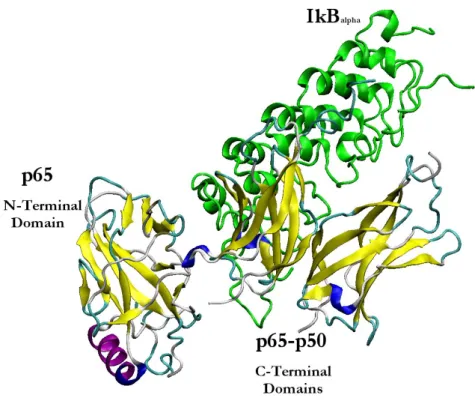
The metabolic regulation of NF-κB biological functions involves several control levels, one of the most important being in the interaction with proteins belonging to the IκB family in the cytoplasm. Among those, IκBα plays an inhibitory role, generating a complex with the inactive and resting state form of NF-κB homo- or hetero-dimers; this molecular interaction prevents NF-κB from translocating to the nucleus and exerts its regulatory functions on transcription of NF-κB target genes. The effect of IκBα is counteracted by IκBβ, that is able to compete with IκBα in binding NF-κB, thus leading to NF-κB activation. In response to a variety of stimuli including physical and chemical stresses, cytokines, reactive oxygen intermediates and ultraviolet light, the latent cytoplasmatic NF-kB/IκB complex is activated by the I-κB Kinase (IKK) complex. IKK is formed by three distinct subunits: IKKα, IKKβ and IKKγ. In the classical or canonical pathway, activation of IKK complex leads to the phosphorylation by IKKβ of two specific serines near the N terminus of IκBα, which targets IκBα for ubiquitination and degradation by the 26S proteasome. The unmasked NF-κB can then enter the nucleus and binds to the DNA target elements present in the promoters of NF-κB regulated genes, as well as to co-activators of gene transcription to activate target gene expression.

Moreover, cellular reducing catalyst thiredoxin (Trx) is a small endogenus molecule involved in NF-κB activation. Trx include in its structure a characteristic active site amino acid sequence, Cys-Gly-Pro-Cys able to reduce disulfide bonds.75 Some studies reported in literature shown that for the binding of NF-κB to the kB DNA, the cysteine residues must be in the reduced state.76,77 The DNA binding region of NF-κB p50 comprises a specific sequence composed by three arginine residues and a cysteine (Cys62) that is in oxidable state in cytoplasmatic cellular compartment condition. Thus, Trx recognizes and reduces NF-κB disulfide bond involving Cys62 in the nucleus allowing the protein/DNA complex formation, even if this binding process in vivo is not yet clarify.

(32)

2.3.1 Inhibitors of NF-κB and its dependent biological functions.

Based on the different molecular targeted approaches aimed at inhibition of NF-κB dependent biological functions78, the inhibitory molecules described in literature can be divided in the following classes:

1. Anti-oxidants that have been shown to inhibit activation of NF-kB 2. Proteasome and proteases inhibitors that inhibit Rel/NF-kB

3. IkBa phosphorylation and/or degradation inhibitors 4. Miscellaneous inhibitors of NF-kB

5. DNA mimics (NF-κB PNA-DNA chimeras) that bind NF-kB79

Several experimental model system are available for biological validation of molecules inhibiting NF-κB function. In this respect, transcription factor (TF) decoy strategy, based on inhibition of the binding of TF-related proteins to the consensus sequences present in the promoter of specific genes, demonstrated to modulate gene expression in vitro80,81 and in vivo.82,83 For example in cystic fibrosis (CF), several approaches can be followed, such as the identification by electrophoretic mobility shift assay (EMSA) of transcription factors activated by P. aeruginosa infection and their putative consensus sequences in the promoters of genes activated by this pathogen in CF epithelial cells. This information will help in identifying putative target transcription factors. NF-κB is one of the transcription factors demonstrated to be involved in CF. Interestingly; NF-κB plays a crucial role in regulating the expression of genes induced during P. aeruginosa infection, including interleukin 8 (IL-8) and intercellular adhesion molecule 1 (ICAM-1). Accordingly, molecules targeting the NF-κB signal transduction pathway are expected to be active on IL-8 and ICAM-1 gene expression.84

Besides the importance of these data for the theoretical point of view, these evidences are of great interest for the practical point of view, suggesting this treatment as a possible strategy for the therapy of inflammation associated with cystic fibrosis.85

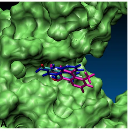
Target inactivation of NF-κB by directly binding to the p50 subunit is an important point of action of structurally different known inhibitor molecules86-92 such as Andrographolide and Selencotyanates that form covalent adducts with Cys-62 of p50. Recent studies have shown that p50 subunit of NF-κB is the one that mainly interacts with HIV-1 long terminal repeat.

(33)

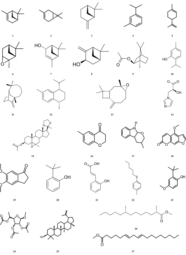
Interestingly, κB site-dependent transcriptional activation by homodimer p50 has been demonstrated in vitro.93 In particular, homodimers p50 specifically stimulated transcription from the immunoglobulin κ-site (equivalent to the HIV-1 enhancer site). Aurintricarboxylic acid (ATA) analogues (e.g., Bromopyrogallol Red, 1i; Pyrogallol Red, 2i; Pyrocatechol Violet, 3i) and polyhydroxycarboxylate derivatives (e.g., Gallic Acid, 4i; 5,7-dihydroxy-4-methylcoumarin, 5i; 7,8-dihydroxy-4-5,7-dihydroxy-4-methylcoumarin, 6i) have been reported as not-covalent inhibitors of NF-κB-p50-DNA binding (IC50 < 500 µM). 1i is the most active compound of

the series considered with a IC50 = 30 µM. Unlike, ATA (1n), ATA analogues (e.g., Aurin,

2n; Chrome Azurol S, 3n; Eriochrome Cyanine R, 4n; Fluorescein, 5n) and N,N' -[4-(dimethylamino)-2,6-pyridinylidenedimethyl] bis (S,S) (histidine)-di-methylester (6n) have been accounted as inactive ( IC50 > 500 µM) ligands94,95 (see Table 1).

(34)

NF-κB p50 binders (IC50 < 500 µM) O O H Y X X O R1 Y X O H Y R4 R3 R2 R1 X O Y 1i,2i 3i X Y R1 X Y R1 R2 R3 R4 1i OH Br _SO3H 3i _{OH H SO3H} H H H 2i OH H _SO3H O H O H OH CO₂H O O H O CH₃ X Y 4i 5i, 6i X Y 5i H OH 6i OH H

(35)

NF-κB p50 binders (IC50 > 500 µM) X O H Y R4 R3 R2 R1 X O Y O O H Y X X O R1 Y 1-4n 5n X Y R1 R2 R3 R4 X Y R1

1n COOH H H COOH OH H 5n H H COOH

2n H H H H OH H 3n COONa CH3 Cl SO3Na H Cl 4n COONa CH3 SO3Na H H H N N N N H H O O O O N N N N H H 6n Table 1. Chemical structures of known p50 binders

(36)

2.3.2 General structure features of NF-κB

The X-ray crystallographic structures of several Rel/NF-κB dimers on DNA (including p50-p50, p65-p65, p50-p65, c-Rel-c-Rel) have now been solved.96-101 These proteins share high sequence identity over a 300 amino acid 'rel homolgy region' (RHR) in the amino terminus. The RHR is responsible for protein dimerization, DNA binding, and nuclear localization. The 3D structure of the highly variable C-terminal domains (not present in p50 and p52) that contain transactivation domains (Tds) have not been solved.

2.3.2.1 NF-κB p50 homodimer bound to a kB site

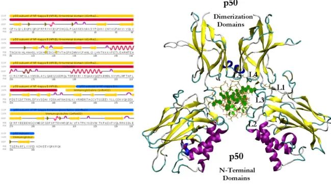
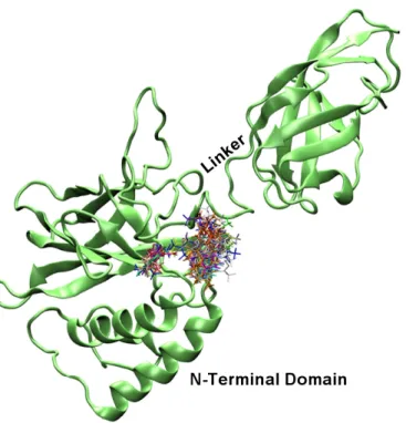
A crystal structure of 2.3 Ǻ of the NF-κB p50 homodimer bound to a 10-base-pair idealized palindromic kB site (PDB id: 1NFK) has been solved by Ghosh et al.97 The protein is derived from mouse and contain residues 39-364 including the entire RHR essential for DNA binding for each truncated p50 subunit (see Figure 2).

The homodimeric p50 binding site (5'-TGGGAATTCCC-3'; 3'-CCCTTAAGGGT-5') is derived from the consensus sequences of intronic enhancer element of kB light chain (Ig-kB), human β-interferon gene enhancer κB site (β-IFN-κB) and major histocompatability class 1κB element (H2-κB). The 3D structure of p50 subunit consists of two immunoglobulin-like domains: the carboxyl-terminal dimerization domain (domain 1: 39-240) containing the basic nuclear localization sequence (NLS), and the DNA-binding amino-terminal domain (NTD, domain 2: 248-350). These two domains are connected by a 10 residues flexible linker (238-247). The “butterfly” open conformation of the protein encloses the cylindrical body of DNA. The DNA-protein recognition surface involves the flexible linker and well defined 5 loops that connect the β-strand for each p50 subunit and buries 3.55 A2_{of solvent accessible water.}

In particular, DNA base-specific contacts are created by loops coming from the amino-terminal domain, while non specific DNA ribo-phospate backbone interactions involved loop amino acids from both the amino-terminal and dimerization domain (see figure 2).

(37)

Figure 2. Structure of NF-kB p50-p50: (left) sequence of RHR of mouse p50 chain A. CATH and SCOP domain

assignment, DSSP secondary structure (5 helices - 41 residues; 27 strands - 101 residues) are highlighted; (right) three dimensional structure of the protein bound to DNA. The loops (L1-L5) of p50 subunit that contact DNA are shown.

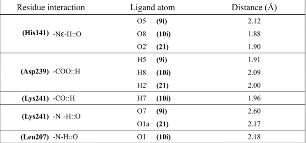
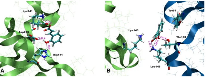
Most of the interacting residues highlighted in the figure above, have been confirmed by mutational analysis. Tyr57, Cys59 and Thr143, His64 may be involved in additional significant van der Walls contact in addition to hydrogen bonds to an extended DNA target. The contacts between the sugar-phosphate backbone and Cys59 account for the sensitivity of DNA binding to oxidation at this site.

The presence of Tyr57 in the central of the DNA/protein interface create from L1 explains its photochemical cross linking to DNA targets. Domain 1 includes 30 residues present only in p50 RHR sequence that access the DNA from the minor groove site. In particular the central phosphates form highly polarized strong hydrogen bonds with the sides chain of Lys144 and Lys145 and the NH of Lys144 backbone.

2.3.2.2 NF-κB p50-p65 heterodimer bound to a kB site

The overall topology of the NF-κB p50-p65 heterodimers is concordant with the structures of p50-p50 and other dimers crystallized on kB DNA targets. The 3 Ǻ protein crystal structures