An insight into the role of magnetic anisotropies in the behavior of thin films and arrays of nanoparticles

Università degli Studi di Ferrara

DOTTORATO DI RICERCA IN

"FISICA"

COORDINATORE Prof. Vincenzo Guidi

An insight into the role of magnetic anisotropies in the

behavior of thin films and arrays of nanoparticles

Settore Scientifico Disciplinare FIS/03

Dottorando Tutore

Dott. Fin Samuele Prof. Bisero Diego

Contents

INTRODUCTION ... 1

THEORETICAL CONCEPTS ... 3

Introduction ... 3

Magnetic Anisotropy ... 5

Domains and magnetic configurations ... 22

Reversal of Magnetization ... 27

Particle interaction ... 28

Spin Waves ... 29

The Micromagnetic modeling ... 31

EXPERIMENTAL METHODS ... 32

Introduction ... 32

Magnetic Force Microscopy ... 32

Magneto-Optical Kerr Effect ... 43

Vibrating Sample Magnetometer (VSM) ... 52

The Brillouin light scattering ... 54

THIN FILMS WITH PERPENDICULAR MAGNETIC ANISOTROPY: STRIPE DOMAINS AND “ROTATABLE ANISOTROPY” ..56

IRON-GALLIUM ... 57

Introduction ... 57

FeGa film production and characteristics ... 58

Magnetic Characterization ... 59

Rotatable Anisotropy in FeGa thin films ... 63

Comparison between BLS and MFM ... 70

Rotation and Reversal Processes ... 71

Bubble Domains Formation ... 77

Conclusions ... 83

TERBIUM-IRON-GALLIUM ... 85

Introduction ... 85

Production of TbFeGa Thin Films ... 85

MFM and MOKE measurements ... 90

ARRAYS OF MAGNETIC NANOPARTICLES: “CONFIGURATIONAL ANISOTROPIES” ...99

BICOMPONENT ELLIPSES (CO/PY,PY/NI):CONFIGURATIONAL ANISOTROPY ... 100

Introduction ... 100

Bicomponent Co/Py ... 102

Bicomponent Py/Ni... 113

FINITE ARRAYS OF PY DISKS: GLOBAL CONFIGURATIONAL ANISOTROPY ... 120

Introduction ... 120

Samples Fabrication ... 121

Circular Dot Arrays ... 122

Conclusions ... 141

CONCLUSIONS ... 142

1

Introduction

In the last years the scientific interest on nanotechnologies has covered all the research fields, starting from electronics and magnetism due to the necessity to reduce the sizes of hardware in computers and increase the density of memory storage.

The importance of studying the magnetic properties of nanostructures derives from the fact that they change dramatically when the dimensions are reduced under the micrometer and new physical phenomena take place. With respect to the bulk magnetic materials, effects like Giant Magnoresistance, Oscillatory Exchange Coupling or Perpendicular Magnetic Anisotropy (just to quote some examples) are evidenced and they have a great impact on the development of new technological equipment and products.

The reasons of the different magnetic behavior of the materials when they are in the nanostructured form must be searched primarily in the change of the relative strength of dipolar and exchange interactions and in the elemental (and then) quantum-mechanical nature of the matter, which emerges when the dimensions of the objects are near to those of the atom itself. One of the important properties which is strongly affected by the size reduction and in which is contained most of the physical description of a magnetic system is the anisotropy energy term: a direction-dependent parameter which strongly contributes to the determination of the equilibrium state and magnetic behavior.

In this thesis we describe various nanostructured systems concentrating prevalently on thin films and arrays of interacting nanoparticles and for each system the origin and the physical implications of magnetic anisotropy is discussed.

In the first chapter we report the theoretical knowledge of nanomagnetism: the energy terms involved in the determination of equilibrium state and reversal process, various typologies of

2

magnetic anisotropies, their origins and their implications. We perform a description of the magnetic domains and how they are influenced by the shape and dimensions of the nanoparticles. In the second chapter a brief discussion of the experimental instrumentation is done. We report the experimental methods and instrument prevalently used: Magnetic Force Microscopy for the determination and imaging of the magnetization distribution, the Magneto-Optical Kerr Effect Magnetometry and Vibrating Sample Magnetometer for the production of the hysteresis loops and finally the Brillouin Light Scattering technique for the detection of the spin-wave frequencies in the magnetic media.

The following part of the thesis deals with the nanostructured systems analyzed and anisotropies characterizing them. It is divided in two sections: thin magnetostrictive films and arrays of nanoparticles.

In the first topic, two types of magnetic anisotropies are presented: Perpendicular Magnetic Anisotropy which has a crystalline origin and competes with the shape anisotropy of the thin film producing a singular type of magnetic domains called “stripes” and the Rotatable Anisotropy (the easy magnetic direction is not fixed but could be rotated by means of an external magnetic field). We tried to give a better explanation and modeling of the Rotatable Anisotropy, making a parallelism between the static and dynamic experimental evidences.

The second topic regards the description of the interaction of magnetic dots in arrays with different symmetry and with finite dimensions. In particular we discovered a peculiar space-dependent behavior that we called “global configurational anisotropy”, that has a strong importance when the dimension of the array becomes comparable with the dimension of the nanoparticles.

3

Theoretical Concepts

Introduction

The “Nanomagnetism” is the area of research in physics that refers to the magnetic properties and behaviors of systems in which at least one of the spatial dimensions is reduced in the nanoscopic scale. Nanomagnetism involves objects like films (one dimension is in the nanoscale), nanowires (two dimensions are in the nanoscale) and nanodots (all the spatial dimensions are in the nanoscale).

It is possible to combine magnetic and non-magnetic films in multilayers, superimposing one film to the other, as it is possible to bring the nanowires so close that they interact (1) and even to produce nanowires multilayered (2). Moreover it is possible to form one-dimensional (chains) and two-dimensional arrays of nanodots, single or multi-layered, and for each arrangement the dots could have different dimension, composition or geometry (circular, squared, exagonal etc.) (3). All the infinite combinations of dimensionality, size, shape, composition, interaction, symmetry give as many different magnetic properties like equilibrium energies, domain shapes, switching fields, coercive fields or the dynamical responses of the spin-wave frequencies. Every features change, as we will see, could be associated to an anisotropy term, that is an energy term whose minimization could be reached only in some particular directions of the system.

To better structure and frame the following considerations on magnetic behaviors and magnetic anisotropies involved in the studied systems we do a brief theoretical excursus on the general knowledge of magnetism and then we relate it with the reduction of dimension in magnetic materials in the specific sections.

4

The magnetostatic energy

The magnetostatic energy arises from the interaction of the magnetization itself with the magnetic field Hd i.e. the field coming only from any divergence in the magnetization M. This is the reason

why this term is also said “self energy”. The magnetostatic energy density can be expressed in the following term:

0

2

ms

E

 



H M



In a magnetic body in equilibrium, the demagnetizing field H is antiparallel to the magnetization d

that generates it.

The exchange energy

The exchange energy is a quantum mechanical quantity that can be described by a phenomenological approach. Considering the following expression:

2

_cos

E

JS



 



where S is the total spin momentum per atom and  is the angle between the directions of the ij

spin momentum vectors of atom i and j, the term J is the exchange constant, which is a measure of the intensity of the interaction. The exchange constant, or exchange integral, comes from the quantum mechanical interaction between electrons in their shared orbitals. In ferromagnetic materials the exchange integral is positive and thus the energy is minimized when the spins are parallel. From this point of view, the exchange energy is in competition with the magnetostatic energy and the equilibrium point is determined by the shape, size and thickness of the object. (4)

5

The Zeeman energy

The Zeeman contribution to the overall energy is due to the application of an external magnetic field:

0

Z

E

 



M H



The Zeeman energy is minimized when the magnetization is aligned with the external field (as we can see from the fact that the scalar product reaches its maximum when the magnetization vector is parallel to the external field).

The anisotropy energy

When a physical property of a material is a function of direction, that property is said to exhibit anisotropy. The preference for the magnetization to lie in a particular direction in a sample is called Magnetic Anisotropy.

There are different sources of the anisotropy: shape, magnetocrystalline, surface and interface anisotropy, strain anisotropy and growth induced anisotropy, configurational anisotropy etc. Each type of energy term contribution modifies the total amount of energy density and therefore the magnetic behavior of the material and in particular we will see as magnetic anisotropy could influence the magnetic properties of a system.

Magnetic Anisotropy

Shape Anisotropy

The shape anisotropy is due to the presence, in every magnetic sample, of a demagnetizing field

d

H which opposes to magnetization and tends to reduce it prevalently in the direction in which it has a greater value.

6

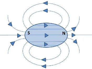
Suppose a bar sample is magnetized by a field applied from left to right and subsequently removed. Then a north pole is formed at the right end, and a south pole at the left, as shown in Fig. 1 (5). We see that the H lines, radiating out from the north pole and ending at the south pole, constitute a field both outside and inside the magnet which acts from north to south and which therefore tends to demagnetize the magnet.

Figure 1: Emergent surface stray field and bulk demagnetizing field due to the “free poles” at the edges of a magnetized bar.

This self-demagnetizing action of a magnetized body is important, not only because of its bearing on magnetic measurements, but also because it strongly influences the behavior of magnetic materials in many practical devices.

The demagnetizing field H acts in the opposite direction to the magnetization M which creates it. d

If we model the shape of the bar, smoothing its corner, it is possible to obtain a ideally uniform parallel demagnetizing field. It may be shown, although not easily, that the correct taper to achieve this result is that of an ellipsoid (Fig. 2) (5). If an unmagnetized ellipsoid is placed in a uniform magnetic field, it becomes magnetized uniformly throughout; the uniformity of M and B are due to the uniformity of Hd throughout the volume. This uniformity can be achieved only in an

7

Figure 2: Uniform magnetization and uniform demagnetizing field in an ellipsoid.

The demagnetizing field Hdof a body is proportional to the magnetization which creates it and as

said is antiparallel: Hd =-NdM

where Nd is the demagnetizing factor or demagnetizing coefficient.

The value of Nd depends mainly on the shape of the body, and has a single calculable value only

for an ellipsoid.

It is clear that it depends on the relative lengths of the three spatial dimensions: along a short axis the external surfaces are very close and this favors the demagnetization, and therefore the demagnetizing factor increases; viceversa, in a long axis the surfaces (and thus the “free magnetic charges”) are not close and it is more difficult to demagnetize the sample in that direction. The sum of the demagnetizing factors along the three orthogonal axes of an ellipsoid is a constant. Na + Nb + Nc = 1

For a sphere, the three demagnetizing factors must be equal, so Nsphere =1/3.

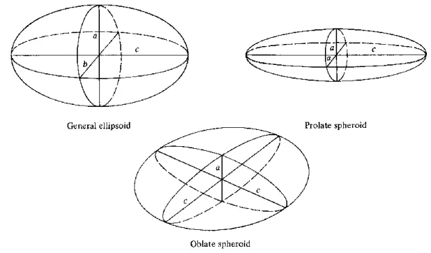
The general ellipsoid has three unequal axes 2a, 2b, 2c, and a section perpendicular to any axis is an ellipse (Fig. 3) (5). Of greater practical interest is the ellipsoid of revolution, or spheroid. A

8

prolate spheroid is formed by rotating an ellipse about its major axis 2c; then a = b < c, and the resulting solid is cigar-shaped. Rotation about the minor axis 2a results in the disk-shaped oblate spheroid, with a < b = c. Maxwell calls this the planetary spheroid, which may be easier to remember (5).

Figure 3: Ellipsoids with different ratio between the axis. General, Prolate (Cigar) and Oblate (Planetary) spheroids.

Equations, tabular data, and graphs for the demagnetizing factors of general ellipsoids are given by E. C. Stoner [Phil. Mag., 36 (1945) p. 803] (6) and J. A. Osborn [Phys. Rev., 67 (1945) p. 351] (7). Specimens often encountered in our practice are thin films, elliptical dots or disks magnetized in their plane.

What is important to evidence is that the contribution to the Magnetostatic Energy is strictly conditioned from the shape of the sample.

In the next section we will see in particular three types of systems: thin films, nanostructured ellipses and circular nanostructured dots. We can to some extent represent thin films as oblate spheroid (as in figure 3) with a→0 and b = c both very large. We see as for thin film Na≈1, Nc→0.

9

For circular disk the situation is not trivial and each case must be considered individually. Finally for the elliptical dots, we can consider the case of a general spheroid but it is simple to show how the easy direction is everytime the longer one.

Consider a polycrystalline specimen having no preferred orientation of its grains, and therefore no net crystal anisotropy. If it is spherical in shape, the same applied field will magnetize it to the same extent in any direction. But if it is nonspherical, it will be easier to magnetize it along a long axis than along a short axis. The reason for this is (as clearly described just now) the demagnetizing field along a short axis is stronger than along a long axis. The applied field along a short axis then has to be stronger to produce the same true field inside the specimen. Thus shape alone can be a source of magnetic anisotropy.

In order to treat shape anisotropy quantitatively, we write an expression for the magnetostatic energy Ems of a permanently magnetized body in zero applied field. If a body is magnetized by an

applied field to some level A (Fig.4) (5) and the applied field is then removed, the magnetization will decrease to C under the action of the demagnetizing field Hd.

Figure 4: the applied field is then removed, the magnetization will decrease under the action of the demagnetizing field Hd. The

shadowed area is the magnetostatic energy of the magnet.

Here OC is the demagnetizing-field line, with a slope of -1/Nd, where Nd is the demagnetizing

10

OCD. This energy is that associated with the demagnetizing field of the specimen, and is variously called the magnetostatic energy, the self-energy, or the energy of a magnet in its own field.

where dv is an element of volume and the integration extends over all space. The distribution of Hd in space is generally not known accurately and, even when it is, the evaluation of this integral

would be difficult. It is easier to compute the area of the triangle OCD in Fig.4. This energy can be written in vector form as

0

2

ms

E

 



H M



where M is the level of magnetization at point C.

Since magnetization and demagnetizing field vectors are antiparallel H_d  N_dM therefore (in the SI) 2 0

2

E





N M

In BCC Fe, the magnetization process is said to be easy in the [100] directions and hard in the [111] directions because the field needed to magnetize iron to saturation is smaller in the [100] direction than in any others. This is called Magnetocrystalline Anisotropy because its origin is of crystalline structure nature and could be explained considering the Spin-Orbit coupling in the atoms of the ferromagnetic material. In FCC Nichel, the case is just the opposite: [111] directions are easy, [100] hard, and the fields required for saturation in the hard directions are smaller for Ni than for Fe. Cobalt is hexagonal, and its easy direction of magnetization is the c axis; to saturate

2 0

2

ms d

11

the sample in the basal plane is very difficult, more than an order of magnitude harder than in the [111] directions in Fe.

After saturation, reduction of the field to zero leaves most of the magnetization remaining in the direction in which the field had been applied if it is an easy direction. In the absence of an external field, the magnetization remaining at H=0, called “remanence”, is non zero for Fe and Ni magnetized in hard directions, whereas it is zero for Co magnetized in a hard direction.

12

Figure 5 shows that fairly high fields, of the order of several hundred Oersteds, are needed to saturate iron in a [110] direction.

More generally, the direction of easy magnetization of a crystal is the direction of spontaneous domain magnetization in the demagnetized state. When an increasing external field is applied to one arbitrary direction, the magnetization grows in the easy direction following the scheme of figure 6 (5).

Figure 6: an increasing external field is applied away from the easy direction. The domain walls move and favor the domains with a component of magnetization along the field, reducing the dimensions of the other (b). When the domains are saturated in the easy

directions, the spins rotate along the field direction (d).

Domain wall motion, in a low field, occurs until there are only two domains left (Fig. 6c), each with the same potential energy. The only way in which the magnetization can increase further is by rotation of the Ms vector of each domain until it is parallel with the applied field. This process is

called domain rotation. The domain itself, which is a group of atoms, does not rotate. It is the net magnetic moment of each atom which rotates. Domain rotation thus happens at very high field due to the magnetocrystalline anisotropy, this “force” which works to leave the magnetization in a specific direction.

13

When the rotation process is complete (Fig. 6d), the domain wall in Fig. 6c disappears, and the crystal is saturated.

Due to the fact that the domain rotation spends a certain amount of energy to be performed, there should be a great amount of energy stored in the material when the magnetization is not in the easy direction and this is called “crystal anisotropy energy”.

The Russian physicist Akulov showed in 1929 that this energy can be expressed in terms of a series expansion of the direction cosines of Ms relative to the crystal axes. In a cubic crystal, let Ms

subtends angles a, b, c with the crystal axes, and let α1, α2, α3 be the cosines

of these angles, which are called direction cosines. Then









0 1 1 2 2 3 3 1 2 1 2 3

..

E K





K

 



 



 



K

  



where K0, K1, K2, . . are constants for a particular material at a particular temperature and are

expressed in erg/cm3(cgs) or J/m3(SI). Higher powers are negligible, and sometimes K2is so small

that the term involving it could be ignored. The first term, K0, is independent of angle and is

usually skipped, because normally we are interested only in the change in the energy E when the Ms vector rotates from one direction to another. For example in a bcc crystal ifK1 is positive, then

E100 < E110 < E111, and [100] is the easy direction, because E is a minimum when Msis in that

direction.

In the hexagonal Cobalt there is a unique easy axis and the other direction are equivalently hard. We speak of Uniaxial Anisotropy and the Akulov formula could be simplified as

2 4

0 1

sin

sin

..

E K





K





K





Where θ is the angle between the magnetization and the c axis of the hexagonal structure.

When K1 and K2 are both positive, the energy E is minimum for θ = 0, and the c-axis is an axis of

14

either up or down, is referred to as a uniaxial crystal, as noted above. Its domain structure in the demagnetized state is particularly simple (figure 7). Elemental cobalt, barium ferrite, and many rare earth transitional metal intermetallic compounds behave in this way.

Figure 7: magnetization breaks in domains in uniaxial anisotropy crystals.

Crystal anisotropy is due mainly to spin-orbit interaction. The orbit of the electron is strongly linked to the lattice configuration. There is also a coupling between the spin and the orbital motion of each electron. When an external field tries to reorient the spin of an electron, the orbit of that electron also tends to be reoriented. But the orbit is strongly coupled to the lattice and therefore resists the attempt to rotate the spin axis. The energy required to rotate the spin system of a domain away from the easy direction, which we call the anisotropy energy, is just the energy required to overcome the spin–orbit coupling. Inasmuch as the “lattice” consists of a number of atomic nuclei arranged in space, each with its surrounding cloud of orbital electrons, we can also speak of a spin–lattice coupling and conclude that it too is weak. These several relationships are summarized in Fig. 8 (5)

15

Figure 8: Spin-orbit coupling scheme.

The magnitude of the crystal anisotropy generally decreases with temperature more rapidly than the magnetization, and vanishes at the Curie point. Since the anisotropy contributes strongly to the coercive field, the coercive field generally goes to zero together with the anisotropy.

Anisotropy Field

The crystal anisotropy forces which hold the spontaneous magnetization Ms of any domain in an

easy direction can also be expressed in an indirect but often useful way that doesn’t make use of anisotropy constants. For small rotations of the magnetization away from an easy direction, the crystal anisotropy acts like a magnetic field trying to hold the magnetization parallel to the axis. This field is called the anisotropy field and is given the symbol HK. The anisotropy field is parallel to

the easy direction and its magnitude, for small angular deviations θ, exerts the same torque on Ms

as the crystal anisotropy itself. The torque due to the anisotropy field is H M_{K s}sin, or H M_{K s} for small values of θ. For example, in a cubic crystal with [100] easy directions, the torque exerted on Msby the crystal when Ms rotates away from [100] is, K1/ 2sin 4, or 2K1 for small θ. Equating these torques, we have

1

2

16 1

2

K

H

M



2

K

H

M





This is the expression for the Anisotropy Field in the case of magnetocrystalline anisotropy. As we will see in the next chapters it could be associated not only to magnetocrystalline anisotropy but extended to the other type of magnetic anisotropies.

Induced Anisotropy

Stress effects

When a substance is exposed to a magnetic field, its dimensions change. This effect is called magnetostriction. It was discovered in 1842 by Joule, who showed that iron in bulk form increased its length when it was magnetized lengthwise by a weak field (5).

The fractional change in length l

l



is simply a strain, and, to distinguish it from the strain ε caused

by an applied stress, we give the magnetically induced strain a special symbol:

l l



The value of λ measured at magnetic saturation is called the saturation magnetostriction λs, and,

when the word “magnetostriction” is used without qualification, λsis usually meant. The origin of

17

Figure 9: magnetostriction is caused by the rotation of the orbit around the nuclei.

The black dots represent atomic nuclei, the arrows show the net magnetic moment per atom, and the ellispoidal lines enclose the electrons in a fixed orbit around the nuclei in the magnetostrictive crystal. The upper row of atoms depicts the paramagnetic state above Tc. If, for the moment, we

assume that the spin–orbit coupling is very strong, then the effect of the spontaneous magnetization occurring below Tc would be to rotate the spins and the electron clouds into some

particular orientation determined by the crystal anisotropy. The nuclei would be forced further apart, and the spontaneous magnetostriction would be 0

0

l l 

. If we then apply a strong field

vertically, the spins and the electron clouds would rotate through 90 degrees, and the domains

strain by an amount l

l

 .

Thus an applied mechanical stress can alter the domain structure and create a new source of magnetic anisotropy. These effects can have a substantial influence on the low-field magnetic properties, such as permeability and remanence.

The saturation magnetostriction λsi of a cubic crystal in a direction could be expressed as a

18

changes from the demagnetized state to saturation in a direction defined by the direction cosines α1, α2, α3, and is given by





where λ100 and λ 111 are the saturation magnetostrictions when the crystal is magnetized, and the

strain is measured, in the directions [100] and [111], respectively.

The symbol σ will be used here and in the following paragraphs for applied mechanical stress. H, M (or B), and σ could be all parallel, but, in general, M and σ may not be parallel. We know from the previous equation that the amount of magnetostrictive strain exhibited by a crystal in a particular direction depends on the direction of the magnetization. If we impose an additional strain by applying a stress, for the Villari effect we expect that the direction of the magnetization will change. We therefore need a general relation between the direction of M within a domain and the direction and magnitude of σ. But we know that, in the absence of stress, the direction of M is controlled by crystal anisotropy, as characterized by the first anisotropy constant K1. Therefore,

when a stress is acting, the direction of M is controlled by both σ and K1. These two quantities are

therefore involved in the expression for that part of the energy which depends on the direction of M, which is, for a cubic crystal













Where α1, α2, α3 are the direction cosines of M, as before, and 1, 2, 3 are the direction cosines of the stress σ. The equilibrium direction of Ms is that which makes E a minimum, and this

direction is seen to be a complicated function of K1, λ100, λ111, and σ, for any given stress direction

γ1, γ2, γ3 .

Stress alone can create an easy axis of magnetization. Therefore, when stress is present, stress anisotropy must be considered. It is a uniaxial anisotropy, and the relation which governs it, is of

19

exactly the same form as for uniaxial crystal anisotropy or shape anisotropy. We therefore write for the stress anisotropy energy, which is a magnetoelastic energy

2

sin

me

E



K



Configurational Anisotropy

It was demonstrated (3) that in a squared array of spins at least two different spatial configuration of the magnetization are equilibrium states of the magnetostatic energy.

Figure 10: Flower (a) and Leaf (b) magnetization configuration are equilibrium states, created by the application of a field along the side or along the diagonal of the squared dot. This effect is called “configurational anisotropy”.

It is possible (3) to model the flower and leaf (figure 10 a and b) states analytically as small perturbations from the uniformly magnetized state and find that the energy surface between the states can be described by a fourfold symmetric configurational anisotropy field which changes sign at a critical width to thickness aspect ratio. Figure 10 shows examples of equilibrium magnetization vector fields calculated for square nanostructures. Figure 10a shows the vector field (also called a configuration) which occurs when one magnetizes the structure parallel to one of its edges. This configuration is usually poetically named the ‘flower’ because of the way it flares out at the top and bottom, like the center of a daffodil. Figure 10b shows the configuration associated with a square magnetized along its diagonal. We name this configuration the ‘leaf’ because of the way that it bows out in the center and then nips together at the ends, like a plant leaf. The

20

numerical calculation of an equilibrium magnetization field can be repeated for each value of a varying applied field in order to simulate a hysteresis loop, or as a function of nanomagnet orientation in order to predict anisotropy values.

The concept could be extended to “array of dots” and the configurational anisotropy will assume a more wide significance, as we will describe in the second part of this thesis.

Other Anisotropies

Various other anisotropies may be induced in certain materials, chiefly solid solutions, by appropriate treatments. These induced anisotropies are of interest both to the physicist, for the light they throw on basic magnetic phenomena, and to the technologist, who may exploit them in the design of magnetic materials for specific applications (5).

The following treatments can induce magnetic anisotropy:

1. Magnetic annealing. This means heat treatment in a magnetic field, sometimes called a thermomagnetic treatment. This treatment can induce anisotropy in certain alloys. (Here the term “alloys” includes not only metallic materials but also mixed ferrites.) The results depend on the kind of alloy:

a. Two-phase alloys. Here the cause of anisotropy is the shape anisotropy of one of the phases and is therefore not basically new. However, it is industrially important because it affects the behavior of some of the alnico permanent-magnet alloys.

b. Single-phase solid-solution alloys

2. Stress annealing. This means heat treatment of a material that is simultaneously subjected to an applied stress.

3. Plastic deformation. This can cause anisotropy both in solid solutions and in pure metals, but by quite different mechanisms.

21

4. Magnetic irradiation. This means irradiation with high-energy particles of a sample in a magnetic field.

Exchange Anisotropy

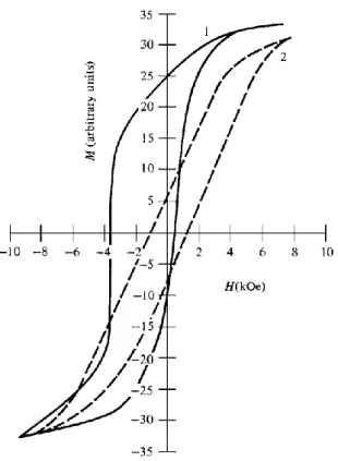
Another interesting small-particle effect was discovered in 1956 by W. H. Meiklejohn and C. P. Bean (8), who called it exchange anisotropy. They took fine, single-domain particles of cobalt and partially oxidized them, so that each cobalt particle was covered with a layer of CoO. A compact of these particles was then cooled in a strong field to 77K, and its hysteresis loop was measured at that temperature. This loop, shown by the full curve of Fig. 11, is not symmetrical about the origin but shifted to the left. If the material is not cooled in a field, the loop is symmetrical and entirely normal (dashed curve). The field-cooled material has another unusual characteristic: its rotational hysteresis loss Wr, measured at 77K, remains high even at fields as large as 16 kOe, whereas Wr

decreases to zero at high fields in most materials.

These two features of exchange anisotropy, a shifted loop and high-field rotational hysteresis, have been found in other materials, including alloys. For example, disordered nickel-manganese alloys at and near the composition Ni3Mn are paramagnetic at room temperature but show

22

Figure 11: Asymmetric/symmetric hysteresis loop for a sample cooled/not in a field due to the effect of exchange anisotropy.

Domains and magnetic configurations

In presence of a magnetization M, the magnetic field H can be split in two components, the applied field H and the magnetostatic field ext H , coming only from the magnetization d M. For

d

H the following equation is valid: H_d 0, given that j = 0. The most general solution is ( )

d U r

H . From the third Maxwell equation ( B 0), being B 0





substituting U r( ), it is obtained that U r( ) is solution of:   M2U . Considering the boundary conditions, the solution of the equation can be calculated:

1

'

( ')

( ')

( )

'

'

4

'

'

r

n

r

U r

d

d

r r



r r





_{ }

_





_

_





_

_













M

M

S

23

From the equation above two terms can be identified: a bulk term (M), that is zero when M is uniform everywhere and a surface term (n M· ), that is zero when Mis parallel to borders. When a high external field is applied so that the sample reaches a saturated state, uniform magnetization is favoured. At small magnetic field, the magnetization is generally arranged in order to reduce the magnetostatic energy.

The way to do so is formation of domains structure, where the magnetization is arranged in a closed flux circuit without leakage outside the material. In each magnetic domain the magnetization is homogenous and oriented parallel to one of the easy directions. At the interface between one domain and the next, the magnetic spins have to change their orientation. Into the material there are then regions, called domain boundaries, which are costly in terms of energy (4) (9). An excess of anisotropy and exchange energy is stored in domain boundaries, considering that within the wall each spin is misaligned slightly from its neighbours, against the exchange energy that will tends to align the adjacent spins. On the other hand, these same atomic spins within the wall do not lie parallel to an easy direction, so there will be an anisotropy energy associated with the wall presence. Summarizing, the number and the shape of domains are determined by the balance of three energy terms: the magnetostatic energy and the anisotropy and exchange energies associated with the walls. When the lateral size of the ferromagnetic structure becomes to be so small that is comparable with the domain wall dimension, the magnetization configuration becomes a single domain. If then the size becomes too small, the magnetic moment of the single domain ferromagnet can fluctuate, due to the thermal energy, and the object becomes superparamagnetic (10).

In the simple ideal case, it is assumed that the rotation of the magnetization inside the wall is always normal to the magnetization on both the domains separated by the wall. This is the case of

24

the Bloch wall domain. The energetic cost due to the presence of a domain wall can be evaluated as:

1

W

AK







where A is the exchange stiffness constant and α is a coefficient depending on the material, the type of boundary and the direction normal to the boundary.

Another type is the Néel wall domain: the magnetization rotates from the direction of the first domain to the direction of the second, with a rotation that is within the plane of the domain wall. It consists of a core with fast varying rotation and two tails where the rotation logarithmically decays. Néel walls are the common magnetic domain wall type in very thin film where the exchange length is very large compared to the thickness.

Figure 12: Bloch wall and Néel wall types.

Specific length-scales

Considering the example of a spherical object with radius R and constituted by a specific material (so that A and K1are known) and calculating the energy for the single domain state and for a two

25

domains state, the critical radius below which the former state is energetically stable can be written as (11): 1 sd 2 0

36

R

AK

M





The competition between exchange and dipolar energy can be expressed in terms of the exchange length lex (12):

2 0

2

A

l

M





which represents the spatial scale below which exchange dominates on the magnetostatic effects. Another important parameter is the hardness:

1 2 0

2

K

M







that measures the relative importance of anisotropy compared to magnetostatic effects. The domain wall width parameter

1 ex

l

A

K



 



is related to the domain wall width 0 is given by (12)

0

1

A

K







 



The relative values of the characteristic lengths change as a function of the degree of magnetic hardness of the materials. For soft magnetic materials, one has:

sd

R

  

l

26

sd

R

  

l

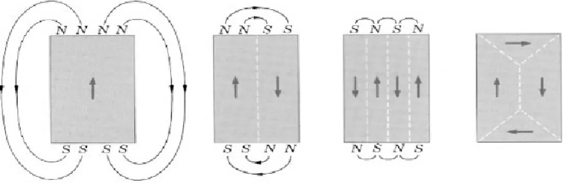
In the figure 13 (4) below we report some examples of magnetic domain structures in a rectangular ferromagnet. The magnetostatic energy is considerably reduced for the last two examples where a closure domain configuration is clearly visible.

Figure 13: single domain, multi-domains and examples of closure domains.

The circular shape has a strong potential for nanomagnets, due to its lack of shape anisotropy and configurational anisotropy. If the circular dot is constituted by an isotropic material, as it is for Py, it results that its magnetization can be changed in direction by a very weak applied magnetic field. It is just in the circular objects that it appears a particular closure domain: the magnetic vortex (13), in which the magnetization direction changes in the plane of the object, lowering the system energy by reducing the stray field. In the core the magnetization is perpendicular to the surface plane, so the only residual magnetostatic energy is confined in the center which could be seen as a topological singularity, that gives to the object two key properties: chirality (clockwise or counterclockwise rotation of magnetization) and polarity (positive or negative direction of the core magnetization). A scheme of the magnetization orientation in a vortex is represented in image 14.

27

Figure 14: magnetization distribution in a vortex. The topological singularity determines the polarity; the chirality indicates the rotation of the magnetization.

Reversal of Magnetization

When the particle lateral dimensions begin to be small, the single domain is energetically more favorable and the reversal nucleation field is greater in than the extended film. This means that the coercivity increases when the particle dimension is reduced. We report in figure 15 a scheme in which the coercivity as function of the particle dimension is summarized. We see that as we go from right to left (when we reduce the diameter of the particle) the coercivity increases.

28

Figure 15: as the dimensions of the particle are reduced, the single domain is favored and as consequence the coercive field grows. If the dimensions are still reduced, the thermal excitations misalign the spins in a chaotic distribution (superparamagnetic behavior)

and the coercive reduces to zero.

When the diameter of the particle is further reduced the coercivity starts to reduce and when the thermal energy is greater than the magnetic energy the particle becomes superparamagnetic due to the thermal excitations which misalign the spin orientation. The magnetization reversal process is energetically favored if it passes through a domain wall motion, but when the particle is single domain the nucleation field is still smaller than that for coherent reversal. Two different mechanism of incoherent spin rotation, the magnetization buckling and magnetization curling, are now energetically favoured as sketched in Figure 16 (14).

Figure 16: coherent rotation, curling and buckling reversal mechanism.

Particle interaction

In a magnetic nanodots array the only interaction between the particles is the dipolar interaction (or dipolar coupling) that acts in the long range, because its magnitude scales as r3

It derives from the magnetic dipole-dipole interaction which would favor the alignment of the magnetization of a particle to the stray-closure flux produced by the neighbor particle. In figure 17

29

it is simply sketched the dipolar influence of the uniformly magnetized particle A on the particle B and C.

Figure 17: coupling interactions between magnetic particle.

The particle C tends to be magnetized antiparallel to A, while the particle B prefers a magnetization in the same versus of the particle A.

For circular magnetic dots in an array the coupling interaction favors vortexes with identical chirality and polarity (15).

It is not trivial to understand how the coupling interaction affect the reversal process in a magnetic dot array for different dimensions and relative dispositions, but it was one of the objective of the work done.

Spin Waves

Spin waves are propagating disturbances in the ordering of magnetic materials. These collective excitations occur in magnetic lattices with continuous symmetry. From the equivalent

30

quasiparticle point of view, spin waves are known as magnons, which are boson modes of the spin lattice that correspond roughly to the phonon excitations of the nuclear lattice. As temperature is increased, the thermal excitation of spin waves reduces a ferromagnet's spontaneous magnetization. The energies of spin waves are typically only μeV. Spin waves can propagate in magnetic media with magnetic ordering such ferromagnets and antiferromagnets. The frequencies of the precession of the magnetization depend on the material and its magnetic parameters; in general precession frequencies are in the microwave from 1–100 GHz, exchange resonances in particular materials can even see frequencies up to several THz. This higher precession frequency opens new possibilities for analogue and digital signal processing.

Spin waves themselves have group velocities on the order of a few km per second. The damping of spin waves in a magnetic material also causes the decay of amplitude of the spin wave with distance, meaning that the spin waves can travel usually only several 10's of μm. The damping of the dynamical magnetization is accounted by the Gilbert damping constant in the Landau-Lifshitz-Gilbert equation (LLG equation).

The LL equation was introduced in 1935 by Landau and Lifshitz to model the precessional motion of magnetization M in a solid with an effective magnetic field Heff and with damping. Later, Gilbert

modified the damping term, and in the limit of small damping yields the older LL equation. The LLG equation is,

(

)

M

t

M







 







M × H

M

M × H

The constant α is the Gilbert phenomenological damping parameter and depends on the solid; γ is the electron gyromagnetic ratio.

A magnonic crystal is a magnetic meta-material with alternating magnetic properties. Like conventional metamaterials, their properties arise from geometrical structuring, rather than their

31

band-structure or composition directly. Small spatial inhomogeneities create an effective macroscopic behavior, leading to properties generally not found in nature. By alternating parameters such as the relative permeability or saturation magnetization, there exists the possibility to tailor 'magnonic' bandgaps in the material. By tuning the size of this bandgap, only spin wave modes able to cross the bandgap would be able to propagate through the media, leading to selective propagation of certain spin wave frequencies (16).

The Micromagnetic modeling

The full quantum mechanical approach is used when the dimensions of the nanostructures are of the order of atoms and molecules, while in the mesoscopic range phenomenological constants (i.e. the exchange constant, anisotropy fields) are introduced.

In the mesoscopic scale a classical approximation of the description of the magnetic materials called “micromagnetic approach” is introduced and the discrete nature of the matter is neglected. In the micromagnetic theory the total free energy is a result of several terms, whose balance determines the magnetic properties of the system. In physics (and therefore in this theory) a system in equilibrium is in a local minimum of the total free energy. If thermal fluctuations are not considered, i.e. the system is at 0 K, this can be written as:

Etot = Ed + Eex + EZ + Eanis

where Ed is the magnetostatic energy, Eex is the exchange energy, EZ is the Zeeman energy and

Eanis is the anisotropy energy. The determination of the exact values of all these terms, and in

particular the condition under which they are in a local minimum, allows us to predict the magnetic behavior of the considered system.

32

Experimental Methods

Introduction

The present thesis work concerns an experimental analysis and characterization of some novel nanostructured systems: FeGa (produced by the group of Prof. Marangolo at the University Pierre et Marie Curie in Paris) and TbFeGa (produced by Rocio Ranchal at University Complutense in Madrid) in thin films, bicomponent array of ferromagnetic ellipses (done by the group of prof Adeyeye at University of Singapore) and finite-size array of Py nanodots (by the group of Vavassori at Cic Nanogune in San Sebastian, Spain).

The main methods for detection of the magnetic properties were Magnetic Force Microscopy, for the determination and visualization of the magnetization configuration, the Magneto-Optical Kerr Effect Magnetovectometry for the determination of the variation of magnetization under the field application in the three spatial directions, the Vibrating Sample Magnetometer and finally the Brillouin Light Scattering for the analysis of the spin-wave frequencies. MFM and MOKE are measurements performed with instruments at the University of Ferrara, VSM at the UPMC while BLS is performed at the Department of Physics and Geology of the University of Perugia.

Magnetic Force Microscopy

The Magnetic Force Microscope is a type of Scanning Probe Microscope. The principle of operation is based on the scheme reported in the image 1 (17).

33

Figure 1: scheme of the principle of operation of SPM.

A laser beam is focused over a reflecting “cantilever” which is suspended on one side. On the free end a small volume of magnetic material, the tip, is mounted. When a magnetic surface is brought close to this tip they will interact by the magnetic stray field. Magnetic force microscopy is a non-contact technique and during scanning the sample is kept at a distance of several nanometers from the tip. The interaction between tip and sample can be measured by a detector which collects the laser beam reflected by the back side of the cantilever. When the sample is moved with respect to the tip a one dimensional array of interaction data is put into the computer and stored there. The direction of this motion is called the fast scale direction (X). A number of parallel scan lines will form a two-dimensional array of data in the computer. The direction of the offset between these lines is called the slow scan direction (Y). A computer assigns grey color with different contrast to different strengths of interaction forming a microscopic image of the interaction in the sample surface.

In an MFM two basic detection modes can be applied which are sensitive to two different types of interaction. The static (or DC) mode detects the magnetic force acting on the tip whereas the dynamic (or AC mode) measures the force derivative (18).

34

Static Mode

According to Hooke’s law the displacement Δz of the cantilever is proportional to the force F that it exerts on the tip:

F= - c Δz

The proportionality constant c is called the cantilever constant. In this mode the cantilever is used to translate the force acting on the tip to a displacement which can be measured by the detector. The detector signal and thus the magnetic image will be a direct measure of the force acting in the cantilever.

Dynamic Mode

In the dynamic mode the cantilever is oscillated at or close to its resonance frequency. The cantilever can be treated as a harmonic oscillator having the resonance frequency f, which is given by

1

2

c

f

m





with m the effective mass of tip and cantilever. The effective cantilever constant c_eff consists of two contributions: eff

F

c

c

z



 



where c is the cantilever constant. In the close proximity of the sample also the forces acting on the magnetic tip change when the distance between tip and sample is changed. This can be

described by a force derivative F

z



 . This force derivative on the tip acts on the cantilever just like an additional cantilever constant. Note that in case of a large cantilever oscillation amplitude the force derivative will not be constant over one period, resulting in a non-harmonic oscillation. For

35 low amplitudes, however, a constant F

z



 can be assumed so that the problem can still be treated as an harmonic oscillator:

1

2

F

c

z

f

m











From this it can be shown that a force derivative F

z



 changes the cantilever resonant frequency to 0

1

F

z

f

f

c









with f the free resonance frequency of the cantilever in the case of no tip sample interaction 0

provided that F c

z



 the shift in resonant frequency is given by:

1

2

F

f

c z



 



F

M

B

z







2 2

B

f

z



 



36

- Amplitude detection: here the cantilever is oscillated at a fixed frequency f_ex  , where f₀

in the case of F 0

z

 _

 the oscillation amplitude is already slightly below the maximum amplitude at f . When the resonance frequency changes this will result in a change in ₀ cantilever oscillation amplitude which can easily be detected. The disadvantage of this technique is that it is very slow for the cantilevers with low damping and that a change in cantilever damping will be misinterpreted as change in resonance frequency.

- Frequency detection: in this method the cantilever is oscillated directly at its resonance frequency, using a feedback amplifier with amplitude control. The change in resonance frequency can be directly detected by FM demodulation techniques. Also in this case the images had to be interpreted very carefully since an increase in cantilever damping can also reduce the resonance frequency. A comparison of the static and dynamic mode favors the dynamic mode for high resolution (18).

- Finally there is another method for the measurement of the force acting on the cantilever and is the “phase shift detection mode”: it measures the phase difference between the frequency voltage that drives the cantilever oscillation and the true cantilever response. The shift on the cantilever response depends on its damping constant. This is the method we used in all our measurements in this thesis word.

Magnetic Forces on the tip

A magnetized body, brought into the stray field of our sample, will have the magnetic potential energy:

0 tip sample tip

37

The force acting on an MFM tip can thus be calculated by:





0 tip sample tip

F

   

E







M



H

dV

The integration of this equation has to be carried out over the tip volume. In order to simplify calculations often simple point dipole, elongated dipole or monopole models are used for the tips. Calculations have been carried out about the MFM response of more complicated tips on different kinds of magnetic structures (18).

Non magnetic forces on the tip

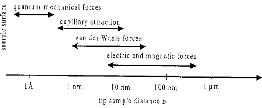
Different other forces also act on the tip. With increasing distance these forces have a different decay rate which is indicated in the figure 2 (18).

Figure 2: action of attractive and repulsive forces and their working distances.

Electrostatic forces

Above 10 nm distance between tip and sample surface next to the magnetic forces also electrostatic forces are the most important influence on the tip. The electrostatic force is given by:

2 el ts

C

F

V

z







38

Where C is the electrical capacity between tip and sample and V_ts is the applied voltage. For a conductive tip this force is always attractive, even if both tip and sample have the same voltage. In the case of an insulating sample, electric surface charges can act on the tip by Coulomb forces. On insulator, due to the scanning motion even charging can occur. Usually these two effects are not important for magnetic media, since the materials are conductive enough. In constant signal mode operation often a voltage is applied between tip and sample to keep the overall force (force derivative) positive so that a regulation loop can keep it constant. This technique is called biasing (18).

Van der Waals Force

Below 10 nm tip-sample distance the influence of the Van der Waal force increases. This type of force originates from the induced electromagnetic dipole-dipole interaction between atoms. In general between two atoms a decay of r7 can be assumed for this force. The magnetic dipolar interaction instead decays as r3. For this reason when the tip is very close to the sample surface, the Van Der Walls forces are very strong, but when the tip is lifted the Van Der Walls forces rapidly decrease while the dipolar interaction remains strong. This is the principle on which the MFM works: in the first pass the tip is kept close to the surface and it feels the Van der Walls forces and in this way it traces the topography. Knowing the topography it is possible to pass a second time with a fixed lift height at which the Van der Walls forces are neglectable but magnetic forces are still strong and in this way only the magnetic forces are accounted for.

Capillary Forces

If measurements are performed in ambient conditions capillary forces need to be accounted for if the radius of the contact is less than the Kelvin radius. Below this dimension vapors (usually water) condense into the contact area. The Kelvin radius is given by

39

log(

)

V

r

RT

p p





where  is the surface tension, R is the universal gas constant, T is the temperature, V is the molar volume and ps is the saturation vapor pressure. Due to the large tip-sample separations capillary

forces are assumed to be negligible in this study.

The Multimode SPM – Nanoscope IIIa

The instrument in our laboratory is a Digital Instruments Nanoscope IIIa. The image of the head of the microscope is reported below in figure 3 (17).

Figure 3: representation of the “head” of the MFM

Images consist of raster-scanned, electronic renderings of sample surfaces. There are three default sizes: 128 x 128 pixels, 256 x 256 pixels, and 512 x 512 pixels. In addition, nine width-to-height aspect ratios may be specified by the user: 1:1, 2:1, 4:1, 8:1, 16:1, 32:1, 64:1, 128:1 and 256:1.

40

Thus, it is possible to obtain “strip scans” which require less time to capture. One can scan up to 200μm laterally (in X and Y) and 10μm vertically (Z axis).

The MultiMode is so called because it offers multiple SPM modes, including AFM, ECAFM, ECSTM, STM and TappingMode. With this instrument it is possibile to perform AFM measurements of the topography following different method:

Contact AFM—Measures topography by sliding the probe tip across the sample surface. Operates in both air and fluids

TappingMode AFM— Measures topography by tapping the surface with an oscillating tip. This eliminates shear forces which can damage soft samples and reduce image resolution. This is now the technique of choice for most AFM work.

Phase Imaging—Provides image contrast caused by differences in surface adhesion and viscoelasticity.

Non-contact AFM—Measures topography by sensing Van der Waals attractive forces between the surface and the probe tip held above the surface. It provides lower resolution than either contact AFM or TappingMode.

Interleave MODE is a feature of NanoScope software which allows the simultaneous acquisition of two data types. After each main scan line trace and retrace (in which topography is typically measured), a second (Interleave) trace and retrace is made with data acquired to produce an image concurrently with the main scan. Typical applications of interleave scanning include MFM (magnetic force microscopy). During the interleave scan, the feedback is turned off and the tip is lifted to a user selected height above the surface to perform far field measurements such as MFM. The lift mode measures MFM or other long range interaction in the second pass, while in the first pass the topography is measured in tapping mode at a smaller distance at which Van der Waals forces prevail figure 4 (17).

41

Figure 4: scheme of the lift operation mode; in the first pass the microscope traces the topography; the second pass is performed at a fixed distance (lift distance) at which long range forces (like magnetic coupling interaction) prevail.

The four elements of the quad photodiode (position sensitive detector) are combined to provide different information depending on the operating mode. In all modes the four elements combine to form the SUM signal. The amplified differential signal between the top two elements and the two bottom elements provides a measure of the deflection of the cantilever. This differential signal is used directly in the contact AFM. It is fed into an RMS converter (or phase module if attached) for TappingMode operation.

Figure 5 (17) shows the arrangement of the photodiode elements in the MultiMode head. Different segments of the photodetector are used for generating AFM and LFM (lateral force microscope) signals.

42

Figure 5: the four elements photodiode for the analysis of the reflected beam, the interpretation of the detected signal is performed by the software.

A version of the TappingMode tip is the MFM probe. This is basically a crystal silicon TappingMode probe having a magnetic coating on the tip. As the magnetized tip oscillates through magnetic fields on the sample surface, it modulates the cantilever’s phase and frequency. These are monitored, providing a measure of magnetic field strength and providing images of magnetic domains.

AC voltages applied to the scanner crystal X-Y axes produce a raster-type scan motion as represented in Figure 6.

43

Figure 6: the x-y scanner is moved by piezo-element actuators.

Magneto-Optical Kerr Effect

The magneto-optical Kerr effect (MOKE) is a technique employed to investigate the magnetization mechanisms of some sample discussed in this work. Therefore it is helpful to describe the physical basics and the measurements setup of this technique.

Introductory arguments

In the magneto-optical Kerr effect (MOKE) (19) the interaction between a polarized light and magnetization of a ferromagnetic sample causes the change of polarization and/or intensity of the light beam reflected by the sample surface. The transmission analogous to the Kerr effect is the Faraday effect, where the polarization of the light beam transmitted through the ferromagnetic material is changed from the polarization of the incident light beam (20). The Kerr effect can be

44

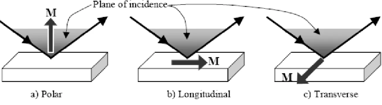
observed in three different dispositions of the magnetization with respect to both the plane of incidence of the light and the sample reflecting surface (21) (figure 7).

Figure 7: Polar, Longitudinal and Transverse configuration depending on the orientation of the incidence plane with respect to the magnetization vector.

In the polar configuration the magnetization is perpendicular to the sample surface and it is performed at normal incidence. Longitudinal and transverse MOKE operate at a certain angle of incidence, with a magnetization parallel to the sample surface, either parallel (longitudinal) or perpendicular (transverse) to the optical plane of incidence. The simplest model to explain the MOKE phenomenon is to consider a Lorentz-Drude theory for a metallic film. The incident light causes an electrons oscillation parallel to the plane of polarization. In the presence of a non-ferromagnetic sample, the polarization plane of the reflected light is the same as the incident light. When the sample has a magnetization that acts on the oscillating electrons through a Lorentz force, like an internal magnetic field, the result is a second oscillating component perpendicular to the direction of the magnetization and to the primary motion. Using a linearly polarized incident light, the polar and longitudinal MOKE yield the orthogonally polarized component upon reflection whereas the transverse geometry only affects the intensity, i.e. the amplitude of the incident polarization (22). However, the complexity of MOKE theory requires a quantum description, that stems from the need for explaining the large magneto-optical effect in the ferromagnetic

45

materials (23). The explanation could be found in the spin-orbit coupling, introduced by Hulme (24) and improved by Kittel (25) and Argyres (26). The spin-orbit interaction couples the magnetic moment of the electron with its motion, connecting the magnetic and optical properties of a ferromagnet. This effect is present also in the non-magnetic materials, but it is only in the ferromagnets that it manifests itself thanks to the unbalanced number of spin up and spin down electrons.

Mathematic formalism

The formalism to explain the MOKE effect is the same used for the other magneto-optical effects. If we consider a linearly polarized light as a superposition of right and left circularly polarized light, we see how, without an external magnetic field, a left-circularly polarized light will drive the electrons into left circular motion and a right-circularly polarized light will drive the electrons into right circular motion. The radius of the electron orbit for left and right circular motion will be the same and, since the electric dipole moment is proportional to the radius of the circular orbit, there will be no difference between the dielectric constants for both circularly polarized electromagnetic waves.

An interesting effect occurs when dealing with a ferromagnetic sample because a net Lorentz force acts on the electrons due to the magnetization of the sample. The Lorentz force introduces an additional small oscillating component to the motion of the electrons in the perpendicular direction both to the magnetization and to the displacement of the electrons. By superimposing the contributions, with their relative phases, the reflected light will result in an elliptical polarization state (27).

Considering the polar Kerr effect at normal incidence, the complex refraction index of the sample is n for the right circularly polarized light and n for the left circularly polarized light, where n