On seismic design and advanced numerical modelling of flexible cantilever walls under earthquake loading including cyclic mobility

(1)

Doctoral Thesys in Geotechnical Engineering , G. Li Destri Nicosia

On seismic design and advanced numerical

modelling of flexible cantilever walls under

earthquake loading including cyclic mobility

By

Giovanni Li Destri Nicosia

Dottorato di Ricerca in Ingegneria Geotecnica Ciclo XXII

Coordinator: Prof. Michele Maugeri

Supervisor: Prof. Michele Maugeri

(2)

(3)

ABSTRACT

Pseudostatic design methods for seismic design of retaining structures are very widely spread in aseismic design codes worldwide. These methods are based on a crude simplification of reality, nevertheless observational evidence of earth retaining structures designed using simplified methods based on limit equilibrium show their good overall performance except for some situations where saturated granular backfill is present. The aim of this work is first to critically describe the main tools available today for the analysis and seismic design of flexible retaining structures. Secondly to apply different methodology to a practical benchmark study case describing all issues related to the correct application of simplified methodologies and issues regarding the sophisticated numerical approaches. Finally results obtained by the simplified and the sophisticated approaches are evaluated and compared Differences, advantages and disadvantages between the simplified and the more sophisticated approaches are illustrated along with those between the numerical analysis themselves. Analyses are performed for the case of dry and saturated backfill for both simplified and numerical approach and the effectiveness of the simplified method comparing to numerical analyses is assessed in both cases.

A good agreement between Finite Elements (DYNAFLOW) and Finite Difference (FLAC) approach was reached for the case of dry backfill and a special numerical application of the pseudodynamic approach is also presented. For its relatively simple implementation and the fairly good agreement with more sophisticated analysis shown for the benchmark case configuration considered, such procedure appears to be an effective tool and good alternative to classical pseudostatic approach for the seismic design/assesments of retaining structures in earthquake prone regions. Time history analyses on the other hand are time consuming require a more experienced user and the additional task to selected a representative set of spectrum compatible accelegrams.

The case study of saturated backfill included in the present work presents a simplified methodology to assess liquefaction potential and the comparison with more sophisticated analyses (OPENSEES and FLAC) allows some considerations on the limits and strength of such methodology.

(4)

(5)

ACKNOWLEDGEMENTS

I would like to thank all those who gave me support for carrying out this Thesis including Professor Maugeri from the University of Catania, Eric Parker from D’Appolonia SpA, Professor A. Elgamal from UCSD for his support on Opensees PDMY model, Prof A Pecker and Prof J H Prevost for their support on Dynaflow, Dr Carlo Lai from Eucentre and Dr John Perry from Mott MacDonald LtD.

(6)

LIST OF FIGURES

Page

Figure 2.1 Cross section of Konakano No. 1 Quaywall in Port of Hachinoe [Kawakami and Asada, 1966] ...4 Figure 2.2 Damage to Konakano No. 1 sheetpile quaywall in Port of Hachinoe [Hayashi and

Katayama, 1970] ...5 Figure 2.3 Cross section of Konakano No. 1 Quaywall in Port of Hachinoe [Hayashi and

Katayama, 1970] ...5 Figure 2.4 Cross section of Konakano No. 1 Quaywall in Port of Hachinoe [Hayashi and

Katayama, 1970] ...6 Figure 2.5 Cross section of a quay wall at Ohama No.2 Wharf [Iai and Kameoka, 1993] ...7 Figure 2.6 Damage at Ohama No. 2 Wharf [Iai and Kameoka, 1993] ...7 Figure 2.7 Deformation along the face line at Ohama No. 2 Wharf (a) Cross section, (b)

Distribution along the face line [Iai and Kameoka, 1993] ...8 Figure 2.8 Cross section of Konakano No. 1 Quaywall in Port of Hachinoe [Hayashi and

Katayama, 1970] ...9 Figure 2.10 Higashinada Wastewater Plant Site Plan ...11 Figure 2.11 Retaining wall along the Inlet between the Island and the mainland moved toward

the water (north) 2 to 3 m ...11 Figure 2.12 Accelerograms recordings at Adapazari station (SKR) and calculated velocity and

displacement time histories. ...12 Figure 2.13 MSE bridge approach (a) plan view of approach fill with damage concentration;

(10)

Figure 2.14 Damage detail for (a) E1 and (b) E2 on eastern MSEW face (phots after Ozbakir)

...14

Figure 2.15 Damage of retaining wall along National Highway Route 17 ...15

Figure 2.16 Reconstruction of damaged retaining wall along National Highway Route 17 ....15

Figure 3.1 Relative soil wall displacements for rest a), active b) –passive c) states [Das B.M. , 2007] ...18

Figure 3.2 Movement of "soil" surrounding model retaining wall [Lambe, T.W., Whitman, V. W, 1979] ...19

Figure 3.3 Stress paths from at rest conditions to active or passive state [Lambe, T.W., Whitman, V. W, 1979] ...19

Figure 3.4 (a) At rest conditions (b,c) Rankine’s states of plastic equilibrium illustrating active conditions (d) Mohr stress and strength diagrams (e,f illustrating passive conditions) [Prakash, S., 1981] ...20

Figure 3. 5 Strains required to reach passive and active state in dense sand [Lambe, T.W., Whitman, V. W, 1979] ...21

Figure 3.6 Nature of variation of lateral earth pressure [Das B.M. , 2007] ...22

Figure 3.7 Coulomb's active pressure [Das B.M. , 2007] ...22

Figure 3.8 Coulomb’s passive pressure [Das B.M. , 2007] ...23

Figure 3.9 Nature of failure surface in soil with wall friction (a) active pressure (b) passive pressure [Das, 2007] ...24

Figure 3.10 Active earth pressure under earthquake load (a) force on failure wedge (b) forces polygon [Prakash, S., 1981] ...25

Figure 3.11 (a) Static horizontal earth pressure (b) Dynamic horizontal earth pressure (Sherif and Fang [1983]). ...27

Figure 3.12 Point of application of incremental dynamic active thrust versus horizontal acceleration coefficient [Ishibashi and Fang, 1987]. ...28

Figure 3.13 Static and Dynamic earth pressure distribution behind 1-m high flexible wall test no. 4 [Nandkumaran, 1973] ...30

Figure 3.14 Peak ground or table velocity versus dynamic increment of earth pressure for flexible and rigid wall [Prakash and Nandkumaran, 1979] ...30 Figure 3.15 Limiting values for horizontal acceleration kh*·g [Ebeling and Morrison, 1992] .32

(11)

Figure 3.16 Force acting on a wall retaining c-φ soil and subjected to an earthquake type load

[Prakash, 1968] ...34

Figure 3.17 (Nac)stat versus φ for all n [Prakash, 1968] ...34

Figure 3.18 (Naq)stat versus φ for n=0 [Prakash, 1968] ...35

Figure 3.19 (Naq)stat versus φ for n=0.2 [Prakash, 1968] ...35

Figure 3.20 (Naγ)stat versus φ for n=0 [Prakash, 1968] ...36

Figure 3.21 (Naγ)stat versus φ for n=0.2 [Prakash, 1968] ...36

Figure 3.22 λ versus φ [Prakash, 1968] ...37

Figure 3. 23 Composite failure surface and forces considered ...39

Figure 3. 24 Initial and transformed geometry [Lancellotta, 2007] ...41

Figure 3. 25 Stress discontinuity analysis: a) fan of stress discontinuities; b) Mohr circles relative to zone 1 and zone 2; c) Mohr circle relative to conventional passive zone [Lancellotta, 2007] ...42

Figure 3.26 Comparison of coefficient of passive resistance [Lancellotta, 2007] ...43

Figure 3. 27 Anchored bulkheads extending below water level [Towhata and Islam, 1987] ...45

Figure 3. 28 Soil wedge and acting forces/pressures [Towhata and Islam, 1987] ...45

Figure 3. 29 Model for dynamic pressure increment [Richard et al, 1999]...47

Figure 3. 30 Response of Soil-Wall system by Superposition [Richard et al, 1999] ...47

Figure 3.31 Seismic free field (Richard and Shi [1994]) ...49

Figure 3.32 Shear stress effect due to s and kh (Richard and Shi [1994]) ...50

Figure 3. 33 Soil wall system investigated: a) Base-excited system b) Force-excited system [Veletsos and Younan, 1997] ...51

Figure 3.34 Distributions of wall pressure for statically excited systems with different wall and base flexibilities (v = 1/3, µw= 0):(a)for dӨ= 0;(b)for dw=0) [Veletsos and Younan, 1997, 2000] ...54

Figure 3.35 Normalised effective heights for statically excited systems with different wall and base flexibilities (v = 1/3, µw= 0) [Veletsos and Younan, 1997] ...55

Figure 3.36 Amplification Factors for Base Shear in Wall of Harmonically Excited Systems with Different Wall and Base flexibilities (v = 1/3,δ = 0.1,µw=0, and δw = 0.04): (a)for dӨ = 0; (b)for dw = 0 [Veletsos and Younan, 1997] ...56

(12)

Figure 3. 37 Maximum Amplification Factors for Base Shear and Top Displacement Relative to Base of Harmonically Excited Systems with Different Wall and Base Flexibilities (v = 1/3,δ = 0.1, µw = 0, and δw = 0.04): (a) Base Shear; (b) Top Relative Displacement

[Veletsos and Younan, 1997] ...56 Figure 3. 38 Amplification Factors for Base Shea in Wall of Systems with Diferent Wall and

Base Flexibilities Subjected to El Centro Earthquake Record (v = 1/3,δ = 0.1, µω. = 0,

and δw=0.04): (a) for dӨ = 0; (b) for dw, = 0 [Veletsos and Younan, 1997] ...57

Figure 3. 39 Normalized Values of Maximum Base Shear In Wail of Syst.ms with Different Wail and Base Flexibilities Subjected to El Centro Earthquake Record (v = 113, 8 = 0.1, p.,,. = 0, and 5,, = 0.04): (a) for d, = 0; (b) for d.,. = 0 [Veletsos and Younan, 1997] ...57 Figure 3. 40 The finite-element discretization of the examined single-layer systems. The base

of the model is fixed, while absorbing boundaries have been placed on the right-hand artificial boundary [Psarropoulos et al, 2005] ...59 Figure 3. 41 Comparison between the normalized values of base shear (∆PE)St and overturning

moment (∆ME)St from the analytical formulation (continuous line) of Veletsos and

Younan [1997] and those of the numerical simulation (dots). Quasi-statically excited systems with different wall and base flexibilities (dw and dӨ) [Psarropoulos et al, 2005].

...59 Figure 3. 42 Effect of soil inhomogeneity on the elastic dynamic earth-pressure distribution

for a rigid fixed-base wall (dwZ0, dqZ0) and for a flexible fixed-base wall (dwZ40, dqZ0). Comparison with the corresponding curves for the homogeneous soil from Fig. 4 [Psarropoulos et al, 2005]. ...60 Figure 3. 43. Distribution of the wall pressures in the case of resonance (ω=ω1): (a) dӨ=0.5 (b)

dӨ=5 [Psarropoulos et al, 2005] ...61

Figure 3. 44 Maximum dynamic amplification factors AQ and AM for the resultant

overturning moment, respectively, in the case of resonance (ω=ω1) [Psarropoulos et al,

2005] ...61 Figure 3. 45 Schematic diagram showing the FE discretization zones [Madabhushi and Zeng,

2007] ...62 Figure 3.46 Variation of bending moment at 80g in a) saturated case and b) dry case

(13)

Figure 3.47 Bending moment distribution along the wall for the saturated (a) and unsaturated (b) case during three earthquakes [Madabhushi and Zeng, 2007] ...63 Figure 3. 48 Profile of the centrifuge model XZ3 for (EQ3) at 0.3g PGA before and after

earthquake [Madabhushi and Zeng, 2007]. ...64 Figure 4.1 The main stages of computer-based simulation: idealization, discretization and

solution [notes from Advanced Finite Element course of Prof. Carlos Felippa at

University of Colorado Boulder] ...68 Figure 4. 2 2D continuum elements [DYNAFLOW user manual, 2006] ...70 Figure 4. 3 Basic explicit calculation cycle [FLAC 5.0 user manual, 2005] ...72 Figure 4. 4: Basic framework of OpenSees (OpenSees and NEESgrid Component User

Workshop, 2008)...75 Figure 4.5: Construction of the model builder object and definition of materials in Open Sees.

...76 Figure 4.6: Construction of the finite element mesh...76 Figure 4.7: Definition of loading pattern. ...77 Figure 4. 8: Construction of the recorded objects to save nodel displacements and

accelerations and element stress, strain and pressure data with each time step. ...77 Figure 4. 9 Construction of analysis objects and execution of analysis. ...78 Figure 4. 10 Soil liquefaction and tilting during Niigata earthquake 1964

[http://www.ce.washington.edu/~liquefaction/html/quakes/niigata/niigata.html] ...79 Figure 4.12 Simple shear idealization of soil under earthquake loading ...80 Figure 4.13 Strain level and types of soil mechanical behaviour in simple cyclic shear

[Silvestri, 2005]...82 Figure 4.14 Curve stress-cyclic strain [Pecker, 1984] ...83 Figure 4. 15 Model parameters for Hardin-Drevnich method [Pecker, 1984] ...83 Figure 4.16 Modulus reduction curves for fine-grained soils of different plasticity (Vucetic

and Dobry[1991])...83 Figure 4. 17 Collapsed bridge after 1964 Niigata Earthquake (University of Washington Web Site). ...84 Figure 4. 18 Iwan model [1967] ...86 Figure 4. 19 Schematis representation of two hardening types [Elgamal et al, 2003] ...87

(14)

Figure 4. 20 Mohr Coulomb and Tresca Yield surfaces in principal stress space [FLAC 5.0 user manual, 2005] ...88 Figure 4.21 Comparison between Coulomb-Matsuoka criteria on deviatoric plane

[Matsuoka,1985] ...91 Figure 4.22 Stress–strain relationship and stress path for undrained cyclic triaxial test on

reclaimed gravely Masado soil (Hatanaka et al., 1997), which developed major

liquefaction-induced deformations during the 1995 Kobe, Japan earthquake. ...93 Figure 4.23 Schematic of constitutive model response showing shear stress, effective

confinement, and shear strain relationship [Elgamal et al., 2003]. ...94 Figure 4.24 Conical yield surface in principal stress space and deviatoric plane [after Prevost, 1985; Parra, 1996; Yang, 2000]. ...95 Figure 4.25 Dilation function performance for a given γy and different user defined rates of

dilation [Elgamal et al., 2003]. ...97 Figure 4. 26 Dilation function performance for a given γy and different user defined rates of

dilation [Elgamal et al., 2003]. ...98 Figure 4. 27 Schematic of constitutive model response showing (a) octahedral stress τ,

effective confinement p’ response, (b) octahedral stress τ, octahedral strain γ response, and (c) configuration of yield domain [Elgamal et al., 2003]. ...99 Figure 4. 28 Initial yield domain at low levels of effective confinement [Elgamal et al., 2003]. ...100 Figure 4. 29 Mroz(1967) deviatoric hardening rule ...101 Figure 4. 30 New deviatoric hardening rule (after Parra, 1996). ...102 Figure 4.31 Model for seismic analysis of surface structures and free field mesh [FLAC 5.0,

User manual] ...105 Figure 4.32 An interface represented by sides a and b, connected by shear (ks) and normal (kn)

stiffness spring [FLAC5.0, User manual] ...107 Figure 4.33 Slide line [DYNAFLOW user manual, 2006] ...108 Figure 5.1 Anchored sheet piles in London Clay (telephone switch centre) [M. Puller, 1996].

...111 Figure 5.2 Diaphragm wall anchored below existing property and highway (Croydon, UK)

(15)

Figure 5.3 Precast diaphragm wall using Prefasil system (Schipol, Nederlands) [M. Puller,

1996]. ...112

Figure 5.4 Composite use of contiguous bored pile walls and steel soldier beams (Courtesy of Bauer, Stuttgart) [M. Puller, 1996]. ...113

Figure 5.5 Benchmark model geometry...115

Figure 5. 6 Comparison between experimental [Palmieri, 1995] and analytical [Ishibashi and Zhang, 1993] degradation curve ...117

Figure 5.7 Lateral pressure distribution for fixed earth support [CIRIA,1995]. ...117

Figure 5.8 Lateral pressure distribution for fixed earth support, seismic case[CIRIA,1995]. 118 Figure 5. 9 Bending moment distribution for pseudostatic method (Soil D and different PGA equal to 0.35g, 0.25g and 0.15g respectively for zones 1,2 and 3). ...119

Figure 5.10 Lateral pressure distribution for fixed earth support, seismic case with saturated backfill and pore pressure build up [Ebeling and Morrison, 1992]. ...121

Figure 5.11 Bending moment distribution for pseudostatic method and saturated case (Soil C and different PGA equal to 0.25g and 0.15g respectively zones 2 and 3). ...121

Figure 6. 1 (Up) UHS on stiffsoil for different return periods [Menon et al., 2004] (Down) deagregation for 475 years [Menon et al., 2004] ...124

Figure 6. 3 Erzincan accelerogram (scaled 0,15g) ...127

Figure 6. 4 Tortona accelerogram (scaled 0,15g) ...127

Figure 6. 5 Pseudo acceleration elastic spectra (5% damping) for input accelerograms compared to EC8 Type1 spectrum ...128

Figure 6.6 Pseudo velocity elastic spectra (5% damping) for input accelerograms compared to EC8 Type1 spectrum...128

Figure 7. 1 FLAC model for benchmark case...130

Figure 7. 2 Bending moment versus depth during excavation phases ...131

Figure 7. 3 Displacement versus depth during excavation phase ...132

Figure 7.4 Bending moment from FLAC pseudostatic and fixed earth support scheme ...133

Figure 7.5 DYNAFLOW model ...134

Figure 7. 6 Bending moments from DYNAFLOW model during excavation phases ...134

Figure 7. 7 Displacements from DYNAFLOW model during excavation phases ...135

Figure 7. 8 Bending moments from DYNAFLOW (dyn) and FLAC (flac) models during excavation phases...136

(16)

Figure 7. 9 Displacements from DYNAFLOW (dyn) and FLAC (flac) during excavation (exc.) phases. ...136 Figure 7. 10 Pseudostatic loading for Kh=0.0937 ...136 Figure 7. 11 Displacement time histories for points placed at the bottom (224) and mid height (223) of the backfill. ...138 Figure 7. 12 Displacement spectra using as input displacement time histories for points placed

at the bottom (224) and mid height (223) of the backfill. ...138 Figure 7. 13 Bending moments for Chalfant Valley 0.15g (left wall a) and right wall b)) and

Erzincan 0.15g (left wall c) and right wall d)) ...140 Figure 7. 14 Bending moments for Tortona 0.15g (left wall a) and right wall b)) ...141 Figure 7. 15 Average of bending moments from all accelerograms (left wall a) and right wall

b)) ...141 Figure 7. 16 Minimun, residual and maximm displacements for left-right walls for Chalfant

Valley, Erzincan scaled 0.15g ...143 Figure 7. 17 Minimun, residual and maximum displacements for left- right walls for Tortona

0.15g...144 Figure 7. 18 Average of results from three accelerograms for minimun, residual and maximm displacements for left- right walls 0.1...144 Figure 7.19 Maximum acceleration along the wall for Cahlfany Valley a), Erzincan b)

Tortona c) input motion scaled 0.15g PGA and average ...145 Figure 7. 20 Displacements (maximum, minimum and residual) and bending moments for

both walls, for Tortona, Erzincan and Chalfant scaled 0,15g FLAC. ...148 Figure 7. 21 Horizontal pressure distribution for both walls, for Tortona, Erzincan and

Chalfant scaled 0,15g FLAC...149 Figure 7. 22 Disp. profiles (maximum, minimum and residual) and bending moments for

both walls, for Tortona, Erzincan and Chalfant scaled 0,35g FLAC. ...150 Figure 7. 23 Horizontal pressure distribution for both walls, for Tortona, Erzincan and

Chalfant scaled 0,35g FLAC...151 Figure 7. 24 Disp. profiles (maximum, minimum and residual) and bending moments for both walls, for Tortona, Erzincan and Chalfant scaled 0,6g. FLAC ...152 Figure 7. 25 Horizontal pressure distribution for both walls, for Tortona, Erzincan and

(17)

Figure 7. 26 Ratio between peak bending moments of left and right wall for several PGA and input motions. ...154 Figure 7. 27 Ratio between peak top wall displacement of left and right wall for several PGA

and input motions. ...154 Figure 7. 28 Shear modulus degradation curves for FLAC model versus Ishibashi and Zhang

FLAC ...156 Figure 7. 29 Variation of hysteretic damping for FLAC model versus Ishibashi and Zhang

FLAC ...157 Figure 7. 30 Static and maximum dynamic pressures and bending moments along left and

right wall for Tortona 0.15g seismic input FLAC. ...158 Figure 7. 31 Static and maximum dynamic pressures and bending moments along left and

right wall for Tortona 0.35g seismic input FLAC. ...159 Figure 7. 32 Static and maximum dynamic pressures and bending moments along left and

right wall for Tortona 0.6g seismic input FLAC ...160 Figure 7. 33 Ratio between peak bending moments of left and right wall for Tortona event

scaled at several PGA and elastic perfectly plastic (MC) or fully non linear (Hyst.) model...161 Figure 7. 34 Displacement profiles (maximum, minimum and residual) for left and right wall

for Tortona 0.15g (upper) and Tortona 0.35g (lower) FLAC. ...162 Figure 7. 35 Displacement profiles (maximum, ,minimum and residual) for left and right wall for Tortona FLAC. ...163 Figure 8.1 Relationship of void ratio to relative density used for PDMY material (values

recommended by Opensees and calculated by the formula in Table 8.2). ...168 Figure 8.2 Relationship of soil mass density to the relative density used for the PDMY

material (values recommended by Opensees and calculated by the formula in Table 8.2). ...168 Figure 8.3 Relationship of reference shear modulus to relative density used for the PDMY

material (values recommended by Opensees and calculated by the formula in Table 8.2). ...169 Figure 8.4 Relationship of reference bulk modulus to relative density used for the PDMY

material (values recommended by Opensees and calculated by the formula in Table 8.2). ...169

(18)

Figure 8.5 Relationship of friction angle to relative density used to define the PDMY material material (values recommended by Opensees and calculated by the formula in Table 8.2). ...170 Figure 8.6 Relationship of phase transformation angle to relative density used to define the

PDMY material (values recommended by Opensees and calculated by the formula in Table 8.2). ...170 Figure 8. 7 Dilation parameters. (a) First dilation parameters comparion between

reccommended values by Opensees and linear interpolation function (b) Second dilation parameter comparison bewteen reccommended values by Opensees and linear

interpolation function. ...172 Figure 8. 8 Liquefaction parameters. Relationships between liquefaction parameters and

relative density used to define PDMY material. Recommended values are represented by diamonds and Equations 8.9 to 8.13 are represented by lines. ...173 Figure 8. 10 Input cyclic force applied to top element under an effective confining pressure of 3.5 kPa...175 Figure 8. 11 Modulus reduction and damping curves for trial with automatic modulus

reduction curve generation. The solid line represents the automatically-generated curve, crosses represent Darendeli’s curve, and circles represent actual model behaviour. ...175 Figure 8. 12 Results of a model execution with 0.23 CSR and 45% Dr; (a) displacement at

element top (b) excess pore pressure ratio increase with time and (c) shear stress versus strain and deviatoric versus effective confining stress. ...176 Figure 8. 13 Results of a model execution with 0.23 CSR and 75% Dr; (a) displacement at

element top (b) excess pore pressure ratio increase with time and (c) shear stress versus strain and deviatoric versus effective confining stress. ...177 Figure 8. 14 SPT clean-sand base curve for magnitude 7.5 earthquake with data from

liquefaction case histories (modified from Seed et al., 1985) (Youd et al., 2001) ...179 Figure 8. 15 Recommended magnitude scaling factors for earthquakes of varying magnitude. Values from the centre of the hatched area were used for this analysis (Youd et al., 2001) ...180 Figure 8. 16 Number of equivalent uniform stress cycles for earthquakes of different

(19)

Figure 8. 17 Comparison between predicted relationship NL/Dr and calculated by OPENSEES

element test calibration process. ...181 Figure 8. 18 FLAC geometry and grid for the shaking table test simulation. ...182 Figure 8. 19 Comparison between Opensees, FLAC and reference curves for number of cycles

to liquefaction (NL) and cyclis stress ration (CSR) for different values of relative density

(Dr%). ...183 Figure 8. 20 Reduction factor to estimate the variation of cyclic shear stress depth below level or gently sloping ground surfaces (Kramer, 1996). ...185 Figure 8. 21 Idealized soil profile used for comparison among analysis methods. ...186 Figure 8. 22 FLAC model grid for the saturated case study. ...191 Figure 8. 23 Relative increments in displacement and bending moments for dry and saturated

cases. ...192 Figure 8. 24 Comparison between pore pressure ratio ru prediction using CSR method and

FLAC for Tortona earthquake scaled to PGA equal 0.15g a) and 0.25g b). ...193 b) Figure 8. 25 Maximum bending moments along left and right wall for Tortona 0.15g PGA

a) and 0.25g PGA b) from FLAC and pseudostatic analyses. ...194 b) Figure 8. 26 Maximum wall displacements along left and right wall for Tortona 0.15g PGA

(20)

LIST OF TABLES

Page

Table 3.1 Particulars of test data on 1-m flexible wall [Nandkumaran, 1973] ...29

Table 3.2 Particular of test data on 1-m high rigid wall [Nandkumaran, 1973] ...29

Table 3.3 Computation of seismic earth pressure by various methods ...40

Table 3.4 Basic solution requirements satisfied (S) or not satisfied (NS) by the various methods of analysis [Pott and Zdravkovic, 1999] ...66

Table 4. 1 Constitutive input parameters for model Elgamal 2003 ...103

Table 4. 2 Main differences between FEM and FDM approach...109

Table 4. 3 Main differences between DYNAFLOW, Opensees and FLAC ...110

Table 5. 1 Mechanical properties for unit length of diaphragm wall ...114

Table 5. 2 Soil properties ...114

Table 5. 3 Calculated embedment depth and total wall height ...119

Table 5. 4 Calculated embedment depth and total wall height. ...122

Table 6. 1 Example of deaggregation analysis results ...125

Table 6. 2 Main features of seismic events considered [PEER, ISESD] ...126

Table 7. 1 Peak values for bending moments and top wall displacements for different PGA and input motions. ...146

Table 7. 2 Peak values for bending moments and top wall displacements for different PGA and material models ...161

Table 8.1 Geotechnical and constitutive reference parameters (http://cyclic.ucsd.edu/opensees) ...166

(21)

Table 8.3 Constitutive parameters ...171 Table 8. 4 Model constants ...174 Table 8.5 Results summary for Opensees element test...178 Table 8. 6 Estimated cyclic shear stresses, factor of safety, and excess pore pressure ratio with

depth based on cyclic stress approach for a loose sand layer densities of (N1)60 = 10 for Tortona accelerogram scaled at a) 0.15g PGA, b) 0.25g PGA. ...187

(22)

1 INTRODUCTION.

Earthquake resistant design of earth retaining structures like retaining walls is an important issue to reduce the devastating effect of earthquake hazard. The seismic behaviour of retaining structures under seismic conditions is a complex soil structure interaction phenomenon even if the case of gravitational loading alone is considered. The case of earthquake loading is even more complex to address.

Despite such complexity, due to the widespread presence of retaining type of structures many studies and investigations are among the first in geotechnical engineering and as a result there are several categories of design/analysis methodologies available for both static and seismic design of flexible retaining structures which are briefly described in the following. A correct and efficient use of each methodology requires an understanding of the underlying hypothesys.

For engineering design reference codes such as European EC8, the new Italian seismic code (Allegato 4, OPCM No. 3274 e 3316) or Italian Building Code (D.M. 14/01/2008) for routine day to day design of retaining walls, advocate the use of simplified design methodologies based on limit equilibrium and pseudostatic methods. The application of these simplified methodologies requires an understanding of the possible failure mechanisms and the most convenient yet safe approach to evaluate the limit loads.

An alternative approach for seismic design/assessment of retaining structures is that based on numerical methods and a variety of methodologies are available. In this respect it is important to illustrate which are advantages and limitations of each type of method. Even if an in depth descriptions of numerical analysis is not the purpose of this work, to illustrate advantegs and limitations of different methodologies, it is of interest to have a picture of the main framework in which Finite Elements and Finite Difference methods can be placed. Three numerical codes are used in this work two based on Finite Elements Method (DYNAFLOW and Opensees) and one based of Finite Differences Method (FLAC). The theory beyond these numerical tools is very vast and their correct engineering application requires a clear idea on the main limits beyond the modelling and the solution process. For this reason a wide range of topics such as non linear cyclic soil behaviour or plane wave propagation theory, non linear iterative solution strategies and probabilistic hazard assessment for seismi input selection must be correctly understood.

(23)

Following an empirical approach, the methodology of this work is based on the choice of a design benchmark reference problem, on the application of pseudostatic and more refined numerical tools and finally on the analysis of the results obtained using different methodologies. The conclusions of this application are intended to give some guidance for choosing the most convenient method for assessment and design of flexible retaining structures under earthquake loading and for understanding the reasons of the limitations of the results obtained. Since performance of flexible retaining structure under earthquake loading has been poor [Gazetas et al, 2004] for the case of saturated backfill, both cases of saturated and unsaturated backfill are considered.

The work is structured in the following way: in the next Chapter a review of case histories of documented failures of earth retaining structures is outlined, in Chapter 3 a review of available methods for earth retaining structures seismic analysis/design is presented, Chapter 4 contains a description of a wide range of general modelling issues for geotechnical earthquake engineering, in Chapter 5 the model analysed is described and the pseudostatic code based design approach applied. In Chapter 6 the methodology for the selection of the accelerograms and the input accelerograms is introduced. In Chapter 7 and Chapter 8 a description of the numerical models used for the analyses is done and the results of the numerical analysis are presented respectively for the dry and saturated cases. Chapter 9 contains the conclusions.

(24)

2 CASE HISTORIES AND MOTIVATION.

Field observation and reporting of damage caused by earthquake allows engineers to learn about limitations of design practice and to identify most critical failure mechanisms and the causes behind them. Several examples of failures of retaining structures under earthquake loading from literature are described in the following sections.

2.1 Damage to earth structures by the Niigata Earthquake 1964.

On June 16, 1964 a great earthquake occurred at Niigata Prefecture, Japan. Soil formation in this area consists chiefly of recent alluvial deposit and recently deposited artificial fill which are composed of relatively uniform, loose and saturated sand. The vibration due to earthquake induced the liquefaction of saturated loose sand and caused much damage to earth structure and foundation.

Structures in harbours and revetments of river banks were also moved, sttled or overturned by the earthquake, since the grounds were liquefied. Almost all structures in Niigata Harbour suffered severely and those of Sakata Harbour were also damaged. Figure 2.1 [Kawakami and Asada, 1966] shows the appearance of damaged Yamashita Wharf in Niigata Harbour, namely the quaywall of steel sheet piles was pushes out 36 cm, the ground behind the concrete anchor plate was subsided and the bed of the sea was heaved up by about 100 cm. This damage was caused by the increase of earth pressure acted on back of sheet piles and the decrease of the resistance of anchor plate of tie rod against sliding, due to liquefaction of sandy backfill.

(25)

Figure 2.1 Cross section of Konakano No. 1 Quaywall in Port of Hachinoe [Kawakami and Asada, 1966]

2.2 Sheet pile walls damage from the Tokachioki Earthquake 1968.

Port and harbour facilities in the southern part of Hokkaido and the northern part of Honshu were damaged by the 1968 Tokachioki earthquake on May 16, 1968 with total sum of damage estimated approximately 5 million U.S. Dollars.

Hayashi and Katayama [Hayashi and Katayama, 1970] include description of damages to several types of port and harbour facilities including caisson breakwaters, gravity types of quay wall and sheetpile bulkhead quay walls with and without batter anchor piles. There were few large-sized mooring facilities which suffered heavy damage and comparatively heavy damage was encountered in lighter’s wharves and sea walls.

Generally speaking, damage to mooring systems and sea walls were similar to those encountered in other previous earthquakes, i.e. swelling of front lines, settlements and cracking of aprons.

• Damage to sheetpile bulkhead:

Typical features of the damage to sheetpile bulkhead were a forward tilting of the wall due to insufficient anchor resistance , development of tension cracks above the anchor in parallel direction to the front line and settlement of backfill surface. In some cases, local breakage of fixation of tie rod to anchor was observed. As an example of heavily damaged sheetpile bulkhead Figure 2.2 shows the largest deformation of Konakano sheetpile bulkhead quay wall. The seaward movement of the front line was about 1 m, a concrete coping of sheetpile was broken with a relative settlement of the apron to the coping was 65 cm.

(26)

Calculated factor of safety for twenty cases of sheetpile shows that for eight of those cases in which factor of safety was less than one for insufficient embedment depth, there was no damage due to bending of sheetpiles or breaking of tie rods showing that current design method for embedment was conservative, but in the bulkheads of such sheetpiles a swelling of front lines ranging from 10 to 30 cm was observed due to the movements of anchor plates.

Figure 2.2 Damage to Konakano No. 1 sheetpile quaywall in Port of Hachinoe [Hayashi and Katayama, 1970]

Records from Niigata earthquake indicate that even for case with safety factor of safety higher than one have sometime shown insufficient anchor resistance and in addition anchoring, is installed in a position most susceptible of soil liquefaction.

(27)

Doctoral Thesys in Geotechnical Engineering , G. Li Destri Nicosia • Damage to sheetpile bulkhead with batter anchor piles:

This type of facilities were more recently introduced hence it had not been subjected to any strong earthquake before. Two facilities of this type were subjected to the earthquake. There was no damage in one case. In the other case of the -5.5m quaywall of Kitahama Pier in Port of Hakodate, however, the fixation point of the sheetpile anchor piles was broken. Cross sections, before and after the earthquake, of the latter structure are shown in Figure 2.4.

Figure 2.4 Cross section of Konakano No. 1 Quaywall in Port of Hachinoe [Hayashi and Katayama, 1970]

2.3 Sheet pile walls damage from the Nihonkai Chubu Earthquake 1983.

The epicenter of the 1983 Nihonkai Chubu Earthquake was located in the Japan Sea, called ‘Nihonkai’ in Japanese. With the shallow focal depth of 14km, the earthquake caused tsunami killing 100 people.

Iai and Kameoka [Iai and Kameoka, 1993] report a case history regarding the failure of a sheetpile quay wall placed in Ohama No. 2 Wharf in Akita port, along the Omono river. Most of the quay walls along such river were constructed with a backfilling method and suffered damage due to the liquefaction of the backfill.

At the time of the earthquake, the quay wall at Ohama No. 2 Wharf had such a cross section as shown in Figure 2.5. As indicated in this figure, the quay wall was constructed with a backfilling method. The earthquake at the quay wall and induced such deformations as shown in the same figure with the broken lines.

An eyewitness, a truck driver who had narrowly escaped from Ohama No. 2 Wharf shown in Figure 2.6, identified that the quay wall gradually deformed during the earthquake.

(28)

The deformations ions in the sheet pile and the anchor, plotted along the face line of the quay wall are shown in Figure 2.7. In this figure, the typical deformed cross sections are shown in Figure 2.7 (a) with alphabets indicating the locations shown at the top row in Figure 2.7 (b); the sections A and B and the approaches at the both ends. The cross section shown earlier in Figure 2.5 is of the section A but those of the section B and the approaches are slightly different from this. The horizontal displacements at the top of the sheet pile wall, shown in the top row in Figure 2.7 (b), are obviously constrained by the structures at the approaches at both ends of the of the Ohama No. 2 Wharf. The dent shown on the second row in Figure 2.7 (b) at the left end of section B was due to the effect of the truck shown in Figure 2.6.

The horizontal displacement at the top of the sheet pile in section A range from about 1.1 to 1.8 m. The settlements at the middle part of the apron, which are indicated by the broken lines in Figure 2.5, are about 1.4m, being almost the same as the horizontal displacements of the sheet pile wall. The displacement at the top of the sheet pile wall are evidently associated with those of the anchor piles as shown in the third row in Figure 2.7; the anchors were pulled by the sheet piles toward the sea, accordingly inclined, as shown in the fourth row in Figure 2.7(b), presumably due to the reduced resistance in the liquefied backfill sand.

Figure 2.5 Cross section of a quay wall at Ohama No.2 Wharf [Iai and Kameoka, 1993]

(29)

Figure 2.7 Deformation along the face line at Ohama No. 2 Wharf (a) Cross section, (b) Distribution along the face line [Iai and Kameoka, 1993]

(30)

(31)

2.4 Damage to earth structures caused by the 1995 Hanshin-Awaji Earthquake

The January 17, 1995m Hansin-Awaji earthquake, registered at a magnitude of 7.2 (JMA) delivered a totally unexpected and devastating shock to the densely populated Kobe-Osaka corridor squeezed between the Osaka Bayand the Rokko mountain. Human casualty turned out to be extremely high in the Hansin-Hawaji earthquake disaster. In fact, a toll of approximately 5.500 deaths reported in this disaster is not acceptable by any stand.

Kimura [Kimura, 1996] estimate total damage to quays walls in Kobe harbour to be of great size as all of the 186 walls were damaged.

The NCEER (National Centre for Earthquake Engineering Research) report by Ballantyne [Ballantyne et al. , 1995] concentrates on performance of electric facilities, gas delivery systems, hospitals, telecommunication facilities and transportation systems subjected to this earthquakes. The Motoyama Water purification plant had damage to two segments of pipelines, the retaining wall alongside the Simiyoshi River moved, breaking the intake box overflow line Figure 2.9.

Figure 2.9 Cracked retaining wall (left) at Motoyama water purification plant intake box

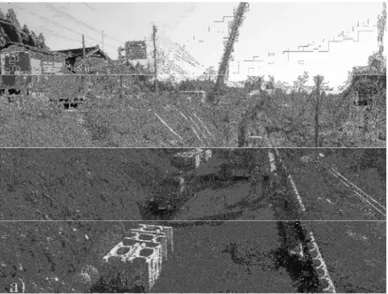
The Higashinada Wastewater Treatment Plant is the City of Kobe’s largest plant, providing one third of the city’s treatment capacity. A location map is shown in Figure 2.10. The facility was heavily damaged when the seawall along the south side of the plant adjacent to the channel moved as much as 3m towards the water as a result of liquefaction. As a result of the movement, the entire site settled an average of one meter. The seawall on the north moved up to 1m south. Liquefaction induced lateral spread and settlement were most sever within a distance of 100m south of the seawall along the southern margin of the channel. Horizontal displacements of 3m and settlements as large as 2 m were observed within the plant site.

(32)

Doctoral Thesys in Geotechnical Engineering , G. Li Destri Nicosia Figure 2.10 Higashinada Wastewater Plant Site Plan

Figure 2.11 Retaining wall along the Inlet between the Island and the mainland moved toward the water (north) 2 to 3 m

(33)

2.5 Retaining wall damage from the Kocaeli (Izmit) Earthquake 1999, Turkey.

In 1999, Turkey was struck by a destructive earthquake the occurred on the western extension of the 1500 km long North Anatolian Fault (NAF). The earthquake hit the most densely populated urban environments, namely Kocaeli and Sakarya provinces, situated on an alluvial fan at the western part of the NAF with magnitude (Mw) 7.4. It also provided some of the

most extensive strong ground motion data set ever recorded in Turkey within about 130 Km of the surface fault rupture.

Surface faulting propagated eastward , starting form the Marmara region, while damaging the transportation infrastructure such as viaduct, bridges, bridge approaches and roadways such as the Trans European Motorways (TEM). At several locations westward of the town of Arifiye, the surface fault intersected the TEM and the bridge overpass in Arifiye, located less than 50km eastward of the epicentre collapsed due to tectonic movement along the fault zone. Beyond the serious collapse of the bridge deck [Pamuk, 2004], the northern bridge approach fill (or ramp) that was reinforced with a pair of mechanically stabilized earth walls (MSEW) was also damaged due to excessive tectonic movement along the fault zone during the main shock of the earthquake. Major damage to the walls was not from seismic design but a combination of adverse effects by the nearby fault movement and, possibly, bearing capacity problems associated with underlying foundation soil.

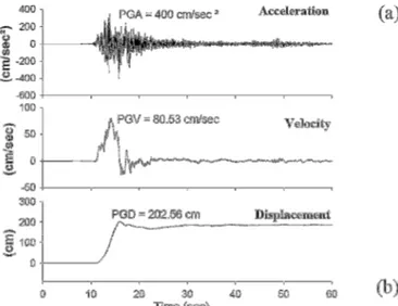
Around 12 people died for a bus passing below the bridge crashed into one the collapsed decks, preliminary repairs cost was around 40 millions dollars and 4% of it was for the demolition and reconstruction of the severely damaged Arifiye Overpass and its reinforced earth abutment system. The closest recording station to the Arifiye Bridge was Sakarya station (SKR), located between downtown Adapazar and Arifiye, for about 4 km northward from the bridge site. The largest peak horizontal ground acceleration of about 0.4g (EW direction) and peak vertical ground acceleration of 0.26g were recorded at this station during the main shock of the Kocaeli earthquake. A clear evidence of impulsive motion (fling) can be observed from the velocity and displacement curves of Figure 2.12

Figure 2.12 Accelerograms recordings at Adapazari station (SKR) and calculated velocity and displacement time histories.

(34)

Unseating of the bridge decks and the damage of the walls of the reinforced approach fill (Figure 2.13, Figure 2.14) were the result of the static displacements due to fault traversing the bridge and its associated strong near-field effects. The presence of the drainage culvert also influences the behaviour of the approach fill. In fact because the vertical displacement at E2 was larger than W2, the approach ramp tilted eastward in the cross section as if the presence of the rigid culvert prevented interaction between the ramp and its foundation, therefore, the walls could not accommodate the underlying ground deformations that was induced by the fault rupture. Beside the panel cracks and separation at these locations, generally speaking the overall performance of the reinforced wall was satisfactory.

Figure 2.13 MSE bridge approach (a) plan view of approach fill with damage concentration; (b) schematic of eastern wall after the earthquake.

(35)

(36)

2.6 Damage to earth structures caused by the 2004 Niigata-Ken Chuetsu Earthquake

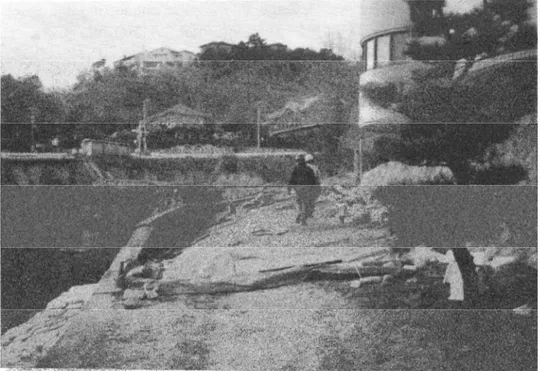
Koseki [Koseki et al, 2005] reports cases in which Embankments and retaining walls for railways, roads and building estates suffered serious damage as a consequence of the 2004 October 23, Niigata-ken Chuetsu earthquake. Such damage was observed at sites where concentration of ground water flow in the subsoil layer may have taken place and/or the fill material may have been partly saturated. River dikes suffered less damage due possibly to less liquefiable conditions of subsoil layers below river dikes in severely-shaken regions. Figure 2.15 shows failure of a gravity type retaining wall along National Highway Route 17 at Kamikatagai, Ojiya city. This wall had been constructed in parallel with a railway embankment, which also suffered from sliding failure Its reconstruction (Figure 2.16) after the earthquake was executed by using the reinforced soil retaining wall with a full height rigid facing.

Figure 2.15 Damage of retaining wall along National Highway Route 17

(37)

2.7 Conclusions

The performance of retaining walls during earthquakes has been found to depend profoundly on the existence of water and the presence of loose cohesionless soils in the supported soil and foundations. Earthquake reality have shown that harbour quay walls made up of either caissons gravity walls or, especially, of passively anchored sheet-pile walls, are quite vulnerable to strong seismic shaking, mainly as a result of strength degradation of saturated cohesionless soils in the backfill and the foundation. This vulnerability was amply demonstrated in the 1995 Kobe earthquake as well as many previous and subsequent earthquakes.

Such behavior [Gazetas et al, 2004] is contrary to the behavior of flexible retaining walls such as the semi-gravity type L-shaped walls, Prestressed-Anchor piled (PAP) walls, and reinforced Soil (RS) walls, retaining non saturated cohesionless soils or saturated clayey soils. These types of walls have behaved particularly (and sometime surprisingly) well during many recent earthquakes as Loma Prieta (1989), Northridge (1994), Kobe (1995), Chi-Chi (1999), Kocalei (1999) and Athens (1999) earthquakes.

(38)

3 FRAMEWORK: ANALYSIS AND DESIGN PRINCIPLES.

Interaction between earth retaining structures and surrounding soil is a complex phenomenon for both static and seismic case. This maybe the main reason for which available analysis-design methods present different degree of complexity as it is difficult to account for all aspects at once. Under static loading it was shown [Rowe, 1957] that wall flexibility leads to important pressure redistribution along the wall and for dense granular fills to consider the effect such redistribution becomes important to accurately evaluate the reduction of bending moment acting on the wall. Presence of anchoring systems may also affect strongly the behaviour of flexible structures in that limiting displacements, anchoring systems may prevent active pressure conditions from developing and elastic soil behaviour modelling maybe appropriate. On the other hand for unanchored structures larger displacements may occur and the occurrence of plastic zones may become important [Faccioli et al., 1996].

In the present chapter a review of available methodologies for the earthquake resistant design of flexible retaining structures is done. Under a didactical point of view it is useful to group different methods depending on specific criteria. A possible classification can be done with respect to the way seismic force is considered. In this case three groups can be identified as follow based on the way seismic input is prescribed:

• Pseudostatic methods: earthquake force is modelled using an equivalent constant additional uniform acceleration as in Monobe-Okabe method [Mononobe and Matsuo,1929] and its variants (e.g. Prakash et al. [1966]). Several solutions based on limit equilibrium (e.g. Rao and Choudhury [2005]), limit analysis (e.g. Lancellotta [2007]) or method of characteristics (e.g. Sokolwskii, [1965]) are available.

• Pseudo-dynamic methods: in which the effect of the input accelerogramm is considered in a simplified way. For flexible retaining structures this approach can be divided in two: either based on rigid block method [Newmark, 1965] as maybe the case of Towata and Islam [1987] where emphasis is put on displacement analysis or subgrade reaction method as the case of Richards et al. [1999].

• Complete dynamic analysis: imply the integration of the equation of motion considering the complete input accelerogramm. Solution can be analytical as the one of Veletsos and Younan [1994a, 1994b, 1997, 2000], Wood [1973], Scott [1973] or

(39)

numerical based on Finite Element Methods (FEM) as the case of Psarropoulos et al, [2005], Madhabushi and Zeng [2006 and 2007] or Finite Difference Method (FDM) as the case of Green and Ebeling [2002].

Another classification can be done with respect to the retaining structure displacements and correlated soil material modelling assumptions:

• Limit state analysis: in which relative soil-wall motion is high enough to lead to soil yielding. A failure mechanism occurs. Example is given by Mononobe-Okabe method [Mononobe and Matsuo,1929] and its variants.

• Linear elastic analysis: where limited wall-soil movement allows for linear elastic assumption. Example are given by Wood [1973], Scott [1973], Veletsos and Younan [1994a, 1994b, 1997,2000].

• Intermediate cases: where non linear soil material behaviour is allowed but no failure mechanism is assumed a priori. This is the case of Richards et al. [1999], or Siller et al. [1991] as well as the case of numerical solutions based on FEM of FDM as above. In the following paragraphs the different approaches will be examined starting from pseudostatic as it is the most used (and sometimes abused) method. Finally tentative conclusions regarding the advantage and limitations of each method will be outlined.

3.1 Pseudostatic approach.

In this paragraph the pseudostatic approach for seismic design of (flexible) earth retaining structures is introduced. Special consideration is given regarding the displacement required for formation of rupture mechanisms and several solutions approaches are presented.

3.1.1 Active and Passive Lateral Earth Pressure: static case

Vertical or near-vertical slopes of soil are supported by retaining walls, cantilever sheet-pile walls, sheet pile bulkheads, braced cuts and other similar structures. The proper design of those structures requires and estimation of lateral earth pressure which is a function of several factors such as the type and amount of wall movement, the strength parameters of the soil, the unit weight of the soil and the drainage conditions in the backfill. A very intuitive definition of active and passive state can be made with reference to wall-soil movement as is shown in Figure 3.1

(40)

Experimental results showing evidence of active thrust and passive resistance for a gravity wall is shown in Figure 3.2. Stress paths in the q-p plane for a granular soil element going from at rest conditions to active state or passive state are shown in Figure 3.3

Figure 3.2 Movement of "soil" surrounding model retaining wall [Lambe, T.W., Whitman, V. W, 1979]

Figure 3.3 Stress paths from at rest conditions to active or passive state [Lambe, T.W., Whitman, V. W, 1979]

Considering (Figure 3.4 a) a horizontal surface of semi-infinite mass of cohesionless soil with a unit weight γ, at depth z below AB, the vertical pressure below ab is p0= γ·z. After deposition of this mass of soil, the value of the lateral earth pressure ph corresponds to the at

(41)

rest value ph= p0=K0·pv. Since the element is symmetrical with respect to the vertical plane, the normal stress on ab is a principal stress. In Figure 3.4d representing the stress state in the plane, the at-rest condition corresponds to circle I.

Figure 3.4 (a) At rest conditions (b,c) Rankine’s states of plastic equilibrium illustrating active conditions (d) Mohr stress and strength diagrams (e,f illustrating passive conditions) [Prakash, S., 1981]

As the soil mass stretches (Figure 3.4a), plane cc moves to the left to position c1c1, lateral pressure decreases and (Figure 3.4d) the diameter of the stress circle increases. According to the MohrCoulomb failure criteria, the greatest diameter that a MohrCircle can have is when the Mohr Circle (II) is tangential to the Mohr strength envelope. The origin of planes is Op,

and OpF1 and OpF2 are failure planes inclined at 45º+φ’/2 each, to the major principal planes.

A relationship between major and minor principal stresses at incipient failure is given by

φ

sin 1 sin 1 + − = = v h a P P K (3.1)

Where Ka is the coefficient of active earth pressure. Once the soil mass stretches and lateral earth pressure reduces to active conditions, further stretching of the mass has no effect on ph

(42)

and sliding occurs along planes parallel to OpF1 and OpF2. The vertical traces of such planes

shown in Figure 3.4c, constitute the shear pattern.

If the wall face is smooth and vertical and deformation conditions for plastic equilibrium is satisfied, the above concepts regarding plastic equilibrium can be applied to determine the active thrust on retaining walls and similar problems.

Similarly if the soil mass is compressed and section cc moves to c2c2, the Mohr Coulomb

circle corresponding to this state of stress is shown by circle III (Figure 3.4, d). Failure planes are in directions of Op’F3 and Op’F4 and are inclined 45º-φ’/2 with respect to the horizontal.

The shear pattern is sketched in Figure 3.4 f and the ratio between vertical and horizontal principal stresses at incipient failure is given by

φ

sin 1 sin 1 − + = = v h p P P K (3.2)

Once again it is noted that once the passive Rankine passive resistance has been mobilized, further compression of the soil causes no increase in soil resistance and slippage occurs along the failure planes.

The strain or relative displacement (∆H/H) required for mobilization of limit states changes depending whether it is active or passive state and depends also on the type of soil. In Figure 3. 5 results of triaxial tests on dry granular soil [Lambe, Whitman 1979] show that the strain level required in order to achieve full mobilization of active state in dense sand is around -0.5% while full mobilization of passive resistance requires around 2% strain.

Figure 3. 5 Strains required to reach passive and active state in dense sand [Lambe, T.W., Whitman, V. W, 1979]

(43)

Consequently, as outlined by Clough and Duncan [1991], the magnitude of relative displacement (∆H/H) required for mobilization changes accordingly and can be assumed for loose sand of the order of 1% for passive case and 0.1% for active case.

Figure 3.6 Nature of variation of lateral earth pressure [Das B.M. , 2007]

Similar values are indicated by EC7 1997 and 2003.

A different approach from the one discussed so far was proposed in 1776 by Coulomb [1776] for calculating the lateral earth pressure on an earth retaining wall with granular soil backfill. Later the method was extended to more general configurations by Mueller-Breslau [1924]. Coulomb methods does not assume neither vertical nor smooth wall but still assumes that the failure surface of the soil is plane.

The solution method is based on global limit equilibrium method and is based on the following steps:

1) finding by trial and error the inclination of a plane failure surface which maximises earth pressure on the wall.

2) assuming a stress distribution along such surface and its resulting force.

3) solution of the problem by mean of global equilibrium of the soil wedge (considered as a rigid body) inside the failure surface.

For a wall as the one showed in Figure 3.7 a) the force triangle is shown in Figure 3.7 b).

(44)

The active state corresponds to the failure surface designated by a value of the angle Ө1 for which the active pressure Pa is maximum. The value of active pressure found by Coulomb is the following: a a H K P = ⋅ ⋅ 2⋅ 5 . 0 γ (3.3)

Where the coefficient of active pressure Kais

(3.4)

and reduces to the value found by Rankine theory based on local stress considerations, for the case of vertical frictionless wall and horizontal backfill. Analogous considerations in the case of passive pressure (see Figure 3.8) lead to the following results

Figure 3.8 Coulomb’s passive pressure [Das B.M. , 2007]

p p H K P = ⋅ ⋅ 2⋅ 5 . 0

γ

(3.5)

Where the coefficient of passive pressure Kpis

2 (3.6) 2 2 ) ( ) ' ( ) ' ( ) ' ' ( 1 ) ' ( ) ' (       + ⋅ + + ⋅ + − ⋅ + ⋅ − =

α

β

δ

β

α

φ

δ

φ

δ

β

φ

β

sin sin sin sin sin sin sin K_p 2 2 2 2 ) ( ) ' ( ) ' ( ) ' ' ( 1 ) ' ( ) ' (         + ⋅ − − ⋅ + + ⋅ − ⋅ + =

β

α

δ

β

α

φ

δ

φ

δ

β

φ

β

sin sin sin sin sin sin sin Ka

(45)

The method is not exact for several reasons such as that none of the continuum generalized equations is satisfied inside or outside the failure surface where rigid body assumption is assumed. Moreover a fundamental assumption in Coulomb’s approach is the acceptance of plane failure surface. The nature of actual failure surface in the soil mass for active and passive pressure for non smooth wall is shown in Figure 3.9 for a vertical wall with horizontal fill. In both active (a) and passive (b) case following a curved part (CD) a plane part (BC) is present.

Although the differences between Coulomb plane surface and the actual surface, for the active case are not so important, in the case of passive pressure Terzaghi [1943] has shown that for smooth walls, the rupture surface is planar and for values of the wall friction angle δp>φ/3, where

φ is the soil friction angle, only curved rupture surfaces should be assumed in the

analysis for the passive case under static condition. As the value of δp increases, Coulomb’s method gives increasingly erroneous values of Pp and lead to an unsafe condition.

In the static case the passive earth pressure problem has been solved by a number of researchers using different techniques such as limit equilibrium with the choice of either planar [Coulomb, 1776] or curved surfaces [Terzaghi, 1943; Caquot and Kerisel, 1948], limit analysis [Chen, 1990] and the method of characteristics [Sokolowski, 1960].

Figure 3.9 Nature of failure surface in soil with wall friction (a) active pressure (b) passive pressure [Das, 2007]

(46)

Doctoral Thesys in Geotechnical Engineering , G. Li Destri Nicosia 3.1.2 Active Lateral Earth Pressure: dynamic case

Coulomb’s theory has been modified by Mononobe-Okabe [Mononobe and Matsuo, 1929] by considering the contribution of the inertia force to the soil wedge equilibrium in the determination of total earth pressure.

In Figure 3.10 a retaining wall of height H and inclined vertically at an angle α retains dry soil with unit weight γ, an angle of shearing resistance φ and a wall friction δ. For a trial failure surface bc1, the inertia force may act on the assumed failure wedge abc1 both horizontally and vertically. Given vertical (av) and horizontal (ah) accelerations of the wedge of soil, the

corresponding inertial forces (W1·ah/g and W1·ah/g) can be assumed, in the worst condition,

acting horizontally toward the wall and vertically in both directions.

Assuming the following definition for the horizontal and vertical seismic coefficient kh and kv

(3.7) (3.8)

Figure 3.10 Active earth pressure under earthquake load (a) force on failure wedge (b) forces polygon [Prakash, S., 1981]

The forces acting on the wedge abc1 (Figure 3.10) maybe listed as follows: 1- W1: weight of the wedge abc1 acting at its centre of gravity

2- P1: earth pressure inclined at an angle δ with respect to the normal of the wall 3- R1 soil reaction, inclined at an angle φ with respect to the normal to the face bc1 4- W1· αh, acting at the centre of gravity of the wedge abc1

5- ±W1· αv, vertical inertia force The angle between the resultant

− + ± ⋅ = 2 2 0.5 1 1 W ((1 k_v) k_h ) W is vertically inclined at an

angle Ө such that

(3.9) ) 1 ( tan 1 v h k k ± = −

ψ

h h _k g a = v v _k g a =

On seismic design and advanced numerical modelling of flexible cantilever walls under earthquake loading including cyclic mobility