19- GUIDE TO SERVO MOTOR SIZING

(1)

A Comprehensible Guide to Servo Motor Sizing

By Wilfried Voss

Published by

Copperhill Technologies Corporation 158 Log Plain Road

Greenfield, MA 01301

No part of this publication may be reproduced, stored in a retrieval system or transmitted in any form or by any means, electronic, mechanical, photocopying, recording, scanning or otherwise, except as permitted under Sections 107 or 108 of the 1976 United States Copyright Act, without the prior written permission of the Publisher.

ISBN: 978-0-9765116-1-8

Printed in the United States of America

Limit of Liability/Disclaimer of Warranty

While the publisher and author have used their best efforts in preparing this book, they make no representations or warranties with respect to the accuracy or completeness of the contents of this book and specifically disclaim any implied warranties or merchantability or fitness for a particular purpose. No warranty may be created or extended by sales representatives or written sales materials. The advice and strategies contained herein may not be suitable for your situation. You should consult with a professional where appropriate. Neither the publisher nor author shall be liable for any loss or profit or any other commercial damages, including but not limited to special, incidental, consequential, or other damages.

(2)

About this book

After years of developing servo motor sizing programs for Windows I deemed it necessary to document the motor sizing process beyond the regular help files. The result of this idea is this book.

My bible for motor sizing and the inertia/torque calculation of mechanical components has been for years a faded copy of “The Texonics Motion Cheat Sheet”, which was given to me by Mr. Charles Geraldi and for which I will be forever grateful. Years later I received a similar version, “The Smart Motion Cheat Sheet” by MSI Technologies, Inc., which was created by Brad Grant, P.E. I am sure, somebody knows the story of how the motion cheat sheet was originally developed and how it evolved. It is so far the most effective written tool for motor sizing that I am aware of.

Both versions of the motion cheat sheet contain on only a few pages everything I needed to know to create the first version of a motor sizing software under MS-DOS and then under the various Windows versions. The result of all these activities is VisualSizer-Professional™, the most advanced motor sizing software in the business. Many businesses in the motion control industry have chosen to use VisualSizer and have it customized for their purposes.

Through the cooperation with many motion control experts I learned that the servo motor sizing process is a somewhat universal procedure. The calculation of inertia and torque of mechanical components, i.e. the motor load, has not changed since the invention of the electrical motor. All the motor has to do is to match the speed, inertia and torque requirements. However, written works on in-depth motor sizing, besides frequent, but somewhat superficial articles in various motion control publications, are extremely rare.

The motor sizing process involves a number of mathematical equations, which are most certainly documented, but not necessarily with the motor sizing process in mind. This book focuses primarily on servo motor sizing, not on motor technologies and other related specifics. It documents the inertia and torque calculation of standard mechanical components and the motor selection process.

Last, but not least, let me re-iterate a previous statement: The calculation of mechanical loads goes way back to the time when Isaac Newton described the three laws of motion. The math of calculating mechanical loads have not changed since then and they did not change with the use of electrical motors. It may be that mechanical components became more sophisticated, but, again, that did not change the way we calculate their inertia and torque.

(3)

About the author

Wilfried Voss is the President of Copperhill Technologies Corporation, a company specializing in motor sizing software development for various motor manufacturers all over the world. In addition, Copperhill Technologies sells user licenses of its generic motor sizing program, VisualSizer-Professional™. Since 2005 the product offering has been extended to include technical literature on all aspects of motion control and fieldbus technologies.

Mr. Voss has been involved with motion control applications since 1985 as a specialist in the paper industry and in addition, since 1997, is also involved with fieldbus technologies, especially CAN (Controller Area Network) related technologies. He has a master's degree in electrical engineering from the University of Wuppertal in Germany. Mr. Voss has traveled the world extensively, settling in New England in 1989. He presently lives in an old farmhouse in Greenfield, Massachusetts with his Irish-American wife and their son Patrick.

Acknowledgements by the author

This book would never have been possible without the vision of Mr. Charles Geraldi, then Sales Manager at Parvex Servo Systems in New York, who in 1992 hired me to develop a motor sizing software for MS-DOS and Windows 3.1. “Not expensive!” he wrote on the two pages from a notepad, which represented the entire outlining of the software. At the time I had done some motion controller programming, but had never heard of motor sizing.

Another collaborator in this coupe d’etat on my person was Edward Crofton, then President of Automation & Servo Technologies, who, in cooperation with Charles Geraldi, was one of my biggest supporters for many years. No one could have imagined that this afternoon meeting in 1992 would lead to creating the most successful software package of its kind. Thanks, guys!

Also thanks to those experts who provided their support and knowledge and helped to make VisualSizer a success: Both John M’s of Baldor Motor and Drives, i.e. John Malinowksi and John Mazurkiewicz, for their kind support and for showing me the best BBQ place in the world (a little shed in Oklahoma).

Thanks also to Paul Derstine of GE Fanuc, a vigorous tester of my program, Craig Ludwick and Nick Johantgen of Oriental Motors U.S.A., Uwe Krauter of Siemens Energy & Automation, Meng King of AC Tech

(4)

Contact the author

As the disclaimer on the very first page explains in the required legal English: “While the publisher and author have used their best efforts in preparing this book, they make no representations or warranties with respect to the accuracy or completeness of the contents of this book and specifically disclaim any implied warranties or merchantability or fitness for a particular purpose.”

We are aware of the vast number of experts in the industry and we are sure that some of them would like to see specific topics explained in more detail or even consider some topics not being represented properly. For all those who would like to contribute constructive criticism or would like to add more insights that involve the servo motor sizing process, please feel free to contact us!

We have set up a “Contact the Author” section under http://www.copperhilltech.com/ServoSizingBook/. We encourage you to send your comments!

Please understand that we cannot respond to requests asking for help on how to handle your specific application needs.

(5)

Chapter

1

Overview

he vast majority of automated manufacturing systems involve the use of sophisticated motion control systems that, besides mechanical components, incorporate electrical components such as servo motors, amplifiers and controllers.

The first straightforward task for the motion system design engineer, before tuning and programming the electrical components, is to specify – preferably the smallest - motor and drive combination that can provide the torque, speed and acceleration as required by the mechanical set up.

However, all too often engineers are familiar with the electrical details, but do lack the knowledge of how to calculate the torque requirements of the driven mechanical components. In other cases they try to size their application around the motor and spend valuable time to figure out how to move the load under the given circumstances. Such an approach will lead to improperly sized motion control applications. The impact, economically as well as technically, will be one of the topics in the following chapters.

Modern motor sizing software packages, such as VisualSizer-Professional™, provide the convenience of computing all necessary equations and selecting the optimum motor/drive combination within minutes; they are, however, mainly used to circumvent the timely process of selecting a motor manually. While motor sizing programs can have an educational value to some degree, most of them do not provide any reference on how the equations were derived.

Some basic knowledge of inertia and torque calculations can have a profound impact on the motion system performance. Simple details, like when to use a gearbox in a motion system, may not only help to reduce costs, but will most certainly improve the system performance.

The following chapters will provide a comprehensive insight into the motor sizing process including detailed descriptions of inertia and torque calculations of standard mechanical components.

(8)

Chapter

2

The Importance of Servo Motor Sizing

he importance of servo motor sizing should not be underestimated. Proper motor sizing will not only result in significant cost savings by saving energy, reducing purchasing and operating costs, reducing downtime, etc.; it also helps the engineer to design better motion control systems.

2.1 Why Motor Sizing?

The servo motor represents the most influential cost factor in the motion control system design, not only during the purchasing process, but especially during operation. A high-torque motor will require a stronger and thus more expensive amplifier than smaller motors. The combination of higher torque motor plus amplifier results not only in higher initial expenses, but will also lead to higher operational costs, in particular increased energy consumption. It is estimated, that the purchase price represents only about 2% of the total life cycle costs; about 96% is electricity.

Picture 2.1.1: Lifecycle costs of an Electrical Motor

(9)

The conventional method of servo motor sizing is based on calculations of the system load, which determines the required size of a motor. Standard praxis demands to add a safety factor to the torque requirements in order to cover for additional friction forces that might occur due to the aging of mechanical components. However, the determination of the system load and the selection of the right servo motor can be extremely time consuming. Each motor has its individual rotor inertia, which contributes to the system load torque, since Torque equals Inertia times Acceleration. The calculation of the system torque must be repeated for each motor that is being considered for the application.

As a result, it is not an easy task to select the optimum motor for the application considering the vast amount of available servo motors in the marketplace. Many motors, that are currently in action, have been chosen mostly due to the fact that they are larger than required and were available short-term (e.g. from inventory). The U.S. Department of Energy estimates that about 80% of all motors in the United States are oversized.

The main reasons to oversize a motor are:

¾ Uncertain load requirements

¾ Allowance for load increase (e.g. due to aging mechanical components) ¾ Availability (e.g. inventory)

Not only is the power consumption higher than it should be; there are also some serious technical considerations.

2.2 Technical Aspects

Oversizing a motor is naturally more common than undersizing. An undersized motor will consequently not be able to move the load adequately (or not at all) and, in extreme cases, may overheat and burn out, especially when it can’t dissipate waste heat fast enough. Larger motors will stay cool, but if they are too large they will waste energy during inefficient operation. After all, the motor sizing process can also be seen as an energy balancing act.

AC motors tend to run hot when they are loaded too heavily or too lightly. Servo motors, either undersized or oversized, will inevitably start to vibrate or encounter stalling problems.

One of the major misconceptions during the motion design process is that selecting a larger motor than required is only a small price to pay for the capability to handle the required load, especially since the load

(10)

Picture 2.2.1: Example Efficiency vs. Load

Picture 2.2.1 shows an example of two motors, 10 HP and 100 HP. In both cases there is a sharp decline of the motors’ efficiency at around 30% of the rated load.

However, the curves as shown in the picture, will vary substantially from motor to motor and it is difficult to say when exactly a motor is oversized. As a general rule of thumb, when a motor operates at 40% or less of its rated load, it is a good candidate for downsizing, especially in cases where the load does not vary very much. Servo motor applications usually require short-term operation at higher loads, especially during acceleration and deceleration, which makes it necessary to look at the average (RMS) torque and the peak torque of an application.

There are, however, advantages to oversizing:

¾ Mechanical components (e.g. couplings, ball bearings, etc.) may, depending on the environment and quality of service, encounter wear and as a result may produce higher friction forces. Friction forces contribute to the constant torque of a mechanical set up.

¾ Oversizing may provide additional capacity for future expansions and may eliminate the need to replace the motor.

(11)

High efficiency motors, compared to standard motors, will maintain their efficiency level over a broader range of loads (see picture 2.2.2) and are more suitable for oversizing.1

Picture 2.2.2: Example High/Low Efficiency Motors

2.3 The Objective of Motor Sizing

The main objective of motor sizing is based on the good old American sense for business: Get the best performance for the lowest price. As we have learned from a previous chapter the lifecycle costs of an electrical motor are:

¾ Purchasing Costs – 2%

¾ Repair, Service, Maintenance, etc. – 2% ¾ Operating Costs (Electricity) – 96%

In order to get the best performance for the best price it is mandatory to find the smallest motor that fulfills the requirements, i.e. the motor that matches the required torque as close as possible. The basic assumption (which is true for the majority of cases) is that small torque is in direct proportion to smaller size, lower costs and lower power consumption. Smaller power consumptions also result in smaller drive/amplifier size and price.

(12)

From a technical standpoint it is also desirable to find a motor whose rotor inertia matches the inertia of the mechanical setup as close as possible, i.e. the optimum ratio between load to rotor inertia of 1 : 1. The inertia match will provide the best performance. However, for servo motors a ratio of up to 6 : 1 still provides a reasonable performance. Any higher ratios will result in instabilities of the system and will eventually lead to total malfunction.

In many cases it makes sense to add a gear between motor and the actual load. A gear lowers the inertia that is reflected to the motor in direct proportion of the transmission ratio. This scenario allows to run smaller motors, however, with the price of the gear added to the system. On the other hand the price reduction by using a smaller motor/drive combination may more than just compensate for the gear’s price.

In review the objective of motor sizing is to:

¾ Get the best performance for the best price

¾ Match the motor’s torque with the load torque as close as possible ¾ Match the motor’s inertia with the load inertia as close as possible ¾ Find a motor that matches or exceeds the required speed

(13)

Chapter

3

The Motor Sizing and Selection Process

he motor sizing and selection process is based on the calculation of torque and inertia imposed by the mechanical set up plus the speed and acceleration required by the application. The selected motor must be able to safely drive the mechanical set up by providing sufficient torque and velocity.

Once the requirements have been established, it is easy to look either at the torque vs. speed curves or motor specs and choose the right motor.

The sizing process involves the following steps:

1. Establishment of motion objectives 2. Selection of mechanical components 3. Definition of a load (duty) cycle 4. Load calculation

5. Motor selection

1. Establishment of motion objectives

A written outlining of the motion control application will help to establish the necessary parameters needed for the next steps.

¾ Required positioning accuracy ? ¾ Required position repeatability ? ¾ Required velocity accuracy ? ¾ Linear or rotary application ?

¾ If linear application: Horizontal or vertical application?

(14)

2. Selection of mechanical components

The engineer must decide which mechanical components are required for the application. For instance, a linear application may require a leadscrew or a conveyor. For speed transmission a gear or a belt drive may be used.

¾ Direct Drive ?

¾ Special application or standard mechanical devices ?

¾ If linear application: Use of linear motor or leadscrew, conveyor, etc. ? ¾ Reducer required – Gearbox, belt drive, etc. ?

¾ Check shaft dimensions – select couplings

¾ Check mechanical components for speed and acceleration limitations

3. Definition of a load (duty) cycle

The engineer must define the maximum velocity, maximum acceleration, duty cycle time, acceleration and deceleration ramps, dwell time, etc., specific to the application.

¾ Define critical move parameters such as velocity, acceleration rate ¾ Triangular, trapezoidal or other motion profile ?

¾ If linear application: Make sure the duty cycle does not exceed the travel range of linear motion device.

¾ Jerk Limitation required ? ¾ Consideration of thrust load ?

¾ Does the load change during the duty cycle ? ¾ Holding brake applied during zero velocity ?

4. Load calculation

The load is defined by the torque that is required to drive the mechanical set up. The amount of torque is determined by the inertia “reflected” from the mechanical set up to the motor and the acceleration at the motor shaft.

¾ Calculate inertia of all moving components ¾ Determine inertia reflected to motor

(15)

5. Motor Selection

The motor must be able to provide the torque required by the mechanical set up plus the torque inflicted by its own rotor. Each motor has its specific rotor inertia, which contributes to the torque of the entire motion system. When selecting a motor the engineer needs to recalculate the load torque for each individual motor.

¾ Decide the motor technology to use (DC brush, DC brushless, stepper, etc.) ¾ Select a motor/drive combination

¾ Does motor support the required maximum velocity ? If no, select next motor/drive.

¾ Use rotor inertia to calculate system (motor plus mechanical components) acceleration (peak) and RMS torque

¾ Does motor’s rated torque support the system’s RMS torque? If no, select next motor/drive.

¾ Does motor’s intermittent torque support the system’s peak torque? If no, select next motor/drive.

¾ Does the motor’s performance curve (torque over speed) support the torque and speed requirements? If no, select next motor/drive.

¾ If the ratio of load over rotor inertia exceeds a certain range (for servo motors 6:1) consider the use of a gearbox or increase the transmission ratio of the existing gearbox. Servo motors should not be operated over a ratio of 10:1.

As mentioned earlier, a modest oversizing of the motor of up to 20% is absolutely acceptable. The oversizing factor should be implemented during the torque requirement checks. In this case it also acceptable to use a higher factor for the acceleration (peak) torque.

The motor selection process as described also explains the popularity of motor sizing programs. The process of recalculating the torque requirements for each individual motor/drive combination can be extremely time consuming considering the vast amount of motors available in the industry. The goal of motor sizing is to find the optimum motor for the application and that can only be accomplished with sufficient choices available, i.e. with a great number of applicable motors.

(16)

(17)

The following chapters will explain the steps between ‘Selection of mechanical components’ and ‘Motor Selection’ in more detail, supported by a sample application.

3.1 Selection of mechanical components

The engineer must decide which mechanical components are required for the application. For instance, a linear application may require a leadscrew or a conveyor. For speed transmission a gear or a belt drive may be used.

¾ Direct Drive ?

¾ Special application or standard mechanical devices ?

¾ If linear application: Use of linear motor or leadscrew, conveyor, etc. ? ¾ Reducer required – Gearbox, belt drive, etc. ?

¾ Check shaft dimensions – select couplings

¾ Check mechanical components for speed and acceleration limitations

The most common mechanical components for a motion application are:

¾ For speed transmissions: ¾ Gear

¾ Belt Drive

¾ Chain Drive (Chain-Sprocket)

¾ For linear movements: ¾ Conveyor

¾ Leadscrew ¾ Linear Actuator2

¾ Rack-Pinion

¾ For other purposes: ¾ Coupling ¾ Brake ¾ Encoder

(18)

¾ Other applications: ¾ Rotary Table ¾ Nip Roll ¾ Winders ¾ Hoist

While a detailed functional description of these components is not in the scope of this book, it is nevertheless mandatory for motor sizing and selection to document the corresponding inertia and torque calculations. For detailed information on these calculations refer to Chapter 4 – Load Inertia and Torque Calculations. The knowledge of how to calculate inertia and torque of these components will also help in the calculation of more complex mechanical units.

In the following we will examine a very simple mechanical application, i.e. a motor and a disk as shown in the picture below.

Picture 3.1.1: Disk Application

A disk actually represents the majority of motor load components, i.e. when you can calculate the inertia of a disk you can do the same for a leadscrew, conveyor, belt pulley, and many other loads. Screws, pulleys, gears, etc. can be seen as disks and hence use the same inertia equations.

(19)

Sample Application: Disk Application

1

The motion objective of this sample application shall be to accomplish a trapezoidal motion profile, i.e. to accelerate the disk to a certain speed, hold the speed for some time and then decelerate to zero speed again.

The disk shall be 2” in diameter, 1.2” in thickness. The material shall be steel, which has a material density of 0.28 lbs/in3_.

(20)

3.2 Definition of a load cycle

A load cycle, i.e. the way the actual motion is applied, can have numerous shapes. There are, for instance, simple applications like blowers, conveyor drives, pumps, etc. that inflict only constant or gradually changing torque over a very long time. Sizing a motor for these applications is fairly simple and does not require further processing of the motion cycle. This book is primarily concerned with servo applications, which require abrupt and frequent torque changes during the load cycle.

The simplest forms of servo load cycles are triangular and trapezoidal motion profiles (as explained on detail in the following chapters). They define the most critical data such as maximum speed and maximum acceleration and they are sufficient enough to cover the majority of motion applications and subsequent determination of the torque requirements. Naturally there are also very complex motion profiles and their detailed processing will result in more precise determination of the RMS torque requirement, while the peak (intermittent) torque requirement depends mainly on the maximum acceleration inside the motion cycle.

In order to process the load cycle the engineer must define the maximum velocity, maximum acceleration, duty cycle time, acceleration and deceleration ramps, dwell time, etc., specific to the application.

¾ Define critical move parameters such as velocity, acceleration rate ¾ Triangular, trapezoidal or other motion profile ?

¾ If linear application: Make sure the duty cycle does not exceed the travel range of linear motion device.

¾ Jerk Limitation required ? ¾ Consideration of thrust load ?

¾ Does the load change during the duty cycle ? ¾ Holding brake applied during zero velocity ?

There are two basic (and very similar) types of a motion profile (duty/load cycle):

¾ Triangular Motion ¾ Trapezoidal Motion

(21)

3.2.1 Triangular motion profile

Picture 3.2.1.1 demonstrates the triangular motion profile:

Picture 3.2.1.1: Triangular Motion Profile

Symbol Description

v Velocity

vmax Maximum Velocity

t Time

ta Acceleration Time

td Deceleration Time

t0 Dwell Time (Time at zero speed)

The motor accelerates to the maximum velocity and then immediately after reaching the maximum decelerates towards zero. Depending on the application the motor may remain at standstill for some time.

(22)

3.2.2 Trapezoidal motion profile

Picture 3.2.2.1 demonstrates the trapezoidal motion profile:

Picture 3.2.2.1: Trapezoidal Motion Profile

v Velocity

vmax Maximum Velocity

t Time

tc Constant Time

ta Acceleration Time

td Deceleration Time

t0 Dwell Time (Time at zero speed)

The motor accelerates to the maximum velocity, holds that velocity for some time and then decelerates towards zero. Depending on the application the motor may remain at standstill for some time.

For non-horizontal linear applications, i.e. moving the load in an angle up or down, it is important to consider the use of a holding brake. The motor needs to compensate for the

(23)

3.2.3 Motion profile processing

The following equations are universal between triangular and trapezoidal motion profiles, considering that a triangular motion profile behaves like a trapezoidal motion profile without the constant time (time at constant speed).

In order to calculate the torque requirements we need the following data from the motion profile:

¾ RMS Torque

¾ Total cycle time

¾ Acceleration/Deceleration time

¾ Constant time (time at constant speed; will be zero for triangular profile) ¾ Dwell time (time at zero speed)

¾ Peak (Intermittent) Torque

¾ Maximum Acceleration/Deceleration (Torque = Inertia times Acceleration)

The duty cycle parameters for the determination of the RMS torque can naturally be derived directly from the motion profile. The maximum acceleration is calculated as shown below:

(24)

In order to determine the maximum acceleration/deceleration it is necessary to use the absolute amount of the deceleration, since deceleration is basically a negative acceleration. The maximum torque will occur during the highest acceleration/deceleration.

In case that a more complex motion profile is required, the engineer will need to process all time segments in order to calculate the RMS torque. To calculate the peak (intermittent) torque the engineer needs to record the acceleration/deceleration of each time segment and determine the maximum acceleration from these values as shown in the next example.

Picture 3.2.3.2: Acceleration calculation for complex motion profile

Some applications may require different deceleration ramps, for instance, one for regular deceleration (regular stop command) and one for emergency operation (emergency stop command). In such a case the emergency stop deceleration may determine the highest torque requirement.

(25)

The following picture demonstrates the difference between a triangular and a trapezoidal motion profile in terms of torque requirements.

Picture 3.2.3.3: Torque during Triangular and Trapezoidal Motion Profile

Both motion profiles use the same total cycle time. The trapezoidal profile, however, requires a higher acceleration/deceleration rate, which in turn results in higher torque requirements. This circumstance can be of importance for some motion control applications.

Sample Application: Calculation of Maximum Load Acceleration

2

The motion profile shall be of trapezoidal shape using the following parameters: ta = td = 1 sec

tc = 2 sec

t0 = 1 sec

vmax = 1000 rpm = 16.67 rev/sec

(26)

3.2.4 Motion profile calculation

The following chapter provides some more insight into the calculation of the motion profile in a more generic sense. The equations as shown here are based on the use of radians for traveled distance, radians/sec for speed and radians/sec2_{for acceleration and deceleration.}

Picture 3.2.4.1: Trapezoidal Motion Profile

Symbol Description Angular unit Rotational unit

ω Velocity rad/sec rps or rpm

ωmax Maximum Velocity “ “

α

Acceleration _rad/sec2_rev/_sec2

Θ Distance (rotation) rad rev

Θa Distance (rotation) during acceleration “ “

Θc Distance (rotation) during constant speed “ “

Θd Distance (rotation) during deceleration “ “

t Time sec sec

(27)

The equations for trapezoidal moves are:

⎟

⎠

⎞

⎜

⎝

⎛

₊

×

=

+

=

2

max a c d d c a Total

t

ω

θ

⎟

⎠

⎞

⎜

⎝

⎛

₊

=

2

max d c a Total

t

θ

ω

Equation 3.2.4.1: Trapezoidal Moves

The equations for triangular moves (with tc = 0) are:

⎟

⎠

⎞

⎜

⎝

⎛

₊

×

=

+

=

2

max a d d a Total

t

ω

θ

⎟

⎠

⎞

⎜

⎝

⎛

₊

=

2

max d c a Total

t

θ

ω

With ta = td: a Total

t

θ

ω

_max

=

Equation 3.2.4.2: Triangular Moves

(28)

(

ω

)

_π

α

₌

max

−

0

_×

2

a

t

Equation 3.2.4.3: Acceleration calculation

ω0 represents the initial angular or rotational velocity. With ω0 = 0 the equation changes to:

π

ω

α

₌

max

_×

2

a

t

Equation 3.2.4.4: Acceleration calculation with ω0 = 0

Naturally, there are motion applications that require a more complex load cycle and subsequent processing of the motion profile, which in turn has major implications on the load torque. These applications include, for instance, vertical movements, jerk limitation (S-Curve), etc. which will be explained later in more detail. For educational purposes it seemed to be necessary to cover the basics before engaging into more sophisticated mathematical models.

(29)

3.2.5 Motion profile equations

Parameter Description English Engineering Metric

θ

Rotation rev rad

ω

Velocity rev/sec, rpm rad/sec

t Time sec sec

α

Acceleration rev/sec2_rad/sec2

Unknown Known Equation

α

ω

₀

,

t

,

₍

₎

2

2 0

at

t

+

×

=

ω

θ

t

,

₀ max

ω

₍

₎

2

0 max

t

×

+

=

ω

θ

α

ω

_max

,

₀

,

α

ω

θ

×

−

=

2

2 0 2 max

θ

[radians]

α

ω

_max

,

t

,

₍

₎

2

2 max

t

−

×

=

ω

α

θ

α

ω

₀

,

t

,

ω

_max

=

ω

₀

+

(

α

×

t

)

t

,

ω

₀

θ

0 max

2 θ

_ω

ω

=

×

−

t

α

ω

θ

,

₀

,

_ω

₌

_ω

2

₊

₍

₂

_×

_α

_×

_θ

₎

0 max max

ω

[rad/sec]

α

θ

,t

,

2

max

t

×

+

=

θ

α

ω

α

ω

_max

,

t

,

ω

₀

=

ω

_max

−

(

α

×

t

)

t

,

ω

_max

θ

max 0

2 θ

_ω

ω

=

×

−

t

α

ω

θ

,

_max

,

_ω

₌

_ω

2

₋

₍

₂

_×

_α

_×

_θ

₎

max 0 0

ω

[rad/sec]

α

θ

,t

,

2

0

t

×

−

=

θ

α

ω

α

ω

_max

,

₀

,

α

ω

_max

−

₀

=

t

t [sec]

(30)

Unknown Known Equation 0 max

,

ω

θ

ω

α

×

−

=

2

2 0 2 max

t

,

₀ max

ω

t

0 max

ω

α

=

−

t

,

ω

₀

θ

⎟

⎠

⎞

⎜

⎝

⎛

₋

×

=

t

0 2

2 θ

ω

α

[rad/sec2_]

t

,

ω

_max

θ

⎟

⎠

⎞

⎜

⎝

⎛

₋

×

=

₂

max ₂

t

θ

ω

α

(31)

3.2.6 Jerk Limitation

Jerk Limitation (a.k.a. S-Curve Profiling) is the time rate of change of axis acceleration/deceleration. It provides smoother motion control by reducing the jerk (rate of change) in acceleration and deceleration portions of the motion profile.

Its purpose is to eliminate mechanical jerking when speed changes are made and can be used to minimize mechanical wear and tear, optimizing travel response, reduce splashing when transporting liquids, prevent tipping when transporting boxes on a conveyor, etc.

Without jerk limitation With jerk limitation (100%) Picture 3.2.6.1: Speed and Torque Profile

Jerk limitation is defined as a percentage of each deceleration and acceleration segment. This percentage is then equally divided between the beginning and end of the segment. For example, for an acceleration

(32)

Without jerk limitation With jerk limitation (100%) Picture 3.2.6.2: Velocity and Acceleration

Picture 3.2.6.2 demonstrates clearly the difference in acceleration between linear acceleration (no jerk limitation) and S-Curve profiling (with jerk limitation).

Jerk Limitation increases the torque requirements and may result in a need for a larger motor, i.e. larger jerk factors require a larger peak torque from the motor. For example, a segment with 100% jerk limitation requires twice the peak (acceleration) torque as the same segment using linear acceleration.

The following series of pictures shows a comparison of different jerk limitation percentages and the resulting torque requirements:

(33)

Picture 3.2.6.3: 0% Jerk Limitation

Note that a value of 0% results in a linear motion and torque profile. The intermittent (peak) torque requirement in this example is not quite 8 in-lbs.

This is the same example as shown previously, but in this case with a jerk limitation of 50%. The effects of the jerk limitation are visible. Note that the torque profile shows a trapezoidal shape. Also note that the intermittent torque requirement is slightly higher than in the previous picture, i.e. a little over 8 in-lbs.

(34)

Picture 3.2.6.5 shows the effects of 100% jerk limitation (using the same sample application as the previous pictures). Note that the torque profile shows a triangular shape. Also note the significantly higher torque requirements of roughly 11 in-lbs.

Be aware that the previous sample application requires a constant torque of roughly 3 in-lbs. The previous statement that 100% jerk limitation requires twice the peak torque than a linear acceleration remains true.

Last, but not least, picture 3.2.6.6 demonstrates why the intermittent torque requirements are higher with jerk limitation:

(35)

The jerk limited motion profile requires a higher acceleration and deceleration rate than the linear profile and higher acceleration/deceleration results directly into higher torque.

3.2.6.1 S-Curve Calculation

The following equations are based on the assumption that the area under an acceleration vs. time graph is the equivalent of the velocity, since v = a x t. Let’s have a look at the acceleration ramp of a sample S-Curve and its resulting acceleration graph.

Picture 3.2.6.1.1: Acceleration ramp

(36)

The final velocity based on picture 3.2.6.1.1. can be calculated as follows:

2

max

t

a

v

_f

=

×

vf Final Velocity

amax Max. Acceleration

t Total Acceleration Time

Equation 3.2.6.1.1: S-Curve Final Velocity

However, in order to cover all possible jerk limitation percentages we need to look at a different acceleration curve. The following picture demonstrates a generic acceleration ramp.

t1 Time of Increasing Acceleration

t2 Time of Constant Acceleration

t3 Time of Decreasing Acceleration

t1 = t3 = 0 Jerk Limitation = 0%

(37)

Picture 3.2.6.1.2 shows an acceleration ramp that represents roughly a 60% jerk limitation. As was explained previously, the percentage is equally divided between the beginning and end of the segment. For example, for an acceleration segment of 1 second and a jerk limitation of 60%, the first 30% (from 0 to 0.3 seconds) and last 30% (from 0.7 to 1 second) of the segment include jerk limitation. A value of zero is used for linear acceleration.

Based on this definition of the jerk percentage it can be safely assumed that t1 and t3 have equal values. The

final velocity for the generic S-Curve acceleration ramp can be calculated as follows:

2

3 max 2 max 1 max

t

_a

_t

a

t

a

v

_f

=

×

+

×

+

×

With t1 = t3: 2 max 1 max

t

a

t

a

v

_f

=

×

+

×

)

(

₁ ₂ max

t

a

v

_f

=

×

+

Equation 3.2.6.1.2: S-Curve Final Velocity (Generic)

The next assumption is that the motion control engineer tends to define the maximum velocity for a given application and that, in order to create a velocity profile, the equations should provide the information of the velocity at any given time.

With the final velocity vf known and also assuming that the acceleration/deceleration ramp times are known

we can now calculate the maximum acceleration.

2 1 max

t

v

a

f

+

=

(38)

In the following we need to look at three different sections of the acceleration ramp (See also picture 3.2.6.1.2):

• Increasing Acceleration • Constant Acceleration

• Decreasing Acceleration (Deceleration)

1. Increasing Acceleration:

0 ≤

t

≤

t

₁

1. Acceleration at any given time t:

1 max

t

a

=

×

2. Velocity vt at any given time t:

2 t

a

v

_t

=

×

2

1 max

t

a

v

_t

×

=

1 2 max

2 t

t

a

v

_t

×

=

(39)

2. Constant Acceleration:

t

₁

≤

t

≤

(

t

₁

+

t

₂

)

max

a

=

2. Adjust time: 1

t

=

−

t

a

t

a

v

_t

=

max

×

1

+

_max

×

2 ⎟

⎠

⎞

⎜

⎝

⎛ +

×

=

a

t

v

_t

2

1 max

(40)

3. Decreasing Acceleration (Deceleration):

(

t

₁

+

t

₂

)

≤

t

≤

(

t

₁

+

t

₂

+

t

₃

)

⎟⎟

⎠

⎞

⎜⎜

⎝

⎛

−

×

=

3 max

1 t

t

a

2. Adjust time: 2 1

t

=

−

2

max 1 max

t

_a

_t

a

t

a

v

_t

=

×

+

×

+

×

2

1

2

3 max max 1 max

t

a

t

a

t

a

v

_t

×

⎟⎟

⎠

⎞

⎜⎜

⎝

⎛

−

×

+

×

+

×

=

⎟⎟

⎟

⎠

⎞

⎜⎜

⎜

⎝

⎛

−

+

×

=

2

3 2 2 1 max

t

a

v

_t

(41)

Last, but not least, let’s accomplish some calculations of a sample application profile in order to prove the validity of the previously described equations.

The sample profile is based on the following parameters:

Max Velocity 1000 rpm Acceleration Ramp Time 100 msec Jerk Limitation 50% t1 25 msec t2 50 msec t3 25 msec

Max. Acceleration 13.33 rev/msec2 _{(Calculated; see equation 3.2.6.1.3)}

0.00 200.00 400.00 600.00 800.00 1000.00 1200.00

(42)

The calculated velocity points are as follows (based on 2.5 msec increments): t vt 1. Increasing Acceleration 0 0.00 2.5 1.67 5 6.67 7.5 15.00 10 26.67 12.5 41.67 15 60.00 17.5 81.67 20 106.67 22.5 135.00 25 166.67 2. Constant Acceleration 27.5 200.00 30 233.33 32.5 266.67 35 300.00 37.5 333.33 40 366.67 42.4 400.00 45 433.33 47.5 466.67 50 500.00 52.5 533.33 55 566.67 57.5 600.00 60 633.33 62.5 666.67 65 700.00 67.5 733.33 70 766.67 72.5 800.00 75 833.33 3. Decreasing Acceleration: 77.5 865.00 80 893.33 82.5 918.33 85 940.00 87.5 958.33 90 973.33 92.5 985.00 95 993.33 97.5 998.33 100 1000.00

(43)

3.3 Load calculation

The load of a motor is determined by its own rotor inertia, the total inertia reflected from the mechanical set up, the constant torque from the mechanical set up, and the maximum speed and maximum acceleration of the application.

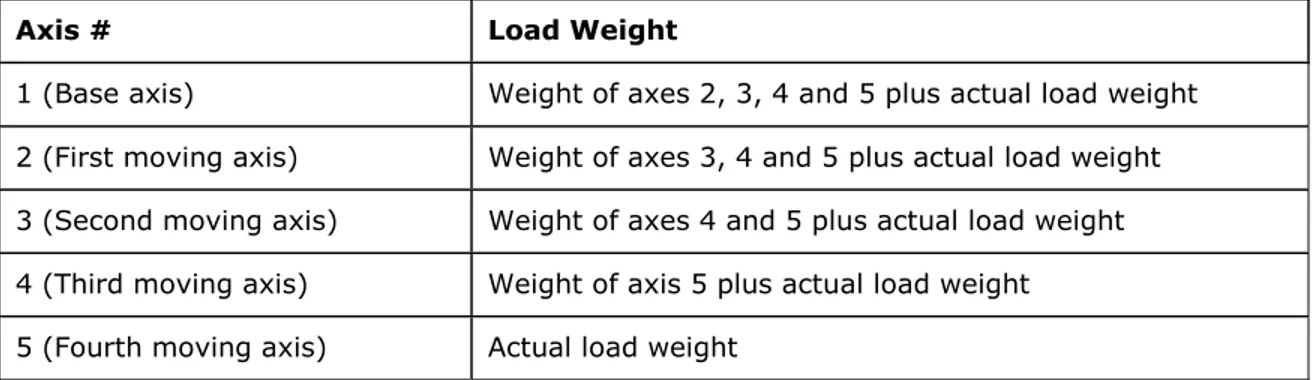
As demonstrated in the following picture any calculation of the load parameters starts with the last mechanical component in the set up.

Picture 3.3.1: Motor load

The speed, acceleration, inertia and constant torque is “reflected” from mechanism to mechanism until it reaches the motor. Each component will add its own inertia and constant torque. Speed transmission components, like, for instance, a gear, will also transform the inertia, speed and acceleration from the previous component according to the transmission ratio.

The total (system) inertia and the maximum acceleration will determine the acceleration torque. The total torque, i.e. the required peak (intermittent) torque is the sum of acceleration torque and constant torque.

The required RMS torque result from the entire motion cycle and the acceleration and constant torque of each motion segment as will be explained in more detail later in this chapter.

(44)

The following picture explains the process in more detail using the same sample application:

Picture 3.3.2: Motor load transmission

The basic required data to select a motor are:

¾ Load maximum speed

¾ Load maximum (intermittent) torque ¾ Load RMS (rated) torque

(45)

The following shows an excerpt from a report created with VisualSizer-Professional. The application comprises of a motor, a servo reducer and a leadscrew. The leadscrew moves a weight of 3 lbs.

Selected Motor :

Manufacturer AutomationDirect.Com Product Family SVL - Low Inertia Motors Product Key SVL-204

Drive Module SVA-2040

Rated Speed 3000 rpm Rated Torque 11.236 in-lb Max. (Peak) Torque 33.798 in-lb Rotor Inertia 0.00030082 in-lb-s² Kt 0 in-lb/A Motor Load Data :

Max. Velocity 3000 rpm Constant Torque 2.8353 in-lb RMS Torque 5.2295 in-lb Peak Torque 10.525 in-lb Load Inertia 0.00247237 in-lb-s² Ratio Load/Rotor Inertia 8.2188 : 1 System Data (incl. Rotor Inertia) :

RMS Torque 5.7357 in-lb Peak Torque 11.46 in-lb Total Inertia 0.00277319 in-lb-s² Mechanism No. 1 : Right-Angle Servo Reducer

Manufacturer SHIMPO DRIVES, INC. Product Key NEVKFE15P20019011LR Reducer Ratio 15 : 1 Moment of Inertia 0.002472 in-lb-s² Internal Losses 2.777 in-lb Reducer Efficiency 92 % Weight 27.6 lb Nominal Output Torque 956 in-lb Max. Output Torque 1744 in-lb Max. Input Speed 5000 rpm Calculated Input Shaft Load Data :

Max. Input Velocity 3000 rpm Total Inertia 0.00247237 in-lb-s² Mechanism Inertia 0.002472 in-lb-s² Constant Torque 2.8353 in-lb Peak Torque 10.525 in-lb Calculated Output Data :

(46)

Screw Diameter 0.35 in Screw Length 25 in Material Density 0.28 lb/in³ Pitch / Lead 25 rev/in Mechanism Efficiency 96.8 % Friction Coefficient 0.11 Preload Torque 0.8 in-lb Thrust Forces 0 lb Table Weight 2.7 lb Angle 0 °

Coupling Inertia 0.00005 in-lb-s² Max. Velocity 0 rpm Calculated Input Shaft Load Data :

Max. Input Velocity 200 rpm Total Inertia 0.00007733 in-lb-s² Mechanism Inertia 0.000027 in-lb-s² Constant Torque 0.804124 in-lb Peak Torque 0.820157 in-lb Load Parameters :

Type Weight Only Weight 3 lb

The calculation of the motor load is accomplished as follows:

1. Add load weight to the leadscrew table weight.

2. Calculate the screw inertia and add the table & load inertia reflected to the input shaft. 3. Apply the resulting inertia as load inertia to the servo reducer.

4. Add the servo reducer inertia plus the load inertia reflected to the input shaft and apply it to the motor.

In order to apply speed and acceleration to the motor shaft take into account the transmission ratio (or lead/pitch) of each device.

(47)

As was mentioned earlier, there are simple applications like blowers, conveyor drives, pumps, etc. that inflict only constant or gradually changing torque over a very long time. Sizing a motor for these applications is fairly simple and does not require any complex processing of the motion cycle. To size a motor for this kind of application it is only necessary to match the load torque, which is usually accomplished by matching the load with the motor’s horsepower using the following equation: [ ] [ ] [ ]

₅₂₅₀

rpm ft lb HP

v

T

P

=

×

− 1 HP = 746 Watts = 550 ft-lb/sec

3.3.1 Load maximum speed

The maximum speed is naturally directly acquired from the motion profile as demonstrated in an example below, where v2 represents the maximum speed.

(48)

In regards to the sample application we apply the maximum speed as shown below.

Sample Application: Determination of Maximum Load Speed

3

As defined in the motion profile the maximum required speed is:

vmax = 1000 rpm

3.3.2 Load inertia and maximum torque

The calculation of the maximum (intermittent) torque is fairly easy, since it depends mainly on the maximum acceleration. However, the maximum torque contains of two components:

1. Constant torque as inflicted by the mechanical setup. This is the torque due to all other non-inertial forces such as gravity, friction, preloads and other push-pull forces.

2. Acceleration torque as inflicted by the inertia3_{from the mechanical setup plus the maximum}

acceleration as required by the load cycle.

Be aware that, during the motor selection process, the motor’s rotor inertia must be added to the load inertia.

(49)

Picture 3.3.2.1: Example of acceleration and constant torque

The equations used to calculate the maximum torque are:

rotor app system

J

=

+

a

J

T

_a

=

_system

×

c a total

T

=

+

Equation 3.3.2.1: Determination of maximum torque

Jsystem Total system inertia

Japp

Application inertia (inflicted by mechanical setup)

Jrotor Rotor inertia

(50)

For the sample application we apply the following:

Sample Application: Calculation of Intermittent/Peak Torque

4

Max. acceleration amax = 16.67 rev/sec2 as derived from the motion profile.

The inertia of the disk is determined as:

Disk Weight:

π

⎟

×

ρ

⎠

⎞

⎜

⎝

⎛

×

=

D

L

W

2

Disk Inertia:

g

r

L

g

r

W

J

_disk

×

=

×

=

2

4 2

_π

_ρ

Using the disk dimensions as defined earlier the disk inertia will be:

2

0.00137

sec

disk

J

=

in lb

− −

In the following we assume a rotor inertia of 0.0011 in-lb-sec2_.

2

0.00137 0.0011 0.00247

sec

system

J

=

+

=

in lb

− −

Since a disk does not inflict any friction, we assume the constant torque to be zero. As a result the acceleration torque represents the total torque:

2

0.259

a total system

T

=

T

=

J

× × × =

α

π

in lb

−

Symbol Description W Weight ∏ “PI” = 3.14159 D Disk diameter

L Disk thickness (length)

ρ Material density

(51)

The calculation of the disk’s inertia as demonstrated with the sample application provides a first glimpse into the inertia calculation of, in this case, a basic component. The calculation of, for instance, the inertia of a leadscrew, a rotary table, a pulley, etc. is based on the same math as shown here.

3.3.3 Load RMS torque

While the calculation of the maximum (intermittent) torque is fairly easy, the calculation of the RMS load torque is a bit more complex. The RMS torque (“Root Mean Squared”) represents the average torque over the entire duty cycle. To calculate the RMS torque the following parameters are required:

¾ Torque during acceleration ¾ Torque during constant speed ¾ Torque during deceleration ¾ Acceleration time

¾ Time of constant speed ¾ Deceleration time ¾ Holding time

(52)

The following picture demonstrates the determination of these parameters:

Picture 3.3.3.1: Demonstration of torque and time segments

Ta Total torque during acceleration (incl. constant torque)

Tc Constant torque due to friction

Td Total torque during deceleration (incl. constant torque)

ta Acceleration time

tc Time of constant speed

td Deceleration time

th Holding time

(53)

The equation to calculate the RMS torque is as shown below:

(

)

2 2

(

)

2 2 a c a c c d c d h h RMS a c d h

T

t

T

t

T

t

T

t

T

t

+

× +

+

× +

×

=

+ + +

Equation 3.3.3.1: RMS torque calculation

Symbol Description Ta Acceleration torque Tc Constant torque Td Deceleration torque Th Holding torque ta Acceleration time

th Holding time

Ta, Tc , Td and Th as shown in the equation represent absolute values. Deceleration

torque is usually negative. The motor, however, has to provide at least that amount of torque to drive the mechanical setup during deceleration.

The equation can be simplified for a triangular motion profile (not considering the constant time tc) as follows:

(

)

2

(

)

2 ₂ a c a d c d h h RMS a d h

T

t

T

t

T

t

T

t

+

× +

+

× +

×

=

+ +

(54)

The calculation of the acceleration and deceleration torque is achieved the same way as during the peak torque calculation, however, in this case the calculation has to be accomplished for each individual motion segment. a system d system

T

J

T

J

d

α

=

×

=

×

Equation 3.3.3.3: Determination of accel. / decel. torque

Symbol Description

Jsystem Total system inertia4

Ta Acceleration torque

a Acceleration

Td Deceleration torque

d Deceleration

Acceleration means in this case angular acceleration. Angular acceleration is measured in radians per sec2_.

The constant torque, i.e. the torque due to all other non-inertial forces such as gravity, friction, preloads and other push-pull forces, must be derived from component data sheets (e.g. a leadscrew’s preload torque) or application specifics (refer to Chapter 4 – Load Inertia and Torque Calculations).

(55)

Things become a bit more tedious in cases where a motion profile more complex than triangular or trapezoidal is required as demonstrated in the following picture.

(56)

Sample Application: Calculation of RMS Torque

5

The equation to calculate the total RMS torque for a trapezoidal motion profile, including load and motor inertia, is:

(

)

2 ₂

(

)

2 ₂ a c a c c d c d h h RMS a c d h

T

t

T

t

T

t

T

t

T

t

+

× +

+

× +

×

=

+ + +

By applying our current sample application data, i.e. assuming the constant torque to be zero and acceleration/deceleration times are 1 sec, the equation can be simplified to the following:

(

)

2 2 2

_{2 0.259}

0.164

5

a d RMS a c d h

T

in lb

t

×

+

=

−

+ + +

Symbol Description Ta Acceleration torque Tc Constant torque Td Deceleration torque Th Holding torque ta Acceleration time

(57)

3.4 Motor Selection

The motor selection process, as demonstrated in picture 3.4.1, can be initiated as soon as all load parameters have been established.

(58)

The motor selection process as described here also explains the popularity of motor sizing programs. The process of recalculating the torque requirements for each individual motor/drive combination can be extremely time consuming considering the vast amount of motors available in the industry. The goal of motor sizing is to find the optimum motor for the application and that can only be accomplished with sufficient choices available, i.e. with a great number of applicable motors.

3.4.1 Matching Motor Technologies to Applications

Prior to the actual selection process based on inertia, speed and torque comparisons, it makes sense to decide which motor technology might be best suited for the application. This method will limit the number of motors that need to be investigated and thus will reduce the time it takes to find the optimum motor.

Just as a reminder: This book is not intended to explain the basics of electrical motors. There are numerous works available on this topic. This book merely addresses the topic of motor sizing and selection. It is nevertheless necessary to address in brief the characteristics of motor technologies as they do have some bearing on the motor selection process.

The motor technologies commonly used for servo applications are:

¾ Stepper ¾ DC Brush

¾ DC Brushless (Permanent Magnet) ¾ Synchronous AC

¾ Asynchronous AC (AC Induction)

The DC Brushless and Synchronous AC technologies are actually identical; some manufacturers prefer to call it DC Brushless, others rather use Synchronous AC.

(59)

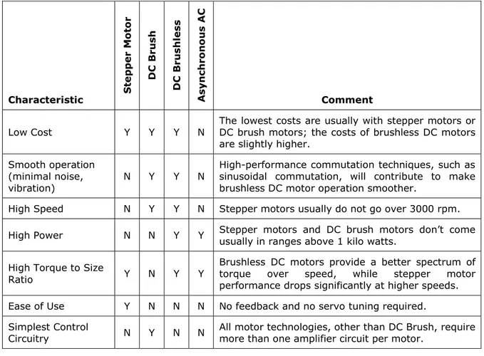
Table 3.4.1.1 provides an overview of the motor technologies and their basic operating characteristics: Characteristic Ste ppe r Mo to r DC Brus h DC Brus hl e ss As y n chro no us AC Comment

Low Cost Y Y Y N The lowest costs are usually with stepper motors or DC brush motors; the costs of brushless DC motors are slightly higher.

Smooth operation (minimal noise,

vibration) N Y Y N

High-performance commutation techniques, such as sinusoidal commutation, will contribute to make brushless DC motor operation smoother.

High Speed N Y Y N Stepper motors usually do not go over 3000 rpm. High Power N N Y Y Stepper motors and DC brush motors don’t come _{usually in ranges above 1 kilo watts.}

High Torque to Size

Ratio Y N Y Y

Brushless DC motors provide a better spectrum of torque over speed, while stepper motor performance drops significantly at higher speeds. Ease of Use Y N N N No feedback and no servo tuning required. Simplest Control

Circuitry N Y N N All motor technologies, other than DC Brush, require more than one amplifier circuit per motor.

Table 3.4.1.1: Motor Technology Characteristics

3.4.1.1 Stepper Motors

Stepper motors are basically DC brushless motors. They are self-positioning and they do not require an encoder for position feedback. However, some applications may use an encoder for the sole purpose of detecting “stall” during motion.

Stepper motors produce a high torque for a given size and weight. However, the available torque from stepper motors drops dramatically with higher speed and the complex performance curves (torque over speed) complicate the selection for a specific application. Their maximum speed is in the neighborhood of 5000 rpm

(60)

The major drawback of stepper motors is the noise and vibration they produce. Especially vibration can effect the lifetime of a mechanical system significantly. There are, however, measures to reduce vibration such as microstepping drive techniques or mechanical dampers, but they usually do not eliminate the problem completely.

3.4.1.2 DC Brush Motors

DC Brush motors are suitable for a wide variety of applications, especially for positioning, but also for speed and torque control. They do require an encoder for positioning applications.

DC Brush motors are available in a great variety of sizes, up to several kilo watts. The speed range can be as high as 10,000 rpm and even higher. They run smoothly and relatively quiet.

The major disadvantage of DC Brush motors are the brushes, which do wear out over time and need to be replaced. They can also be responsible for electrical arcing.

Another drawback is that DC Brush motors provide a relatively low torque in comparison to their size and weight.

3.4.1.3 DC Brushless Motors

Just like the DC Brush motor the DC Brushless motor requires an encoder for position feedback. It is, however, the most widely used motor technology for servo applications. Brushless DC motors run relatively smooth and quiet; they do not require mechanical brushes for commutation.

Due to excellent thermodynamic features it is able to generate high torque for a given size. DC Brushless motors are available in a wide power range and they can operate at very high speeds up to 30,000 rpm and even more.

The drawback of a DC Brushless motor can be its high price due to the use of rare-earth magnetic materials to generate torque. They also require fairly complex and thus more expensive amplifiers.

19- GUIDE TO SERVO MOTOR SIZING

A Comprehensible Guide to Servo Motor Sizing

About this book

About the author

Acknowledgements by the author

Contact the author

Table of Contents

Chapter

1

Overview

Chapter

2

The Importance of Servo Motor Sizing

Chapter

3

The Motor Sizing and Selection Process

1

2

α

⎟

⎠

⎞

⎜

⎝

⎛

+

+

×

=

+

+

=

2

2

t

t

t

ω

θ

θ

θ

θ

⎟

⎠

⎞

⎜

⎝

⎛

+

+

=

2

2

t

t

t

θ

ω

⎟

⎠

⎞

⎜

⎝

⎛

+

×

=

+

=

2

2

t

t

ω

θ

θ

θ

⎟

⎠

⎞

₊

₊

₊

₊

₊

₊

₊

_π

₌

_×

₌

_×

₍

₎

₍

₎