Department of Computer, Control and Management Engineering University of Rome La Sapienza
Ph.D. Program in
Automatic control, Bioengineering and Operations Research Curriculum: BIOENGINEERING
XXXII Cycle
The structural and functional multilayer modular
organization of the human brain
Maria Grazia Puxeddu
Advisor
Laura Astolfi, Ph.D.
Co-advisor
Manuela Petti, Ph.D.
Ph.D. program coordinator
Giuseppe Oriolo, Ph.D.
External reviewers
Christian-G. Bénar, Ph.D.
Richard F. Betzel, Ph.D.
Academic Year 2019/2020Tables of contents
Introduction ... 1
Hints of brain connectivity and graph theoretical analysis ... 5
i. Structural and functional brain connectivity ... 5
ii. Network science applied to brain imaging ... 8
iii. The modular structure of brain networks ... 9
SECTION I - Comparison among multilayer community detection algorithms and application to EEG-based functional connectivity ... 13
1.1. Introduction ... 13
1.2. Methods ... 18
1.2.1. Benchmark networks generation ... 18
1.2.2. Simulation studies for algorithms comparison ... 21
1.2.3. Multilayer community detection on EEG brain networks ... 26
1.3. Results ... 27
1.3.1. Simulation studies for algorithms comparison ... 27
1.3.2. Multilayer community detection on EEG brain networks ... 35
1.4. Discussion ... 37
1.5. Conclusion ... 41
1.6. Supplementary material ... 42
1.6.1. Comparative analysis on networks with evolving community structure and increasing or decreasing clusters number ... 42
1.6.2. Comparative analysis on networks with lower graph density ... 47
1.6.3. Preliminary investigation on the temporal resolution parameter in the multilayer modularity optimization algorithm, genlouvain ... 52
1.6.4. Preliminary investigation on the trade-off parameter in the multi-objective function optimization algorithm, FacetNet ... 57
SECTION II - The modular organization of the human brain networks across the lifespan ... 62
2.1. Introduction ... 62
2.2. Methods ... 64
2.2.1. Experimental dataset and data processing ... 64
2.2.2. Multilayer network construction ... 65
2.2.4. Analysis of the communities ... 68
2.3. Results ... 71
2.3.1. Statistics of the multilayer multiscale modularity maximization ... 71
2.3.2. Age-related changes of the modular structure ... 74
2.4. Discussion ... 81
2.5. Conclusion ... 87
SECTION III - The modular organization of the human brain networks across functional and structural connectivity and across subjects ... 88
3.1. Introduction ... 88
3.2. Methods ... 90
3.2.1. Experimental dataset and data processing ... 90
3.2.2. Multi-modal multi-subject community detection ... 92
3.2.3. Analysis of the communities ... 94
3.2.4. Correlation with behavioral assessments ... 97
3.3. Results ... 99
3.3.1. Preliminary analysis of the communities ... 100
3.3.2. Modes of variability between and within modality ... 103
3.3.3. Variability between and within modalities at specific scales ... 106
3.3.4. Correlation with behavioral assessments ... 111
3.4. Discussion ... 115
3.4.1. Relationship between structural and functional modular structure across subjects ... 115
3.4.2. Methodological innovations of the multilayer framework ... 117
3.4.3. Limitation and future advancements ... 118
3.5. Conclusion ... 119
Conclusion ... 120
Bibliography ... 123 List of publications
1
Introduction
The human brain is an embedded complex system whose functions cannot be reduced to the processes of its fundamental units. Rather, brain functioning emerges as a consequence of complex patterns of interactions involving all its parts at different levels, from neuron cells to larger brain areas.
The past years have been characterized by exponential growth in the field of neuroimaging techniques. Hence the availability of large datasets that characterize brain interactions patterns (Jirsa and McIntosh, 2007), crossing different domains and time-scales, or associated with task-evoked brain activity. The need for robust methods to interpret and manage the increasing complexity and size of these data nicely met the rise of network science (Börner et al., 2007; Newman, 2010). Indeed, the intersection of these disciplines led to the modeling of the brain as a network, in which a number of nodes (subcortical, cortical or scalp regions) interact each other through a set of edges (structural or functional connections) (Bullmore and Sporns, 2009; Sporns, 2014). Thus, the parallel recording of the interactions of many neuronal groups results in datasets forming, under a mathematical/physics point of view, a complex network. Once the brain network has been estimated, its emerging or topological properties can be measured through a rich collection of metrics developed in the field of network science and rooted in the mathematical branch of graph theory (Bullmore and Bassett, 2011). In this context was born the network neuroscience (Bassett and Sporns, 2017), an ascending discipline aimed to map, synthesize, analyze, interpret and model neurobiological data. Nowadays, network neuroscience forms the backbone of our way to comprehend the brain structure and function as a complex system.
Several measures of the graph theory have been extensively applied to the structural and functional brain networks, in order to investigate their topological properties. In the first instance, neuroscientists exploited local and global measures to assess the importance of single brain regions (nodes) or properties of the network as a whole, respectively, revealing non-random attributes. These measures included for example degree centrality,
2
betweenness centrality, path length, clustering coefficient, and efficiency. However, local and global measures might not paint the whole picture of the brain functioning, so that more recently a new focus has been on the mesoscale (intermediate) level. Here we can observe how the brain network’s elements organize themselves in modules that adopt different configurations basing on the type of connectivity, the brain state, and the external environment. In the network science, modules are groups of nodes internally strongly interconnected, but weakly coupled with the other nodes of the network. By supporting balanced mechanisms of integration and segregation within and between different brain areas (Sporns, 2013), modules constitute the building blocks underpinning brain network’s organization. Thus, decomposing the brain network to identify its modular structure has become crucial to gain new insights into brain cortical organization as well as cognitive functions (Fox and Friston, 2012; Tononi et al., 1994).
The network-based modeling and analysis have profoundly contributed to deepening our understanding of brain functioning. Many times, modules have been detected in single networks, extracting useful information on single subjects, time-points, tasks, disease or connectivity patterns. Yet, there is a long way to go in the inferences across brain networks. Indeed, the patterns of human brain connectivity intrinsically evolve across several domains. Brian networks can change their topology, for example, in time in ranges spanning from milliseconds (thanks to high temporal resolution acquisition techniques based on EEG/MEG) to years (e.g. in lifespan studies). Connectivity patterns might also vary across the frequencies in which the collected signals can be decomposed, across different tasks, from subject to subject, across different acquisition modality, and in turn also the modular structure would mutate. For a long time, two easy strategies adopted to manage this amount of information consisted of aggregating or discarding data, to obtain a single network instance. However, such strategies could be misleading or could lead to poorly accurate or reliable results. The mathematical formalism of multilayer networks addresses this issue (De Domenico, 2017; Kivelä et al., 2014; Vaiana and Muldoon, 2018). A multilayer network consists of an ensemble of single-layer networks, each one corresponding and encoding a specific attribute of the system (i.e. different time points,
3
frequencies, subjects, tasks, connectivity metrics). This formulation combines the simplicity of the classical networks and the flexibility in modeling multimodal data. While many graph measures have been successfully translated from single- to multi-layer networks, principled frameworks are still needed, that could allow to treat and manipulate dependencies in multilayer networks. Overall, the size and complexity of brain data and physiological questions on brain architecture require adequate multilayer frameworks developed upon robust strategies for statistical inference.
In this context takes place this dissertation, which tackles the challenge of uncovering and characterizing modules in multilayer brain networks. It serves a dual purpose. On one side we attempted to broaden our knowledge of the human brain structural and functional organization across different domains, on the other side we enriched the mathematical and statistical methods in the field of multilayer networks.
While the following chapter introduces the principal methods that will be exploited, the main body of this work is composed by three sections, that take the form of journal articles.
In section I, I report a comparative analysis among different algorithms employed to detect modules in multilayer networks. In fact, despite the presence of some common practice, there is still no agreement about which algorithm is the most reliable, and a way to test and compare them all under a variety of conditions is lacking. We tested their ability to recover both steady and dynamic modules configurations, statistically evaluating their performances by means of ad-hoc implemented benchmark graphs. Results seek to provide guidelines about the choice of the more appropriate algorithm according to the different properties of the brain network under exam. To prove the validity of the results, we applied the algorithms to functional brain networks derived from electroencephalographic (EEG) signals in a controlled condition. Despite modular organization has not been really investigated in EEG based brain networks, we believe they are extremely suited to study the evolution of cognitive processes across time, and so through a multilayer framework, given their high temporal resolution.
4
In section II we investigated the evolution of the brain structural modular organization across the human lifespan. In doing that, we developed an ensemble-based multilayer network approach, a statistical procedure that allowed us to efficiently link changes of structural connectivity patterns to development and aging.
Given the results obtained in section I, where we found the best multilayer community detection algorithm, in section III we extended its formulation to track variations of brain network architecture across two domains simultaneously. In particular, we explored how it changes across subjects and across different types of connectivity (structural and functional).
The studies in sections II and III make use of a freely available dataset, released as part of the Nathan Kline Institute (NKI), Rockland, NY lifespan sample. It includes functional, diffusion-weighted, and structural magnetic resonance imaging (MRI) scans of individuals aged 7-85 years, from which we reconstructed structural and functional networks.
A conclusion summarizing the main contributions of this Ph.D. project, together with their impact and limitation, closes this dissertation. Finally, two chapters are dedicated to a list of the papers and CV originated from this Ph.D. course.
Section I has been carried out in collaboration with the Neuroelectrical Imaging and BCI Lab (NEILab, PI: Donatella Mattia, MD, Ph.D.) at Fondazione Santa Lucia, IRCCS, Rome, Italy. All the data threatened in this section have been collected in this laboratory. Sections II and III were performed in collaboration with the Computational Cognitive Neuroscience Laboratory (PI: Olaf Sporns, Ph.D.) and the Brain Networks and Behavioral Laboratory (PI: Richard Betzel, Ph.D.) of Indiana University, Bloomington, USA.
5
Hints of brain connectivity and graph theoretical analysis
i. Structural and functional brain connectivity
Brain connectivity refers to patterns of links connecting distinct units of the central nervous system (Jirsa and McIntosh, 2007; McIntosh and Mišić, 2013). Both elements and links can encode different information. Units can stand for single neuronal cells, neural groups, or larger brain regions. Links can be divided in two main classes: (i) links constituted by anatomical connections, such as synapses or fiber tracts pathways between cortical and subcortical grey matter regions, form structural connectivity; (ii) links inferred through statistical or causal dependencies, such as cross-correlation or coherence, form the functional brain connectivity. In this way, structural connectivity refers to anatomical (physical) connections among brain areas, while functional connectivity to their activity or co-activity over time (Friston, 2011), regardless of whether these areas are connected by direct structural links.
Overall, brain connectivity underpins and constrains brain activity, so that reconstructing and analyze it plays a key role in elucidating brain functioning.
In this dissertation the focus will be on human brain connectivity/networks. While animal nervous system can be sometimes studied through invasive techniques, the human brain is mostly investigated with non-invasive imaging methods, like electroencephalography (EEG), magnetoencephalography (MEG), and magnetic resonance imaging (MRI). EEG and MEG capture rapid variations of the electric and magnetic field generated at cortical level and still observable in the scalp surface. MRI applies specific sequences of magnetic field to excite atoms in the brain. Atoms respond altering properties associated to brain activity, such as blood volume and oxygen concentration. Measuring these alterations is then used to estimate structural and functional connections among brain regions. Here we will exploit brain connectivity estimated from EEG and MRI signals.
6
To reconstruct structural networks we used MRI, that also goes by the name of diffusion weighted imaging (DWI) (Hagmann et al., 2007). DWI exploit the motion of the water molecules in the brain to infer tracts of connections. In a free space water is subjected to Brownian motion that shows no preferential diffusion direction (isotropic motion). In the brain, the presence of myelinated axon bundles constrains the direction of the water motion (anisotropic motion), so that water molecules diffuse preferentially along the bundles’ longitudinal axis (Basser et al., 2000; Mori and Zhang, 2006). Exciting atoms through a magnetic field and estimating the directionality of the caused motion, we can reconstruct physical pathways connecting neural elements, commonly called “streamlines”. The number of streamlines connecting two regions of the cortex surface will constitute the weight of the link connecting these nodes in the brain network. Different processing strategies adopted to obtain the final structural network will be discussed in the studies in section II and III.
MRI scans can also be used to estimate functional connectivity, basing on the concept that neuronal activity is strictly related to blood flow in the brain vessels (Logothetis et al., 2001). Indeed, sustained activity of neuronal populations require oxygen, which is transported and furnished by the hemoglobin contained in red blood cells. Hence, when active, brain areas will by surrounded by oxygen-rich blood. The quantity of oxygen in the blood affects its ferromagnetic properties, so that applying a magnetic field and observing the response of the blood it is possible to distinguish between oxygen-rich (active) and oxygen-poor (non-active) brain areas. The signal observed is called BOLD (blood-oxygen-level-dependent). Functional connectivity can be then inferred by observing the BOLD signal in different brain areas and identifying in which of them it co-fluctuates, exploiting for example measures of correlation. The correlation coefficients of all the pairs of brain regions will constitute the links of the functional brain network. A more detailed preprocessing of the BOLD signals will be treated in section III.
We estimated functional brain networks also from EEG recordings. EEG measures the spontaneous activity of the brain by capturing, through sensors placed on the scalp, the voltage fluctuations resulting from ionic currents provoked by the synchronous activity
7
of pyramidal neurons. From these signals we can infer functional connectivity in terms of directed causal information flow between brain areas. The concept of causality is based on Granger’s argument (Granger, 1969), that if a signal X1 “causes” a signal X2, then the
lagged values of X1 contain information that help in predicting X2 above and beyond the
information contained in the lagged values of X2. Granger causality is statistically
implemented through different methods, including Direct Transfer Function (DTF) (Kaminski and Blinowska, 1991), Partial Directed Coherence (PDC) (Baccalá and Sameshima, 2001) and Phase-slope Index (PSI) (Nolte and Mueller, 2010), that can all be applied to EEG signals. In this thesis we used the PDC metric. PDC is a spectral estimator based on multivariate autoregressive models that allow to reconstruct the direction of information flow. It is known to be characterized by high accuracy in the estimation of connectivity patterns, distinguishing between direct and indirect connectivity flows better than other estimators (Astolfi et al., 2007). More details on the estimation of EEG functional connectivity based on PDC will be discussed in section I.
Both MRI and EEG are well established non-invasive neuroimaging methods. Being able to extract connectivity patterns from both type of signals is crucial, since no one technique by itself can adequately address the varied questions of interest in research and clinical applications. EEG signals are suitable to recover highly variable connectivity patterns, due to its high temporal resolution. Moreover, EEG has the great advantage of being a low-cost, portable technique, which allows to collect data from subjects in a variety of tasks and under different clinical conditions. MRI, on the contrary, suffers of temporal resolution and portability in favor of an excellent spatial resolution, that allows reconstructing brain tissue, and consequently connectivity patterns, at the millimeter level. In the first section, we exploited the high temporal resolution of the EEG, to build a temporal multilayer network in which layers represent timestamps, in order to investigate the community detection algorithms in different condition where connectivity patterns suddenly changed or remained stable across several milliseconds. In the second section, we exploited the MRI high spatial resolution to accurately investigate the structural modular organization of the human brain across the lifespan. Finally, in the third section
8
we exploited MRI signals, to build a new model able to explore the relationship between structural and functional connectivity.
ii. Network science applied to brain imaging
Brain connectivity patterns can be mathematically represented and analyzed in the form of a graph (Bullmore and Sporns, 2009; Bullmore and Bassett, 2011; Fornito et al., 2016). A graph is an abstract representation of a network suitable for every kind of connectivity discussed in the previous paragraphs. It consists of a set of vertices (or nodes) connected each other by means of edges (links, connections). In the following chapter nodes will corresponds to small portion of the cortex (voxels) in MRI based studies, or to larger brain areas subtended by the sensors in EEG recording. The links instead, will correspond to streamlines counts (anatomical connectivity), correlation coefficients (functional connectivity inferred from BOLD signals), or causal interactions (functional connectivity inferred from EEG signals).
Mathematically a graph made of N nodes can be represented through an adjacency matrix A in which the entries aij (with i,j=1,…,N) assumes a value different from zero only
if a link exists connecting node i with node j, and vice versa (Figure 1). The links of the
Figure 0.1. Representation of the brain connectivity through a graph (panel a), the list of nodes and edges (panel b), and the relative adjacency matrix (panel c).
9
graph can be binary or weighted, basing on whether the existence of the link is the only aspect of interest or we are interested in the strength of such connection. Binary and weighted adjacency matrix are made of 0/1 and 0/non-zero entries, respectively. Moreover, links can be directed or undirected basing on whether we know the direction of influences between nodes or it is impossible to determine whether the activity of brain region a influences that of region b or whether it is the other way around. Undirected graphs result in a symmetric adjacency matrix, while this is not necessarily true for the directed one. In this dissertation we will deal with both binary-directed networks (estimated from EEG signals) and weighted-undirected networks (estimated from MRI data).
Modeling connectivity patterns as a network allow us to extract quantitative information from it by means of several indices that can be computed on the graph. Among many others, measures on brain networks many times included the calculation of the node’s degree or strength, clustering coefficient, path length, betweenness or eigenvector centrality, efficiency, small-worldness. All these measures capture local or global properties of the networks, inferring on the centrality/importance of single nodes or global topological properties of the network.
iii. The modular structure of brain networks
This thesis focuses on measures lying at an intermediate level, between local and global, where the organization of the nodes within the network can be observed. Community structure (Newman and Girvan, 2004; Porter et al., 2009) fits this level and consists of the organization of the network in groups of nodes (clusters or communities) promoting mechanisms of segregation and integration between brain areas (Sporns, 2013), that shape communication patterns and make the system efficient. Communities in brain networks (Figure 2) usually refer to groups of nodes in which the network itself can be divided, possibly responsible for specific domains of brain functioning.
10
While many definitions of community exist in network science, brain networks often exhibit assortative communities, composed by groups of nodes internally highly interconnected while poorly connected with the rest of the network. So-made communities are also referred to as modules (Sporns and Betzel, 2016). Modules can be detected in a data-driven way, basing on the topology of the network, and understanding the modules’ composition within the brain network could provide important insights into brain function. To date, many studies have been already carried out detecting modules in anatomical and functional brain networks. In one of the firsts (Hagmann et al., 2008) an anatomical modular structure consisting of six modules has been found, and special attention was put on identifying those regions highly connected intra- and inter-modules, known as hubs. Lately (Heuvel and Sporns, 2013, 2011) those hubs have been found to play a key role in shaping information flow. Other efforts were put on identifying the multiscale organization of anatomical brain networks (Betzel et al., 2013; Lohse et al., 2014), revealing the presence of different meaningful community organization corresponding to cluster of different size. Also in functional network the modular structure has been investigated. First it has been showed that the human brain is actually organized into modules of functionally interconnected areas (Laumann et al., 2015; Meunier et al., 2009). Later it has been found that these communities can be associated to cognitive/behavioral function (Power et al., 2011). Beside a qualitative description of the human brain modular organization, more recent efforts were put on revealing its evolution in different domains. Studies characterized modules composition across
Figure 2. Example of a brain network partitioned into four clusters. The grouping in clusters is indicated through different colors. Intra-clusters and inter-Intra-clusters edges are indicated through continuous and dashed arrows, respectively.
11
cognitive states (Andric and Hasson, 2015; Godwin et al., 2015), during aging (Zuo et al., 2017) (a deeper analysis in section II), or in a learning paradigm (Bassett et al., 2011b). As we will show, multilayer paradigms can be extremely useful in tracking communities in multimodal networks.
There exist different methods to detect community in networks, and through section I we will attempt to provide some guidelines regarding the use of them. In the meanwhile, we want to introduce the popular concept of modularity (Q) (Newman, 2006), a quality function used to assess the goodness of a division of the network into modules. Given a network and a partition of it into nodes, modularity estimates the goodness, in terms of assortativity, of this partition with respect to a null model. Its formulation is reported below, in Eq. 1:
𝑄(𝛾) = ∑[𝑊𝑖𝑗− 𝛾𝑃𝑖𝑗]𝛿(𝜎𝑖𝜎𝑗)
𝑖𝑗
(Eq. 1) Where 𝑊𝑖𝑗 and 𝑃𝑖𝑗 are the actual and expected weights of the connection linking nodes
i and j. The variable 𝜎𝑖 ∈ {1, …, K} indicates to which cluster node i belongs, and 𝛿(𝑥, 𝑦) is
equal to 1 if 𝑥 = 𝑦 and 0 otherwise. The parameter γ represents a spatial resolution weight that, scaling the importance of the null model 𝑃𝑖𝑗, rewards partitions with few or many
modules. Many possible definitions of null model exist. One of the most common is the configuration model 𝑃𝑖𝑗 =
𝑘𝑖𝑘𝑗
2𝑚, in which each node’s connection strength is preserved but
edges are placed in a random fashion.
A multilayer version of Q has been recently introduced (Mucha et al., 2010), in order to qualify assortative communities in multilayer networks. This version allows to incorporate a second channel of connectivity, which in multilayer brain networks can represent for example time or subjects. Its formulation is given by:
𝑄(𝛾, 𝜔) = ∑[(𝑊𝑖𝑗𝑟 − 𝛾𝑃𝑖𝑗𝑟)𝛿𝑟𝑡+ 𝜔𝛿𝑖𝑗]𝛿(𝜎𝑖𝑟𝜎𝑗𝑡)
𝑖𝑗𝑟𝑡
(Eq. 2)
Here nodes are linked to themselves across layers through the temporal resolution parameter ω. Its value weights the similarity of the partitions across layers (indicated
12
through r and t), so that high (low) ω-values reward (non) homogeneous partitioning across layers.
I introduced from the beginning these concepts of modules, modularity and multilayer modularity because they constitute the focus of this Ph.D. project, and will be recurrent over each section.
iv.
Validation of network’s indices
However, before getting to the heart of the dissertation, I want to highlight that the use of every complex network measure should be accompanied by the design of some null hypothesis. If a null model is properly designed, the statistical comparison of the indices computed on the actual and the null model could provide significant insights on the topological properties of the complex system under exam. Null models are not universally defined. Usually they are built preserving and randomizing different properties, according to the features of interest. In single layer networks, for example, when the focus is on the centrality of the nodes a frequently used null model consists of randomizing edges while preserving the degree-distribution. In absence of a null model, statistical frameworks are needed that ensure the reliability of the obtained measure. The validation of the network’s indices through null models or robust statistics also applies to multilayer networks. For example, when the order of the layers is important (i.e. time-varying networks), is a common practice comparing the indices obtained on the real network with those obtained with the multilayer network in which layers are randomly permuted, but networks properties are preserved within each layer. In each of the following section the measures obtained will be either validated through a comparison with respect to a null model, or statistically inferred.
13
SECTION I
Comparison among multilayer community detection algorithms
and application to EEG-based functional connectivity
1.1. Introduction 1.2. Methods
1.2.1. Benchmark networks generation
1.2.1.1. Networks with stationary community structure 1.2.1.1. Networks with evolving community structure 1.2.2. Simulation studies for algorithms comparison
1.2.2.1. Stationary community structure 1.2.2.2. Evolving community structure
1.2.3. Multilayer community detection on EEG brain networks 1.3. Results
1.3.1. Simulation studies for algorithms comparison
1.3.1.1. Algorithms comparison on networks with stationary community structure 1.3.1.2. Algorithms comparison on networks with evolving community structure 1.3.2. Multilayer community detection on EEG brain networks
1.4. Discussion 1.5. Conclusion
1.6. Supplementary Material
1.6.1. Comparative analysis on networks with evolving community structure and increasing or decreasing clusters number
1.6.2. Comparative analysis on networks with lower graph density
1.6.3. Preliminary investigation on the temporal resolution parameter in the multilayer modularity optimization algorithm, genlouvain
1.6.4. Preliminary investigation on the trade-off parameter in the multi-objective function optimization algorithm, FacetNet
1.1. Introduction
The convergence of network science to the neuroscience field is a recent effort, which has been driven by the growth of two scientific developments. On one side, the number of tools to investigate complex systems has exploded, as more and more complex data from different fields (i.e. social, transport and biological science) have been made available (Boccaletti et al., 2006; Newman, 2003). On the other side, there has been an advancement in the neuroimaging techniques and consequently in the field of brain connectivity (Jirsa and McIntosh, 2007), which allows to model brain structure and function as complex networks of brain areas (nodes) anatomically or causally
14
interconnected (Sporns, 2011). Thus, network neuroscience (Bassett and Sporns, 2017) is an emerging field that aims to investigate brain organizational principles by means of network science tools.
A feature of networks representing complex systems, included the brain, is the modular structure (Meunier et al., 2010; Newman, 2012a; Porter et al., 2009; Sporns and Betzel, 2016). Modules (or communities, or clusters) are groups of nodes strongly connected which can be related to specific functions of the system. Previous studies pointed out how modular structure represents a mean to reveal non-trivial relationships between topological and functional features of the complex networks (Guimerà and Amaral, 2005). This property of the brain network is located halfway between global and local scale, at a mesoscale level, which is informative of the network’s organization (Betzel and Bassett, 2017). Their composition shapes communication patterns of the system and promotes well-balanced mechanisms of integration and segregation between the brain’s sub-systems (Betzel et al., 2013; Sporns, 2013; Wig, 2017).
While most of the studies on community detection in brain graphs deal with single layer networks, above all in the electroencephalographic (EEG) applications (Chavez et al., 2010), brain networks are intrinsically multilayer (De Domenico, 2017; Hutchison et al., 2013; Muldoon and Bassett, 2016). There is not a single neuronal connectivity pattern able to represent brain functioning, since brain interactions vary across multiple domains. They evolve in time, across the subject’s conditions, tasks, frequency domains (in M/EEG acquisitions), and they can change from subject to subject. Thus, a multilayer framework better accounts for the complexity and diversity of cerebral interactions, resulting more suitable to analyze brain connectivity without either throwing away or combining different information. A multilayer network is a sequence of linked single layer networks, each one encoding specific attributes of the system. This framework allows to integrate multiple channels of connectivity and provide a more natural description of the system, as the nodes (brain areas) can show different sets of interactions in each layer. With this perspective, it is worthwhile to track the modular composition across layers (e.g. in different time points of a task), because changes, as well as stability of the network
15
structure, could be physiologically meaningful. With this work we aim to identify an optimal way to extract communities in multilayer brain networks, with special focus on those estimated from EEG signals.
Recovering communities in a multilayer network is usually done algorithmically. In fact, networks representing real systems are usually big or with too complex connectivity patterns to detect modules by simple visual inspection, and a range of algorithms have been proposed. Among those freely available we identify three main approaches:
i) The first one trivially consists of applying a single layer clustering algorithm to each slice of the multilayer network. Previous comparative analysis (Lancichinetti and Fortunato, 2009) have shown how those based on modularity (Girvan and Newman, 2002; Newman and Girvan, 2004) optimization have good performances. In particular (Leicht and Newman, 2008), which from now on we call ModStat (modularity static), performs well in directed EEG brain networks (Puxeddu et al., 2017).
ii) The second approach is based on the optimization of a multilayer formulation of modularity (Mucha et al., 2010) (Eq. 2). The main implementation of this approach has been given by (Jutla et al., n.d.) and is known as genlouvain. This algorithm represents an extension of the classical modularity maximization (Blondel et al., 2008), to which it adds a term that considers the coupling of the nodes across layers. This term is proportional to a resolution parameter, ω, which determines the stability of the network partitioning across the slices.
iii) The third approach consists of the optimization of a multi-objective function, which aims to maximize both the accuracy of the partitions at each layer and the smoothness across all the layers (Chakrabarti et al., 2006). Two widely used algorithms reflecting this last approach are DynMoga (Folino and Pizzuti, 2014) and FacetNet (Lin et al., 2009, 2008). The former is a genetic algorithm that optimizes modularity and mutual information of consecutive layers. The latter discovers communities iteratively taking into account both the observed data and a probabilistic model given by all the single community structure.
16
To date, an agreement on which is the most advantageous approach is missing. In the last years, some effort has been made on investigating their behavior on multilayer networks. A conventionally used approach, even in single layer network analysis, consists of testing the algorithms on a real network with known community structure (Lancichinetti and Fortunato, 2009). In (Silva et al., 2016), for example, authors compared the behavior of algorithms based on evolutionary clustering on a high school network, the MIT Social Evolution dataset and the Brazilian Congress network, in which the ground truth is respectively represented by classes, dormitory sectors (Dong et al., 2011) and political alignment of the congressmen based on their party. However, this approach might lack generalization, and the obtained results would be limited to that specific network. Moreover, in the neuroscience field a brain network in which the community structure is known a priori does not exist. Hence, the lack of ground truth for brain communities together with their ubiquity makes it necessary the implementation of benchmark networks, with known community structure and realistic features, where it is possible to test different community detection algorithms. In this work, we propose a toolbox to generate to generate artificial networks with modular structure with manifold features, which reflect in particular those of EEG brain networks. In (Silva et al., 2016) authors also tested the algorithms on a synthetic network. Nevertheless, it is a simple network with few nodes and three clusters, with hardly can be encountered in the neuroscience field. In (Schmidt et al., 2018) authors tested two multilayer clustering approaches on an artificial network with more realistic properties. However, the test made on a single network, as previously said, might lack generalization of the results. On the contrary, the main advantage of our toolbox is its ability to simulate a wide range of conditions. Other already existing tools (Kim and Han, 2009; Lin et al., 2008) are a multilayer version of the Girvan and Newman model (Girvan and Newman, 2002), and they do not allow a deep analysis of the algorithms, as they constrain most of the parameters characterizing the network (e.g. number of nodes, number of clusters, etc.). In (Granell et al., 2015) authors propose a more suitable tool in which a potential user can set some parameters of interest, such as nodes number, clusters number, and the ratio
17
between intra-clusters and inter-clusters density. However, here we introduce an even more flexible tool, in which several network’s features, as number of nodes, graph density, number of clusters, noise level in the community structure (modeled as a random permutation of a certain number of links), and the percentage of nodes changing module at a given layer, can be set. This tool is a multilayer extension of the single layer generator introduced in (Puxeddu et al., 2017). With respect to the previous described tools, we care to have a generator of more-or-less noisy networks, because brain connectivity estimation, not only based on EEG signals, is a process that always produces a certain level of noise in the resulting networks. In the specific case of EEG signals, the noise might depend form different factors, such as physiological/instrumental artifacts (Riita Hari and Aina Puce, 2017) or connectivity estimation methods (Astolfi et al., 2007; He et al., 2019).
Thanks to the proposed benchmark graphs, we performed a comparative analysis of the different multilayer clustering algorithms. Graphs have been generated accounting for a wide range of network features systematically varied in a domain typical of EEG based brain networks. Furthermore, we consider two cases in which the community structure is stationary across the layers and in which it changes dynamically. Both cases are of great interest in the EEG applications. In the former, we aim to get a single partition out from a multilayer network, as it can be useful in case the layers of the network are associated to time points of phenomena supposed stationary, or they represent different subjects of the same category (e.g. healthy or patients) and we want to extract common features. Moreover, as we said, brain networks can be affected by noise, and with this specific case we also want to test the algorithms' ability to recover a stable and accurate partition out of many noisy layers. In the second case, we aim to get variations in the partitioning. This is crucial if the aim is to track the modules’ evolution in multilayer networks underlying non-stationary phenomena, or different clinical cohorts. In both cases, stationary and evolving community structure, we statistically evaluated the algorithms’ performances under different conditions through analysis of variance (ANOVA). It is important to note that, while we implanted this study in order to properly manage community detection algorithms in multilayer EEG brain networks, the results
18
that we present have a more general impact. In fact, we simulated a wide range of network features, and many other complex networks might have properties falling into the explored range.
Finally, as a proof of concept, we applied the four approaches to a brain functional multilayer network estimated from EEG signals. Data have been acquired from a healthy subject during resting-state at closed-eyes and open-eyes. We report the differences between the community structure subtending the two phases obtained by using the investigated algorithms, showing accordance with the guidelines provided by the simulation studies.
1.2. Methods
1.2.1. Benchmark networks generation
The tool we developed generates multilayer networks with a defined community structure and consists of an algorithm implemented in Matlab environment (release 2017b). In particular, this toolbox allows a potential user to create networks with either stationary or evolving community structure with features spanning a variety of conditions experimentally observable in EEG based brain networks. In the following paragraphs we describe the implementation of the toolbox for each of the two cases above mentioned.
1.2.1.1. Networks with stationary community structure
The network produced by the toolbox, in this case, presents a stationary community structure, which means that the composition of the clusters across the layers does not change. Here, the variability from a layer to another one is only due to the noise level, so that some links might appear or disappear because of it. In Figure 1.1(a) is shown an example of a 2-layers network generated in this fashion. As mentioned before, the main advantage of using this toolbox is the flexibility it presents. In fact, the users can set several features which will characterize the network: number of nodes (N), graph density (D),
19
number of clusters (CN) the ratio between intra-clusters and inter-clusters density (dr), noise level (no) and number of layers (nL). The algorithm we present proceeds through two main steps:
a) Creation of a single layer network (binary and directed) exploiting the algorithm described in (Puxeddu et al., 2017) - we will use this network as base for each layer. b) Addition of the percentage of noise (i.e. a percentage of links randomly shifted) set as
input to each layer.
With these two steps, we obtain a multilayer network in which each slice has the same imposed community structure obtained in (a), and the variability from a layer to another one is only due to the presence of noise, applied to each network differently with (b). The algorithm used in (a) produces single-layer binary directed networks out of an empty NxN matrix with the above-listed desired features, and consists in turn of 4 stages:
Figure 1.1. Examples of synthetic multilayer networks generated through the toolbox. a) two layers (t1 and t2) of a multilayer network with stationary community structure. b) two layers (t1 and t2) of a multilayer network with evolving community structure. In the second t2 the nodes are re-ordered to represent clusters on the main diagonal. c) Sankey diagram of the network generated in panel b.
20
a.i) Setting of the size of the communities by randomly choosing CN integers, with the only constraint that their sum is equal to N.
a.ii) Wiring of the network by randomly filling the empty matrix observing the imposed specifics (about density and ratio between intra-clusters and inter-clusters density). a.iii) Checking the absence of isolated nodes inside the clusters, and if present the
algorithm rewire the intra-cluster connections.
a.iv) Ensuring that the internal degree of each node is higher than the external degree (with respect to its cluster) by rewiring.
1.2.1.1. Networks with evolving community structure
In this second case, we want our toolbox to simulate a multilayer network with a community structure that changes nodes' composition across the layers. Also in this case the algorithm in the toolbox starts generating a first layer with (Puxeddu et al., 2017) (with the same stages described above), but then it generates the following slice so that a certain percentage of nodes (pn), set as input by the user, changes its allegiances to modules. The algorithm acts only on the connections related to the nodes that change membership, maintaining the rest of the networks as it was originated at the beginning. Similarly, it can also increase or decrease the number of cluster CN, moving some nodes into a new community or moving all the nodes belonging to one community in the remaining ones. In this way the user can obtain controlled variations of different entities of the community structure, according to the selected percentage of nodes that must change cluster (pn) and to the possible birth or death of communities. In Figure 1.1(b) is reported an example of a 2-layers network with evolving community structure, in which p has been set to 30% and the number of clusters increases through the born of the violet one. We represent this dynamic community structure through the Sankey diagram in Figure 1.1(c).
21
1.2.2. Simulation studies for algorithms comparison 1.2.2.1. Stationary community structure
The principal aim of this work is to test and compare the multilayer clustering algorithm in both the cases in which community structure is stationary and evolves across the layers. In this paragraph, we present the analysis regarding the first case. We made a simulation study testing the algorithms on the benchmark networks generated through the toolbox described in section 1.2.2.1. We exploited this tool systematically varying the network’s features represented by the input parameters. In particular, we explored a range of values for the parameters according to those experimentally detectable in EEG-based functional brain networks. Thus, we generated networks with:
• N = 60. In the EEG based networks nodes represent EEG channels. There exist different acquisition systems in which the number of channels usually varies according to the scope of the registration. Configurations from 61 electrodes on are typically used in the research area.
• D = [0.10, 0.30]. With these two levels of density, we aim to simulate sparse and dense networks, as connectivity estimation methods can return both.
• CN = [2, 4, 6]. We simulate different parsing of the network to have coarser as well as finer communities, made of 30, 15 and 10 nodes, respectively.
• dr = 2. We generate networks in which the density inside clusters is twice with respect to the density outside. Namely, the network has a clear community structure. We do this in order to start from a very convenient condition for the algorithms, that we will gradually deteriorate by adding different percentages of noise.
• no = [10%, 25%, 50%]. These percentages of noise have been chosen to reproduce networks with different levels of module’s sharpness.
• nL = [2, 10, 50, 100]. We consider networks with different numbers of layers to see if this factor influences the algorithms’ performance. Indeed, we expect multilayer algorithms exploiting a higher dimensionality to mitigate the noise effect.
22
Then, we run the four algorithm algorithms under analysis [genLouvain, ModStat, DynMoga, FacetNet]. We performed a repeated measures ANOVA to evaluate the effect of the factors {algorithm, clusters number, noise level, number of layers}, with their shown levels, on the performances. We assessed such performances comparing the output of the algorithms with the known community structure through three different indices, which played the role of dependent variables in this statistical analysis. We chose three different indices to evaluate:
I. Accuracy. To evaluate the algorithms’ accuracy, we used the Normalized Mutual Information (NMI). It is an index borrowed from the field of Information Theory used to estimate the similarity between two objects. It can assume values from 0 (completely different objects) to 1 (identical objects). It has been already employed in this context to calculate the similarity between two given partitions (Danon et al., 2005), that in our case are the one obtained from the clustering algorithms and the imposed one. We computed the NMI between these two partitions in each layer and then we used the average of all these values as index of accuracy. We will refer to this index as 𝑁𝑀𝐼𝑎𝑐𝑐.
II. Stability. In networks with stationary community structure is also important to assess how much the clustering algorithms provide a stable partition across all the layers. Thus, we computed the NMI between each layer and the following one, and we computed the average of these values to obtain an index of stability. We name this index as 𝑁𝑀𝐼𝑠𝑡𝑎𝑏.
III. Global performance. We finally wanted an index that summarizes the global performances of the algorithms, considering simultaneously accuracy and stability. We computed this index as the Euclidean distance between two points A and B in the xy plane where the x- and y-axis represent respectively the values of accuracy and stability. A is the point [x(acc), y(stab)] associated to the actual values of accuracy and
stability assumed by the algorithm, and B is the point [1, 1] which represents the optimum (both stability and accuracy reach their highest score, 1). In this way the
23
Euclidean distance between A and B, which we used as index of global performance, represents the distance from the performance of the algorithms to the optimal possible performance. An example of this index is shown in Figure 1.2(b). We will refer to this index as 𝐺𝑆𝑖𝑛𝑑, it varies between 0 (optimal performances, A=B) and √2
(worst performances, 𝑁𝑀𝐼𝑎𝑐𝑐= 𝑁𝑀𝐼𝑠𝑡𝑎𝑏= 0, A is the point [0, 0] in the xy plane).
Furthermore, as the algorithms genlouvain and FacetNet depend on the resolution parameters ω and λ, we made two preliminary analyses exploring the behavior of the algorithms with different values of these parameters. In practice, we performed two more ANOVA tests for repeated measures, one for genlouvain and one for FacetNet, considering different values of ω and λ. We built the first one in order to evaluate the effect of the factors ω (with values [0.1, 0.2, 0.5, 1, 2, 5, 10]), clusters number, noise level, number of layers on the performance of genLouvain. Similarly, we built the second one to evaluate the effect of λ (with values [0.1, 0.2, 0.5, 0.7, 0.8, 0.9, 1]), clusters number, noise level, number of layers on the performance of FacetNet. Hence, we evaluated such performance with the same indices shown above and we assessed which values of ω and λ are better to choose when we want to identify modules out of a multilayer network with stationary community structure. The results of these two analyses can be found in the Supplementary Material, paragraphs 1.6.3 and 1.6.4.
1.2.2.2. Evolving community structure
In this second paragraph, we present the simulation study we implanted to assess the clustering algorithms performance when used on multilayer networks with dynamic community structure. To generate benchmark networks, we exploited the toolbox in the version introduced in section 1.2.2.2. We simulated networks by setting the input parameters to the values reported above, but we also included the parameter pn (percentage of nodes changing allegiance to modules) with the following values, chosen to simulate progressive variations of the community composition:
24
These networks present the variation only between the first and the second half of the layers, while within the two halves the community structure is stationary. Indeed, we want to simulate the case in which we long to track modules over two different tasks, or two classes of subjects (e.g. healthy vs. patients). So that we want a unique partition associated with the first half of the layers (task1/healthy people) and a second partition
Figure 1.2. Example of dynamic and global indices computation. Panel a) Dynamic index. Top figure: Normalized Mutual Information computed between the output of the algorithms genLouvain and FacetNet and the actual community structure of a generated network with 100 layers. Lower left figure: Normalized Mutual Information from the snapshot in which community structure changes, and threshold samples (from which the algorithms go to regime) identified through the dynamic index. Lower right figure: sign of the first derivative smoothed and threshold samples. Panel b) The Global Index is indicated with the dark blue continuous line. A is the point corresponding to the actual values of NMIacc and NMIstab/Dynind, while B is the point corresponding to the maximum values reachable by the indices.
25
associated with the second half (task2/patients). Again, we run the four algorithms and we performed an ANOVA for repeated measures using as dependent variables three different indices:
I. Accuracy. To evaluate the algorithms’ accuracy, we used the Normalized Mutual Information, 𝑁𝑀𝐼𝑎𝑐𝑐, computed as in section 2.1.
II. Dynamics. In networks with evolving community structure is also important to assess the rapidity with which the algorithms recognize the variation of the modules’ composition. Thus, we defined and implemented an index that points out how much it takes to the algorithms, in terms of number of layers, to exactly detect the new structure. We started defining this index by observing the 𝑁𝑀𝐼𝑎𝑐𝑐 trend, which ideally
should be V-shaped (Figure 1.2(a), upper): high and constant within the first and the second half of the layers, and lower in proximity of nL/2, where the community structure changes. The index mathematically identifies the layer (𝑙𝑡ℎ𝑟) from which the
𝑁𝑀𝐼𝑎𝑐𝑐 becomes stable and enters a sort of plateau (Figure 1.2(a), lower left). The idea is that computing the incremental ratio (IR) of the 𝑁𝑀𝐼𝑎𝑐𝑐 curve from nL/2 to nL, it
will be positive until the algorithm goes to regime and null from that point on. Thus, we compute the IR, we smoothed it to avoid spurious peaks due to the noise, and we consider the sign, because we are only interested in when it becomes zero (Figure 1.2(a), lower right). We find the exact threshold layer through the formula:
𝑙𝑡ℎ𝑟 ∈ [𝑛𝐿 2 + 1, 𝑛𝐿] ∶= arg 𝑚𝑎𝑥 𝑙𝑡ℎ𝑟 ( ∑𝑙𝑡ℎ𝑟 𝑠𝑖𝑔𝑛 𝑙=𝑛𝐿 2⁄ +1 (𝐼𝑅𝑠𝑚𝑜𝑜𝑡ℎ𝑒𝑑) ∑𝑛𝐿𝑙=𝑙𝑡ℎ𝑟+1𝑠𝑖𝑔𝑛(𝐼𝑅𝑠𝑚𝑜𝑜𝑡ℎ𝑒𝑑)) (Eq. 3) It scans all the layers from 𝑛𝐿 2⁄ + 1 to 𝑛𝐿, and for each 𝑙 it computes the ratio between the sum of this function 𝑠𝑖𝑔𝑛(𝐼𝑅𝑠𝑚𝑜𝑜𝑡ℎ𝑒𝑑) before and after 𝑙. Then it takes as threshold
the 𝑙𝑡ℎ𝑟 to which the maximum of this ratio corresponds. Ideally at 𝑙𝑡ℎ𝑟 the numerator
is positive (i.e. before 𝑙𝑡ℎ𝑟 the trend of 𝑁𝑀𝐼𝑎𝑐𝑐 is ascendant), and the denominator is
equal to 0 (i.e. after 𝑙𝑡ℎ𝑟 the trend of 𝑁𝑀𝐼𝑎𝑐𝑐 is stable), so that the argument is infinite
- the maximum possible. Once obtained 𝑙𝑡ℎ𝑟, we normalized it for nL/2, to obtain an
26
will refer to this index as to 𝐷𝑦𝑛𝑖𝑛𝑑, and the lower it is the fastest are the algorithms
in recovering the new structure.
III. Global performance. In analogy to the previous analysis, we computed an index that summarizes the global performances of the algorithms, considering at the same time accuracy and dynamics. It is computed as explained before, but instead of 𝑁𝑀𝐼𝑠𝑡𝑎𝑏,
we consider the complement to the unity of 𝐷𝑦𝑛𝑖𝑛𝑑. We will refer to this index as
𝐺𝐷𝑖𝑛𝑑.
Also in this case of evolving communities, before executing the just described statistical analysis, we made a preliminary analysis to determine the optimal setting of the parameters ω and λ in the algorithms genLouvain and FacetNet respectively. Thus, we implanted an analogue statistical analysis in which instead of the factor algorithm we considered the factors ω and λ with the above-shown levels. The results of this test can be found in the Supplementary Material, paragraphs 1.6.3 and 1.6.4.
1.2.3. Multilayer community detection on EEG brain networks
For the purpose of validating the results of the simulation studies, we tested the algorithms in real EEG brain networks with features analogue to those investigated so far, relative to a simple and controlled condition.
EEG data has been recorded using 61 electrodes (according to the extended 10-20 International System) in a healthy subject (female, 33 years old) during rest at closed-eyes (CE) and open-eyes (OE). The subject gave informed consent prior to her participation and the experiment was approved by the local Ethics Committee before the data acquisition started. The session was composed of 26 trials of 200 seconds each. In the first 100 seconds, the subject was asked to keep her eyes closed (task1 – CE), while in the last 100 seconds she was asked to keep her eyes open (task2 – OE). We pre-processed the data through band-pass filtering (1-45 Hz), artifact rejection and segmentation in 2-seconds epochs. For each segment we estimated brain functional connectivity through Partial Directed Coherence (PDC) (Astolfi et al., 2006; Baccalá and Sameshima, 2001), a spectral
27
estimator based on Granger causality which provided us an estimation of the network for each frequency point. We then mediated the estimations in four EEG frequency bands, defined according to the Individual Alpha Frequency (IAF) (Klimesch, 1999) (IAF = 10 Hz): theta [IAF-6, IAF-3]; alpha [IAF-2, IAF+2]; beta [IAF+3, IAF+14]; gamma [IAF+15, IAF+30]. We assessed the significance of the connections through the asymptotic statistics (Takahashi et al., 2007; Toppi et al., 2016).
For each frequency band and for each of the two tasks we obtained 50 (200𝑠 [2𝑠 ∗ 200𝐻𝑧]⁄ ) binary networks of dimension 61x61. In this analysis, we focused on those relative to the alpha band, as of interest for resting state (Compston, 2010; Karbowski, 1990; Niedermeyer, 1997). Then we concatenated them so as to obtain 4 multilayer networks, sized 61ch*61ch*[2, 10, 50, 100] nL. For each value of nL the first half layers derive from task1 (CE) and the second half from task2 (OE), similarly to the simulation study. Finally, we run 100 times every algorithm under exam on the 4 multilayer networks. We run multiple times the algorithms because they are stochastic, which means they might provide more-or-less different partitions even if applied to the same network. In the simulation studies we address this issue as we perform an ANOVA test for repeated measures, which implies that for each combination of the parameters we compute several times the community detection.
1.3. Results
1.3.1. Simulation studies for algorithms comparison
In this section, we present the results of the simulation studies through which we analyze and compare the performances of the community detection algorithms.
1.3.1.1. Algorithms comparison on networks with stationary community structure
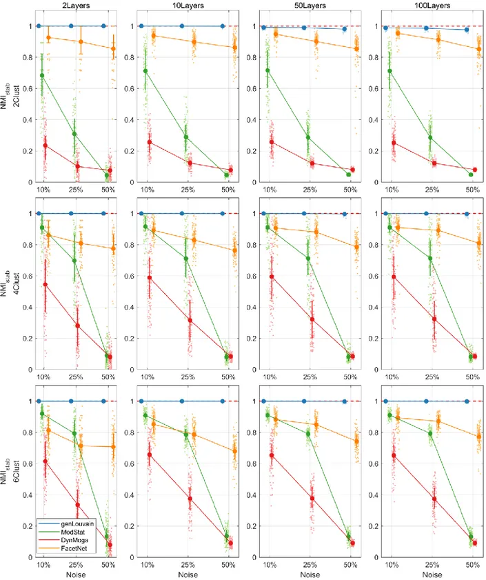
In Table 1.1 we report the results of the comparative analysis made by exploiting simulated multilayer networks with stationary community structure and graph density equal to 0.3. Analogue results have been obtained setting the graph density to the lower level, D=0.1, and can be found in the Supplementary Material, paragraph 1.6.2. In general, the results of ANOVA together with Tuckey’s post-hoc tests, show all the algorithms
28
having significantly higher performances in networks with low level of noise and high number of clusters. Overall, the figure shows genLouvain outperforming the other algorithms.
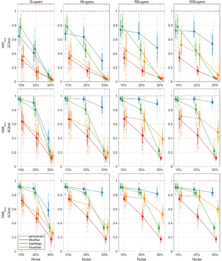
As for the accuracy (Figure 1.3) all the algorithms have performance inversely proportional to the level of noise simulated in the network. However, in noisy networks (no=50%) genLouvain and FacetNet show an improvement of the accuracy as the number of layers increases, above all if CN>2. In particular, genLouvain reaches almost the same level of accuracy in noisy and non-noisy networks, if nL≥10. On the contrary, as expected, the accuracy of ModStat is not affected by the number of layers, as it considers each slice of the network independently. Compared with the other algorithms, genLouvain displays higher level of accuracy in most combinations of Noise, Clusters Number and Number of Layers. The only exceptions are the case of low clusters number and low noise (CN=2, no=10%, nL= [2, 10, 50, 100]) in which modularity has better performances, for every value of nL.
Regarding the analysis of stability (Figure 1.4), namely the algorithms capability to recover a stable partition across the layers of the network, the algorithm with the highest performance is genLouvain for each combination of the ANOVA factors. In fact, it always
Table 1.1. Results of the ANOVA test executed for the comparative analysis on networks with stationary community structure and graph density equal to 0.3. For each considered index (dependent variables of the test) we report the degrees of freedom (dof), F and p-values relative to single factors and the interactions among them.
29
reaches the optimal value of 𝑁𝑀𝐼𝑠𝑡𝑎𝑏, despite the level of noise, number of clusters and
number of layers. On the contrary, the other algorithms are more sensitive to the ANOVA factors, especially to the level of noise and the clusters number. The algorithm ModStat
Figure 1.3. Plot of means and standard deviations of 𝑁𝑀𝐼𝑎𝑐𝑐 in the comparative analysis on networks with
stationary community structure. In the rows and the columns of the pictures we report the results for different levels of clusters number (CN) and number of layers (nL) respectively. In each subplot the 𝑁𝑀𝐼𝑎𝑐𝑐
30
has good performances, almost comparable with the genlouvain’s ones, in networks with low noise (no=10%), while FacetNet is preferable to ModStat when no≥25%.
Figure 1.4. Plot of means and standard deviations of 𝑁𝑀𝐼𝑠𝑡𝑎𝑏 in the comparative analysis on networks with
stationary community structure. In the rows and the columns of the pictures we report the results for different levels of clusters number (CN) and number of layers (nL) respectively. In each subplot the 𝑁𝑀𝐼𝑠𝑡𝑎𝑏
31
The evaluation of the global performances summarizes what observed so far. Overall genlouvain has the best performances when the aim is the detection of stationary communities. A single layer modularity approach is also appropriate in case of few layers and low percentage of noise. FacetNet shows intermediate performances, as it seems to be able to mitigate the effect of a high level of noise when it has a high number of layers to work with.
1.3.1.2. Algorithms comparison on networks with evolving community structure
In Table 2 we report the results of the comparative analysis made to test the algorithms on multilayer networks with evolving community structure, density equal to 0.3 and clusters number unchanged. We observed analogue results in networks with lower density, D=0.1, and increasing/decreasing clusters number, and we report them on the Supplementary Material, sections 1.6.1. As in the previous analysis on stationary community structure, the results of ANOVA together with Tuckey’s post-hoc tests, show all the algorithms having significantly higher performances in networks with low level of noise and high number of clusters. In reverse, the factor percentage of nodes moved (pn) does not
Table 1.2. Results of the ANOVA test executed for the comparative analysis on networks with evolving community structure and graph density equal to 0.3. For each considered index (dependent variables of the test) we report the degrees of freedom (dof), F and p-values relative to single factors and the interactions among them.
32
dramatically affect the global performances of the algorithms under analysis, meaning that the algorithms can detect small as well as big changes in community structure.
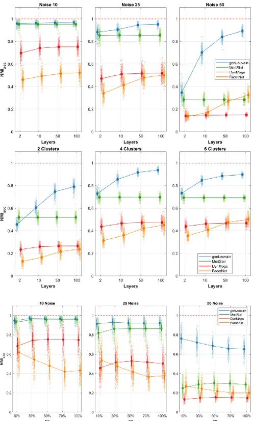
Specifically, we can unpack the results and observe the trend of each index separately. Regarding the accuracy, we show in the first row of Figure 1.5 the behavior of the algorithms with different levels of noise and number of layers. With low level of noise all the algorithms perform well, regardless of the number of layers, while as the noise increases there is a loss of accuracy. However, if nL≥10, both genLouvain and FacetNet have a significant improvement in the accuracy. In the second row is reported the effect of clusters number and number of layers on the accuracy, and it shows how the algorithms perform better when applied on networks with CN≥2, above all if nL≥10. In the third row we can observe the effect of the factors pn and no together. The percentage of nodes that change allegiance to modules does not substantially affect the accuracy of the algorithms. However, FacetNet and DynMoga show a little increase of performances when pn increases, meaning that they can easily detect big changes. Overall, genLouvain is the most accurate algorithm for each combination of the factors under analysis. The only exception is when CN=2 and nL=2, in which ModStat performs better. In general, genlouvain and ModStat have the same performances when the network has low level of noise or few layers (nL=2), while genlouvain is preferable in the other cases. FacetNet is more eligible with respect to ModStat only if the network presents a high level of noise and is composed of several layers (nL≥10).
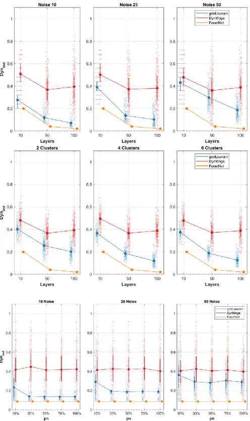
As for the evaluation of the algorithm’s dynamic (Figure 1.6) we only considered the performances of genLouvain DynMoga and FacetNet. Considering also ModStat would not be meaningful as it considers each layer independently. Moreover, we trivially considered only values of nL≥2. Also in this analysis genLouvain seem to be the most suitable algorithm as it is the fastest in identifying changes of the community structure for each combination of the factors no, nL, CN and pn. Only in the case in which CN=4 FacetNet is preferable. the factors noise and number of layers have an influence also on the rapidity of the algorithms.
33
Figure 1.5. Plot of means and standard deviations of 𝑁𝑀𝐼𝑎𝑐𝑐 in the comparative analysis on networks with
evolving community structure. In the first row we report the accuracy of the algorithms, identified with different colors, with respect to the different levels of number of layers, x-axis, and percentage of noise, columns. In the second row we show the trend of the algorithms’ accuracies with respect to the number of layers, x-axis, and clusters number, columns. In the third row we represent the accuracies mean values for each algorithm to varying of the factor pn, x-axis, and level of noise, columns.
34
Figure 1.6. Plot of means and standard deviations of 𝐷𝑦𝑛𝑖𝑛𝑑 in the comparative analysis on networks with
evolving community structure. In the first row we report the dynamic of the algorithms, identified with different colors, with respect to the different levels of number of layers, x-axis, and percentage of noise, columns. In the second row we show the trend of the algorithms’ speed with respect to the number of layers, x-axis, and clusters number, columns. In the third row we represent the 𝐷𝑦𝑛𝑖𝑛𝑑 mean values for each