High performance computing on CRESCO infrastructure: research activities and results 2015

High Performance Computing on

CRESCO infrastructure:

research activities and results 2015

Italian National Agency for New Technologies,

Energy and Sustainable Economic Development

High Performance Computing on CRESCO Infrastructure:

research activity and results 2015

Contributions provided by a selection of users of the CRESCO infrastructure Scientific

Editor: Giovanni Ponti, ENEA, DTE-ICT-HPC, Research Centre Portici

Acknowledgements: We wish to thank Gianclaudio Ferro for providing the Reporter system

(http://hdl.handle.net/10840/5791) to collect contributions and to build the Volume

Cover: Amedeo Trolese, ENEA, DTE-ICT-PRA, Research Centre Frascati

ISBN: 978-88-8286-342-5

Contents

Foreword

5

Ab Initio Carr-Parrinello Simulations of High Temperature GeO2: a comparison of the

effects of plane waves cut-off and time step choice

G. Mancini, M. Celino

6

Effects of preferential diffusion on turbulent lean premixed CH4/H2 - Air slot flames

D. Cecere, E. Giacomazzi, N.M. Arcidiacono, F.R. Picchia

10

A homemade Fortran code to analyse results from CPMD Calculations

E. Burresi, M. Celino

16

Inter-layer synchronization in multiplex networks

I. Sendiña-Nadal, I. Leyva, R. Sevilla-Escoboza, R. Gutiérrez, J.M. Buldú, J.A.

Almendral, S. Boccaletti

21

Atmospheric Pollution Trends simulated at European Scale in the framework of the

EURODELTA 3 Project

G. Briganti, A. Cappelletti, M. Mircea, M. Adani, M. D'Isidoro

26

MCNP simulations supporting PWR GEN-II and III safety studies and feasibility study of

minor actinides irradiation in the Tapiro research reactor

P. Console Camprini, K. W. Burn

31

Monte Carlo study of dose-area-product properties in radiatherapy photon beams with

small field sizes

Claudio Caporali

35

Simulations of linear and nonlinear interactions between alfven modes and energetic

particles

S. Briguglio, G. Fogaccia, V. Fusco, M. Martone, G. Vlad, X. Wang, T. Wang

39

Analysis of the wave field in front of the U-OWC

P. Filianoti, L. Gurnari

48

A novel charge-equilibration method for self assembly of organics on metal surface

A. Palma, M. Satta, S. Tosti

52

Enlightening of water self-assembling phenomena onto the (101) TiO2 anatase surface by

atomistic multi-scale modeling

Enlightening of water self-assembling phenomena onto the (101) TiO2 anatase surface by

atomistic multi-scale modeling

F. Gala, L. Agosta, G. Zollo

56

Implementation of an air quality forecast system over Italy

M. Adani, M. D'Isidoro, G. Briganti, A. Cappelletti

63

First-principles investigation of the amino acids adsorption to hydrated non-polar ZnO

surface

F. Buonocore, C. Arcangeli, M. Celino, F. Gala, G. Zollo

68

Performance analysis of CRESCO clusters by using DGEMM subroutine

Simone Giusepponi

74

CFD Simulations of hydrocarbons reforming with CO2 capture in a fluidised bed

carbonator

A. Di Nardo, S. Stendardo, G. Calchetti

80

CP2K performance on CRESCO4 HPC system

M. Gusso

84

Ab-initio study of silicon based materials for photovoltaic applications

S. Giusepponi, M. Gusso, M. Celino, U. Aeberhard, P. Czaja

88

Quantum Espresso performance on ENEA and JSC HPC infrastructures

S. Giusepponi, M. Gusso, M. Celino, U. Aeberhard, P. Czaja

93

Electronic band structure, lattice dynamics, and related superconducting properties of

niobium from first–principles calculations

G. De Marzi

99

Language discrimination via a neural network approach

A. Mariano

105

Web Crawling tool integration in ENEAGRID

G. Santomauro, G. Ponti, F. Ambrosino, G. Bracco, A. Colavincenzo, A. Funel, G.

Guarnieri, S. Migliori, M. De Rosa, D. Giammattei

110

Fast switching alchemical simulations: a non equilibrium approach for drug discovery

projects on parallel platforms

P. Procacci

115

Simulation of photon beams for radiotherapy application

Simulation of photon beams for radiotherapy application

L. Silvi, M. Pimpinella

124

Transport study of Neon impurity seeded FTU plasma by Gyrokinetic simulations

V. Dolci, C. Mazzotta, FTU team

129

Self-Assembly of Triton X100 in Water Solutions: A Multiscale Simulation Study Linking

Mesoscale to Atomistic Models

A. De Nicola, Z. Ying, M. Celino, M. Rocco, T. Kawakatsu, G. Milano

135

Computer Simulation of Triglycerides

A. Pizzirusso, Y. Zhao, A. De Nicola, G. Milano

141

Biconnectivity of Very Large Social Graphs

G. Chiapparo, U. Ferraro Petrillo, D. Firmani, L. Laura

144

Do emission policies reduce ozone risk to European forests?

A. Anav, A. De Marco

148

Multidecadal hindcast of the mediterranean thermohaline circulation

G. Sannino, A. Carillo, M.V. Struglia

151

The core design of Gen-IV Lead Fast Reactors using the ERANOS code on the CRESCO

HPC infrastructure

M. Sarotto, G. Grasso, F. Lodi

155

Surface functionalization of ZnO for solar energy conversion devices: new insights from a

first-principles study

A.M. Rodríguez, A.B. Muñoz-García, C. De Rosa, M. Pavone

159

Car-Parrinello molecular dynamics of liquid NaNO3

R. Grena, M. Celino

164

First-principle determination of equilibrium and out of equilibrium excited state

properties of surfaces and 2D materials

M. Marsili, O. Pulci, M.S. Prete, A. Mosca Conte, P. Gori

168

Study of the Zr Doping in the Cerium Oxide through First-Principles Calculations

F. Rizzo, G. De Marzi

174

The influence of TiO2 and Ti dopants on the hydrogen mobility through MgH2-Mg

interface

The phase structure of the Naming Game in the stochastic block model

F. Palombi, S. Toti

182

Transcriptome assembly of C. sativus

A. Conte, G. Aprea, M. Pietrella

187

Analysis of current fast neutron-flux monitoring instrumentation targeted for the DEMO

LFR ALFRED

L. Lepore, R. Remetti, M. Cappelli

192

Analysis of the chaotic behavior of the Lower Hybrid Wave propagation in magnetised

plasma by Hamiltonian theory

A. Cardinali, A. Casolari

198

Bi(111) nanofilms: quantum confinement and surface states

G. Cantele, D. Ninno

202

Multiphase rotating turbulent flows in gas turbine internal cooling channel

D. Borello, F. Rispoli, A. Salvagni, P. Venturini

206

CRESCO numerical combustion analysis of swirling micro-meso combustion chambers

A. Minotti

210

CFD modeling of a flameless furnace: comparative evaluation of turbulent combustion

models with two software on a HPC platforms

C. Mongiello, G. Guarnieri, G. Continillo, D. Iorio, G. Maio, F.S. Marra

214

Role of the sub-surfece vacancyu in the amino-acids adsorption on the (101) anatase TiO2

surface: a first principles study

L. Maggi, F. Gala, G. Zollo

220

Neutronics calculations for the design of DEMO WCLL reactor

R. Villari, G. Mariano, A. Del Nevo, D. Flammini, F. Moro

227

The network architecture underlying the CRESCO infrastructure of ENEA Portici

Foreward

During the year 2015, CRESCO high performance computing clusters have provided more than 46

million hours of “core” computing time, at a high availability rate, to more than one hundred users,

supporting ENEA research and development activities in many relevant scientific and technological

domains. In the framework of joint programs with ENEA researchers and technologists, computational

services have been provided also to academic and industrial communities.

This report, the seventh of a series started in 2008, is a collection of 46 papers illustrating the main

results obtained during 2015 using CRESCO HPC facilities. We registered an important increase on

contributions this year, testifying the importance of the interest for HPC facilities in ENEA research

community. The topics cover various fields of research, such as material science, efficient combustion,

climate research, nuclear technology, plasma physics, biotechnology, aerospace, complex systems

physics. The report shows the wide spectrum of applications of high performance computing, which

has become an all-round enabling technology for science and engineering.

Since 2008, the main ENEA computational resources is located near Naples, in Portici Research

Centre. This is a result of the CRESCO Project (Computational Centre for Research on Complex

Systems), co-funded, in the framework of the 2001-2006 European Regional Development Funds

Program, by the Italian Ministry of Education, University and Research (MIUR).

The Project CRESCO provided the resources to set up the first HPC x86_64 Linux cluster in ENEA,

achieving a computing power relevant on Italian national scale (it ranked 126 in the HPC Top 500 June

2008 world list, with 17.1 TFlops and 2504 cpu cores). It was later decided to keep CRESCO as the

signature name for all the Linux clusters in the ENEAGRID infrastructure, which integrates all ENEA

scientific computing systems, and is currently distributed in six Italian sites.

In 2015 the ENEAGRID computational resources attained the level of about 8000 computing cores (in

production) and a raw data storage of about 900 TB. Those values have been reached thanks to the

availability of the new cluster CRESCO5 (640 cores Intel, 16.4 Tflops, QDR Infiniband network), in

addition to the CRESCO3, and CRESCO4 clusters.

The success and the quality of the results produced by CRESCO stress the role that HPC facilities can

play in supporting science and technology for all ENEA activities, national and international

collaborations, and the ongoing renewal of the infrastructure provides the basis for an upkeep of this

role in the forthcoming years.

In this context, 2015 is also marked by the signature of an agreement between ENEA and CINECA, the

main HPC institution in Italy, to promote joint activities and projects. In this framework, CINECA and

ENEA participated successfully to a selection launched by EUROfusion, the European Consortium for

the Development of Fusion Energy, for the procurement of a several PFlops HPC system, beating the

competition of 7 other institutions. The new system MARCONI-FUSION started operation in July

2016. The ENEA-CINECA agreement is a promising basis for the future development of ENEA HPC

resources in the coming years.

Dipartimento Tecnologie Energetiche,

Divisione per lo Sviluppo Sistemi per l'Informatica e l'ICT

CRESCO Team

Ab Initio Carr-Parrinello Simulations of High Temperature

GeO

: a comparison of the effects of plane waves cut-off and

time step choice.

Giorgio Mancini

_{and Massimo Celino}

Università di Camerino, sezione di Fisica della Scuola di Scienze e Tecnologie, Via Madonna delle Carceri 62032, Camerino (MC), Italy

2_{ENEA, Ente per le Nuove Tecnologie, l’Energia e lo Sviluppo Economico Sostenibile}

C. R. Casaccia, Via Anguillarese 301, 00123 Roma, Italy

ABSTRACT. Ab initio Carr-Parrinello simulations of high temperature GeO

have been carried out using a

set of different parameters supposedly significantly affecting the results, as well as the computing times. A

particular attention has been paid to the effects related with the plane waves cut-off using lower and higher

values than commonly suggested. Comparisons of the results for the different values are presented and

illustrated indicating that the results are essentially the same.

1 Introduction

We have recently presented the preliminary results of the simulations of a 240 atoms, high

temper-ature GeO

system, entirely carried out by ab initio (AI) molecular dinamics (MD) simulations

us-ing the CPMD (Carr-Parrinello Molecular Dynamics) software [1]: an approach distinct from the

ones consisting in using classical molecular dynamics (CMD) results for GeO

at much higher

tem-peratures (4000-7000K) as starting configurations for AI simulations to be carried out at lower final

temperatures [2]. The main reason to adopt such a hybrid approach is that it allows to bypass both

the limitations due to the short time scale accessible from ab initio simulations and the usually long,

delicate, often unsuccessful process needed to prepare a “stable” system to start with (CPMD

simu-lations on unstable systems abruptly diverge even from the very first runs at temperatures as low as

10

_~50K).

As for the computation times required by ab initio simulations, once the general frame in which

they are carried out is set (let's simplistic say, once functionals and pseudo-potentials are chosen),

they only depend on the values used for both the time step and the kinetic energy cut-off for

elec-tronic plane waves expansion: they must respectively be taken to be short and high enough to allow

for meaningful, correct simulations; but shorter time steps and higher cut-offs mean longer

compu-tational times and/or larger compucompu-tational resources.

In the results we have previously presented for GeO

[3], strictly abiding by the prescriptions given

in the CPMD user's manual for such a choice [4],

we have used

a time step of 5 a.u (

_{~0.121 fs) and}

a value of 60 Ry for the p

lane waves cut-off: respectively a higher and a lower value than the ones

commonly suggested and used in literature (3 a.u. and 70-75 Ry) [1, 5].

To evaluate the extent of the possible differences on the results as a consequence of a more

demand-ing choice of such parameters, we have carried out two additional CPMD simulations series to

ob-tain high temperature GeO

using higher cut-offs values (80 and 90 Ry) on the same initial system

we previously studied.

2 Computational resources

The calculations have been performed by using the facilities and services available at the ENEA

GRID infrastructure (Italy). Molecular Dynamics simulations have been carried out using CPMD

v3.15.1 on CRESCO4 cluster, using 512 processors per run, 400 GB of disk storage has been

gran-ted on the PFS/porq1_1M file system.

3 Computational details

We have performed three separated series of Carr-Parrinello, first-principles simulations on a GeO

system consisting of 240 atoms; the series correspond to kinetic energy cut-off values for plane

waves expansion of 60, 80 and 90 Ry, respectively.

The initial GeO

configuration to start the

simu-lations on has been generated placing 80 germanium and 160 oxygen atoms at random in a cubic

simulation box of linear dimensions L=15.602 angstroms, corresponding to a density ρ = 3.66

gr/cm

_{; the only condition imposed has been their distances being larger than certain suitable values}

[3].

To perform CPMD simulations, we have adopted the generalized gradient approximation (GGA) for

the exchange and correlation part of the total energy and norm conserving pseudo-potentials with

the BLYP exchange–correlation functional using the Troullier–Martins parametrization for the

core-valence interactions.

We have run the wave-function optimization processes imposing that the wave-functions be

con-verged very well by setting a very strict convergence criterion (GEMAX < 10

_{) [4]. The}

sub-sequent geometry optimizations too have been performed setting a stricter convergence criterion

than usual (GNMAX < 10

_{) [4]. An integration time step of 3 a.u. (0.072fs) has been used for the}

initial optimizations. After wave function and geometry optimizations, Carr-Parrinello molecular

dynamics simulations have been carried out on the systems heated up and equilibrated at 10K, 50K,

100K,150K, 200K, respectively, and up to 3000K by steps of 100K.

To allow for shorter equilibration times, “massive” thermostatting has been used for the ions (a

Nosé-Hoover chain thermostat placed on each ionic degree of freedom). A second Nosé-Hoover

chain thermostat has been set on the electronic degrees of freedom to keep electrons on the

Born-Oppenheimer surface throughout all MD simulations. Characteristic thermostats frequency of 1000

cm

_{for ions and 10000 cm}

_{for electrons have been used. The default value of 400 a.u. has been}

used for the fictitious electronic mass.

The integration time step of 5 a.u. (0.12fs) used on the entire temperature range for the 60 Ry

cut-off have turn out to be too long for the higher cut-cut-offs since the very beginning (the simulations at

5K have diverged after a few steps). We are not able to tell whether this is a generalized behaviour

or not, but we systematically have experienced it on several configurations. Consequently a time

step of 3 a.u. has been used for the 80 and 90 Ry (this turned out to be the longest possible time step

at all temperatures for us to have stable simulations).

On a computer equipped with SD hard disks, 64 GB ram (much larger than effectively used) and a

last generation Intel I7 on which CPMD runs on twelve almost perfectly balanced parallel threads,

the required time per single step of CPMD has dramatically grown when switched from 60 Ry to 80

or 90 Ry. On the contrary, when run on CRESCO4 cluster batch queues, 512 cpu's have proved

suf-ficient to obtain the same computation times per single CPMD step for all the cut-offs values. As a

matter of facts, on the I7, the required times for 80 and 90 Ry where practically the same and

ap-proximately three times those for 60 Ry; on the other hand, the simulations for 60 and 90 Ry have

run about ten and thirty times faster on CRESCO4 than on I7. In conclusion, the simulation

pro-cesses times have depended only on the time step; the higher cut-offs requiring a time almost twice

longer than for 60 Ry: a ratio not to neglect when it comes to ab initio simulations.

4 Results and conclusions.

It is important to notice how the geometry optimization processes have determined different initial

positions for the three systems, so that they have undergone independent, separate evolutions in

time and temperature from the very beginning. Since the simulations have begun at different times,

we have compared them in the common time interval they have covered: a total time of 36 ps, 16 ps

of which spent at 3000K.

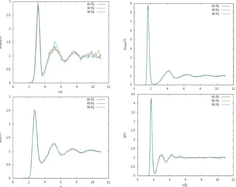
The results of the simulations are depicted in figs. 1-3, showing radial distribution and static

struc-ture functions. Similar, almost superposing, results hold for dn(r), angles and bonds distributions.

Fig. 1: Partial and total radial distribution functions for cut-offs 60, 80 and 90 Ry.

The simulations have essentially led to the same results for all relevant properties, thus validating

the choice of using lower wave-function expansions cut-off for shorter simulations times to get the

maximum possible efficiency while maintaining accuracy.

Fig. 2: Partial and total static structure functions for cut-offs 60, 80 and 90 Ry.

References

[1] CPMD, Copyright IBM Corp 1990-2008, Copyright MPI für Festkörperforschung Stuttgart 1997-2001.

[2] M. Hawlitzky, J. Horbach, S. Ispas, M. Krack, and K. Binder. “Comparative classical and ab initio

mo-lecular dynamics study of molten and glassy germanium dioxide”. J. Phys. Condens. Matter 20 (2008)

285106 (15pp)

[3] G Mancini, M. Celino, and A. Di Cicco. “Ab-Initio Molecular Dynamics Simulation of High Temperature

GeO

”. High Performance Computing on CRESCO infrastructure: research activities and results 2014,

ISBN: 978-88-8286-325-8 (2015) pp. 46-49.

[4] The CPMD Consortium. “Car-Parrinello Molecular Dynamics: An ab initio Electronic Structure and

Molecular Dynamics Program. Manual for CPMD, version 3.15.1”.

[5] Peter Broqvist, Jan Felix Binder, Alfredo Pasquarello. “Atomistic model structure of the Ge(100)–GeO

Effects of preferential diffusion on turbulent

lean premixed

CH

₄

_/H

₂

_{− Air slot flames}

D. Cecere

, E. Giacomazzi

, N.M. Arcidiacono

and F.R. Picchia

❆❜str❛❝t✳ Nowadays, in the context of CO2 reduction and gas turbine fuel

flex-ibility, the interest in acquiring know-how on lean Hydrogen Enriched Natural Gas (HENG) is growing. This article provides a detailed analysis of a turbulent (Rejet = 2476, Ret = 236) lean (Φ = 0.7) CH4/H2 −air premixed slot flames

(unconfined and at atmospheric pressure) highlighting the effects of two differ-ent hydrogen contdiffer-ents in the inlet mixture (20% and 50% by volume). The data were generated and collected setting up a three-dimensional numerical experiment performed through the Direct Numerical Simulation (DNS) approach and using high-performance computing. Finite difference schemes were adopted to solve the compressible Navier-Stokes equations in space (compact sixth-order in staggered formulation) and time (third-order Runge-Kutta). Accurate molecular transport properties and the Soret effect were also taken into account. A detailed skele-tal chemical mechanism for methane-air combustion, consisting of 17 transported species and 73 elementary reactions, was used. The analysis reports average and rms fluctuation of velocity components, temperature and main chemical species mass fractions. New scientific insight is delivered by analysing the probability density functions of several quantities: curvature, shape factor, alignment between vorticity vector and flame surface normal, displacement speed and its components. Correlations between the flame thickness and the progress variable and curvature are also investigated, as well as correlation between strain rates and curvature, and equivalence ratio and curvature. An expression of displacement speed, with dif-fusion terms taking into account differential difdif-fusion of progress variable species components is derived. The effect of thermal diffusion is also considered. The effects of differential diffusion of several species on the local equivalence ratio are quantified: the maximum variation from the nominal inlet value is ∼ 9% and it is due to H2 and O2. The addition of Hydrogen reduces the displacement speed at

negative curvatures in a range that depends on the local progress variable value, with a maximum variation of −33% between the two flames. The database will also be helpful to validate subgrid models for Large Eddy Simulation.

1

Test case definition

The test case defined for this study consists in an unconfined premixed slot-burner flame at atmospheric pressure. A slot-burner Bunsen configuration is especially interesting due to the presence of a mean shear in the flow. The configuration is similar to that of the experimental device already analysed in [1] but with smaller dimensions (h = 1.2mm vs 25.4mm of slot width in the experimental setup) and higher bulk velocities (100m/s) compared to experiment (3 to 12m/s) to artificially decrease the hydrodynamic DNS times. It consists of a central slot-jet of premixed reactants surrounded on both longer sides by two

Case Φ nH₂ Tu Tb SnSL δnSL SSL δSL δSD

A 0.7 0.2 600 2072 1.03 0.368 1.01 0.378 0.1329 B 0.7 0.5 588 2084 1.37 0.314 1.34 0.315 0.1096

Table 1: CH4/H2−Air laminar flames characteristics (A-B) based on the 17-species chemical mechanism

adopted in the present DNS [5]. The number of Hydrogen moles nH₂ is defined as nH₂ = xH₂/(xH₂+

xCH₄). The superscripts nS and S in the laminar flame speed and flame front thickness, respectively

stand for “no Soret” and “Soret” effect not included and included in the laminar flame calculation. Units: [K] for temperature, [m/s] for flame speed, [mm] for flame front thickness.

Jets A (B) U0,in Tin u′in δcorrz,in LDuct h

Central 100 (100) 600 (588.5) 12 (12) 0.4 4 1.2

Surrounding 25 (25) 2072 (2084) 0.01 (0.01) 0.1 - -Table 2: Boundary conditions imposed at the inlet of the three channels. In particular, u′

z= u ′ x= u ′ yand δcorr

z,in, δx,incorr= δy,incorr= δz,incorr/2 are used as input to the Klein procedure to produce synthetic turbulence

at the inlet of the three channels. Units: [m/s] for velocity, [K] for temperature, [mm] for turbulent correlation length scale, duct length, LDuct, and its width, h.

coflowing jets. The central slot-duct is 1.2 mm wide (h) and 4 mm long; its two walls have a thickness hw= 0.18 mm and are assumed adiabatic in the simulation.

The central jet is a lean (equivalence ratio Φ = 0.7) mixture of methane, hydrogen and air with fuel molar fractional distribution of 20% H2 and 80% CH4 for the flame A, and of 50% H2 and 50% CH4

for the flame B. Mixture temperature is 600 K for flame A, and 588 K form flame B: the latter lower temperature was chosen to achieve the same kinematic viscosity and Reynolds number for the central reactive jet in the two simulations. The surrounding jets have the composition and temperature of the combustion products of the laminar freely propagating flame associated to the central jet mixture. The unstrained laminar flame properties at these conditions computed using Chemkin [2] are summarized in Table 1. In this table, Φ represents the multicomponent equivalence ratio of the reactant jet mixture, Φ = [(XH₂+ XCH₄)/XO₂]/[(XH₂+ XCH₄)/XO₂]stoich, Tu is the unburnt gas temperature, Tb the burnt

gas temperature, SL represents the unstrained laminar flame speed and δth= (Tb− Tu)/|∂T/∂x|max is

the flame front thermal thickness based on the maximum temperature gradient.

The central jet has a velocity of 100 m/s (imposed as a mean plug-flow at the inlet of the 4 mm long central duct). Homogeneous isotropic turbulence is artificially generated at the inlet of the central duct by forcing a turbulent spatial correlation scale in the streamwise direction δcorr

z,in = 0.4 mm and a

streamwise velocity fluctuation u′

z = 12 m/s used as inputs to the Klein’s procedure [3] (see Table 2).

The surrounding flows have a velocity of 25 m/s (imposed as a mean plug-flow) and no turbulence is forced. The actual jet Reynolds number based on the centerline streamwise velocity peak at the central duct exit and its width h is Rejet= Uoh/ν = 2476. Other parameters characterizing the present lean

premixed turbulent flame are reported in Table 3. These parameters locate the present flames in the Thin Reaction Zone of the combustion diagram.

The computational domain is composed of four structured blocks and its characteristics are summarized in Table 4. The domain size in the streamwise (z), crosswise (y) and spanwise (x) directions is Lx×

Ly× Lz = 24h × 15h × 2.5h, h being the slot width (h = 1.2 mm). The grid is uniform only in the

x spanwise direction (∆x = 20 µm), it is refined in the y and z direction near the inlet duct walls and coarsened (up to ∆y ∼ 250 µm) only in the y direction far from the central jet at the surrounding (y > 0.015 m) where non reflecting boundary conditions are applied and fluctuations are small. The domain is almost identical and the resolution is the same of the work of Richardson et al. [4] and Sankaran et al. [5]. The DNS was run at atmospheric pressure using a 17 species and 73 elementary

Jet exit velocity peak, U0 [m s−1] 110

Jet exit velocity fluctuation, u′_{[m s}−1_{] 12}

Jet exit turbulent length scale, Lt [mm] 1.05

Jet Reynolds number, Rejet= U0h/ν 2476

Turbulent Reynolds number, Ret= u′Lt/ν 236

Kolmogorov lenght scale, ηK[µm] 17.42

Turbulent/chemical speed ratio, u′

/SL 11.88 (8.95)

Turbulent/chemical length scale ratio, Lt/δL 2.78 (3.22)

Damkohler number, SLLt/u′δL 0.238 (0.371)

Karlovitz number, (δL/ηK)2 471 (329)

Table 3: Actual turbulent combustion parameters characterizing the simulated CH4/H2 − Air lean

premixed flames (flame B in parentheses). The turbulent velocity fluctuation and the integral length scale were evaluated at the center of the exit of the central slot-duct. The laminar flame speed and the flame front thickness including the Soret effect were assumed as combustion parameters. The kinematic viscosity used in the calculation of the central jet Reynolds number is that of the inlet CH4− H2/Air A

mixture, ν = 5.327 · 10−5_m2_s−1_{. It is observed that sometimes the Karlovitz number is estimated using}

the diffusive thickness: with this definition Ka = 58 for flame A, and Ka = 40 for flame B. Domain size (Lx×Ly×Lz) 24h × 15h × 2.5h

Nx×Ny×Nz 1550 × 640 × 140

Minimum grid space 9 µm

Table 4: Characteristics of the computational domain. Note that Lx, Ly and Lz refer to the spanwise,

crosswise and streamwise directions, respectively.

reactions kinetic mechanism [5]. Periodic boundary conditions were applied in the crosswise direction, while improved staggered non-reflecting inflow and outflow boundary conditions (NSCBC) were adopted at the edges of the computational domain in the y and z directions [6, 7].

The simulation was performed on the linux cluster CRESCO (Computational Center for Complex Sys-tems) at ENEA requiring 1.5 million CPU-hours running for 20 days on 3500 processors. The solution was advanced at a constant time step of 2.3 ns; after the flame reached statistical stationarity, the data were collected through 4 τU, τU = 0.218 ms being the flow through time based on the jet exit duct

centerline velocity and the total streamwise domain lenght.

2

Results and discussion

In order to investigate the effect on local mixture equivalence ratio of differential and thermal diffusion associated with light species as H2and H, the local equivalence ratio Φ, is shown for both flames in Fig.

1 as a function of the normalized curvature at different values of the progress variable. The results are obtained from two DNS in which the diffusion term Jn is calculated with only the first term and the

complete expression of Eq. (1), respectively. Jn= −ρ Wn Wmix Dn∇Xn− ρYnDTn ∇T T , (1)

The equivalence ratio Φ is positively correlated with curvature at all progress variable iso-surfaces; the strongest variation is seen in the reaction zone (c ∼ 0.7). This positive correlation can be explained by considering that H2 and H are preferentially focused into areas with positive curvature and defocused

Figure 1: Equivalence ratio at different levels of the progress variable c as a function of the normalized curvature: (#) c = 0.7, (3) c = 0.6, (2) c = 0.4, (Dash dot dot line) nominal flame equivalence ratio Φ. (a) Flame A: (solid line) without Soret effect, (dashed line) with Soret effect. (b) Flame A and B with Soret effect: (solid line) flame A, (dashed line) flame B.

positive correlation with curvature since it promotes diffusion of light molecules towards high temper-ature regions. In fact, the maximum equivalence ratio variation is ∼ 3.7% for flame A and ∼ 9% for flame B when thermal diffusion effects are considered in the simulation (∼ 2.6% for flame A when only differential diffusion effect is considered).

The local enrichment of the flame at positive curvatures is also shown in Fig. 2 for the flame A, where the instantaneous flame surface (c ∼ 0.72) coloured by the normalized mean curvature ∇ · n δL, is shown

together with two instantaneous iso-surfaces of the equivalence ratio (Φ = 0.657 and 0.757). While in the laminar flame, the effect of the differential diffusion is only a reduction of the equivalence ratio towards leaner condition, in the 3D DNS, the effect of positive curvature (e.g., see the progress variable isosurface at c = 0.72 coloured in yellow in Fig. 2) produces also local enrichment of the flame (e.g., see the orange Φ grid surface in Fig. 2).

In order to quantify differential diffusion effects in the two flames, the general method of Sutherland [9, 8] is adopted, and the contribution of major species (H2, O2, H, CH4) differential diffusion term ki to

the local variation of mixture fraction, is calculated as: ki= ∇ · jic, j c i = γiWi∇ · [ ρ WMix (Di− D)∇Xi] (2)

where γi =P_e∈Neδeαe,i, δe are the elemental mass fraction weights of Bilgers’s mixture fraction, Ne

the number of element e defining the mixture fraction, αe,i is the number of atoms of element e in

species i, D the diffusivity of the mixture fraction [8], Di the species mass diffusivity.

Figures 3a-b show the species mixture fraction source terms, as a function of curvature within the flame brush for both flames at two progress variable values. At the leading edge, the largest contribution to the decrease of the mixture fraction at negative curvatures, is due to the kO₂ and kH₂, that for flame B

(that presents a greater decrease of equivalence ratio with respect to flame A for negative curvatures, see Fig.1b) are both negative. For positive curvatures, and for both flames, the positive value of kO2f or∇ · δL> 1 is counteracted by the negative value of kH2. This reduces the increase of equivalence

ratio since kHis negative and kCH₄is negligible for positive curvatures. At the trailing edge of the flame

(see circles in Fig.1b), the increase of the equivalence ratio is observed for ∇ · δL > −2, (∇ · δL > −1)

Figure 2: Instantaneous snapshot of the progress variable iso-surface at c = 0.72 coloured with nor-malized curvature ∇ · nδL and two iso-surfaces of equivalence ratio at φ = 0.657 (blue) and φ = 0.757

(orange), respectively, for the flame A.

Figure 3: Species differential diffusion source index kiat two level of the progress variable c as a function

of the normalized curvature (a,b) and normalized strain (c,d) for flame A (solid line) and B (dashed line).

the same order for both flames for positive curvatures. In the enriched flame, the kH₂ term presents

a strongly positive correlation with curvature, and despite the bigger counteracting effect of kH, it is

responsible for the bigger increase of equivalence ratio at positive curvatures of flame B.

Figures 3c-d show the species differential diffusion coefficient as a function of tangential strain rate. The source term related to CH4 (with Le ∼ 1) has no correlation with strain. At the leading edge, flame

A is weakly affected by tangential strain, the kO₂, kH₂ are negative, but counteracted by the positive

value of kH. In flame B the kH₂ has a negative correlation with strain; despite the positive correlation

of kH, the net effect is a decrease of the equivalence ratio. At the trailing edge, there is an increase of

the equivalence ratio that has a positive correlation with the module of the strain for both flames (with a greater correlation for flame B). The kH₂ term is always positive for both flames; while for flame A

is approximately constant, it has a stronger positive correlation with the module of strain in flame B. For flame A, the equivalence ratio is approximately constant for compressive strains, since the negative kH counteracts the positive value of kO2. For positive strain, the equivalence ratio trend follows that

of kO2. The greater correlation of equivalence ratio of flame B (that for positive strain has a thinner

structure than flame A) is completely related to kH₂ and kO₂ trends.

References

[1] S.A. Filatyev, J.F. Driscoll, C.D. Carter, J.M. Donbar, Measured properties of turbulent premixed Flames for model assessment, including burning velocities, stretch rates, and surface densities, Combust. Flame 141, 1-21, 2005.

[2] R.J. Kee, G. Dixon-Lewis, J. Warnatz, M.E. Coltrin, Miller JA, Moffat HK, The CHEMKIN Collection III: Transport, San Diego, Reaction Design, (1998).

[3] M. Klein, A. Sadiki, J. Janicka, A digital filter based generation of inflow data for spatially developing direct numerical or large eddy simulations, J. Comput. Phys. 186, (2003), 652-665. [4] E.S. Richardson, R. Sankaranb, R.W. Grout, J.H. Chen, Numerical analysis of reaction-diffusion

effects on species mixing rates in turbulent premixed methane-air combustion, Combust. Flame 157 (2012) 506-515.

[5] R. Sankaran, E.R. Hawkes, J.H. Chen, T. Lu, C.K. Law, Structure of a spatially developing turbulent lean methane-air Bunsen flame, Proc. Combust. Inst., 31, (2007) 1291-1298.

[6] T.J. Poinsot, S.K. Lele: Boundary Conditions for Direct Simulations of Compressible Viscous Flow. J. Comput. Phys., 101:104-129 (1992).

[7] J.C. Sutherland , C.A. Kennedy , Improved boundary conditions for viscous, reacting, compressible Flows, J. Comput. Phys., 191:502-524, 2003.

[8] Fabrizio Bisetti, J.-Y. Chen, Jacqueline H. Chen, Evatt R. Hawkes, Differential diffusion effects during the ignition of a thermally stratied premixed hydrogen-air mixture subject to turbulence, Proc. Combust. Inst. 32 (2009) 1465-1472.

[9] J.C. Sutherland, P.J. Smith, J.H. Chen, Quantification of differential diffusion in non premixed systems, Combust. Theory Model. 9, (2005) 365-383.

A HOMEMADE FORTRAN CODE TO ANALYSE

RESULTS FROM CPMD CALCULATIONS

E. Burresi

, M. Celino

ENEA, SSPT Department, PROMAS Division, MATAS Laboratory, C.R. Brindisi 2_{ENEA, DTE Department, ICT Division, C.R. Casaccia, Rome}

ABSTRACT.

In order to analyse the ab-initio molecular dynamics trajectories computed by the

CPMD (Car-Parrinello Molecular Dynamics) code, we needed to build a customized software

package, named QDprop, which is able to manage efficiently its large data outputs. The software

package is used to detect the interesting chemical and physical processes happening during the

atomic scale dynamics of the system and to calculate the associate structural and electronic

properties. The materials which were characterized are quantum dots with spherical and prismatic

shape. This software is written in Fortran language and actually does not work in parallel mode. The

software has been tested on CdS nanostructures (for quantum dots applications) to analyse their

chemical behaviour in the range of temperatures used in the experimental laboratories. Indeed

during their production, the temperature can modify their atomic scale structures and thus their

chemical and optical properties. Since this modifications are difficult to measure experimentally

during the production phase a modeling approach is needed in order to optimize the at the nanoscale

the final chemical and physical properties

1 A Fortran code to analyse the dynamic of nanoclusters

A preliminary version of the code was used to analyse structural properties of single wurtizte CdS

quantum dots [1], by correlating these properties to the electronic behaviour [2]; the code was

named QDprop. Recently, a new version of this code has been realized and employed to analyse a

CdS nanocluster with prismatic shape. Actually, the code works only for two classes of atoms,

typically chalcogens and metals, considering also the different symmetries.

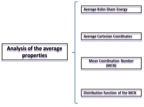
A brief scheme of the algorithm as it is built is reported in Figure 1.

Fig 1:

General overview of QDprop

The initial part of the code is dedicated to the static allocation of the memory, declaration of the

variables and definition of the input data. The CPMD trajectory is stored in a file named

TRAJECTORY (or TRAJ.xyz) where each configuration is written after some number of step

(controlled in CPMD input); so that the dimension of this large matrix is an input of the program.

The most important input parameters are:

-

Size of the matrix of the trajectory (integer)

-

Number di atoms specie 1 and number of atoms specie 2 (integer)

-

Number of step of the dynamics (integer)

-

Atomic number of the atoms (integer)

-

Atomic mass of the atoms (real)

-

Logical variable to print the results (integer)

-

Restart variable which defines the point where the algorithm starts to analyse the trajectory

(integer)

-

Number of configuration used to calculate the averages (integer)

-

Core radius which defines the core and surface layer (real)

In addition, before of the subroutine dedicated to the calculation, a little subroutine is called in order

to check the memory addresses. After these primary steps, we show the core of the algorithm in

Figure 2.

Fig 2:

Flowchart of QDprop

For analysing the trajectory a cycle do-loop is executed over the number of steps of the trajectory;

for each step of the trajectory, in order to count the number of atoms nearest neighbours, the cutoff

of the distance Cd-S is determined. In addition, in order to define the superficial layers the radial

distance between each atoms and the center of mass is calculated; if the radial distance is greater

than core radius then the atom belongs to the superficial layer. Once we defined the atoms for the

surface and for atoms of the core, RDF and MSD were obtained both for core and surface and for

the whole cluster. The last section of this algorithm regards the calculation of the average

properties. The code allows to set the number of the configurations for calculating the averages; this

parameters is an input variable. In Figure 3 we report the average quantities obtained by using this

code.

The main physical quantites obtained from the code are printed in files ASCII and available for data

analysis using software like OriginLAB or Excel.

Regarding the electronic properties, the code performs the calculatuion of the total and partial

density of the electronic states, as well as the inverse participation ratio IPR function. Actually the

electronic and the structure properties are calculated separately and the routine for electronic

properties will be implemented into QDprop as soon as possible.

2 Application

Previous versions of this code were used to study the dynamics of nanocluster from CPMD data; for

example in [1] and [2] as well as in the last CRESCO reports [3,4]. Generally, on the CRESCO

platform the average time to perform the analysis of a single step of the trajectory is around 10

seconds. Generally , trajectories are very large because several picoseconds of dynamics are stored

during the quantum simulation. The main critical issue is the memory allocation, however new

software strategies are under consideration that will be implemented in the next version of the code.

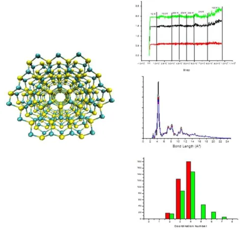
Fig 4:

Cluster di CdS has been reported together some results obtained with QDprop

In our last work, not yet published, this code has been used to analyse the trajectory from CPMD

calculations of the cluster built with 162 atoms of cadmium and 162 atoms of sulfur. Another

cluster that we would simulate is ZnS with spherical shape. The CdS cluster and some graphical

output from QDprop are reported in Figure 4.

Reference

[1] E.BURRESI, M. CELINO

“Methodological approach to study energetic and structural properties of

nanostructured cadmium sulfide by using ab-initio molecular dynamics simulations”. Solid State Science 14

(2012) pp. 567-573

[2]E. BURRESI, M. CELINO

“Surface states and electronic properties for small cadmium sulfide

nanocluste

r” (2013), Nanoscience and Nanotechnology Letters 5 pp.1182-1187

[3] E. BURRESI, M. CELINO (2014) in High Performance Computing on CRESCO infrastructure: research

activities and results 2013 ISBN: 978-88-8286-325-8

[4] E. BURRESI, M. CELINO in High Performance Computing on CRESCO infrastructure: research

activities and results 2014 (2015) ISBN: 978-88-8286-325-8

Inter-layer synchronization in multiplex

networks

I. Sendi˜

na-Nadal

_{, I. Leyva}

_{, R. Guti´}

_errez

_{, R. Sevilla-Escoboza}

_{, J.M. Buld´}

_u

_{, J.}

A. Almendral

_{and S. Boccaletti}

1

Complex Systems Group & GISC, Universidad Rey Juan Carlos, 28933 M´ostoles, Madrid, Spain

2

Center for Biomedical Technology, U. Polit´ecnica de Madrid, 28223 Pozuelo de Alarc´on, Madrid, Spain

3

Centro Universitario de los Lagos, Universidad de Guadalajara, Jalisco 47460, Mexico

4

School of Physics and Astronomy, University of Nottingham, Nottingham, NG7 2RD, UK

5

CNR- Institute of Complex Systems, Via Madonna del Piano, 10, 50019 Sesto Fiorentino, Florence, Italy

6

The Italian Embassy in Israel, 25 Hamered st., 68125 Tel Aviv, Israel

❆❜str❛❝t✳ Inter-layer synchronization is a distinctive process of multiplex networks whereby each node in a given layer evolves synchronously with all its replicas in other layers, irrespective of whether or not it is synchronized with the other units of the same layer [9]. We analytically derive the necessary conditions for the existence and stability of such a state, and verify numerically the analytical predictions in several cases where such a state emerges. We further inspect its robustness against a progressive de-multiplexing of the network.

1

Introduction

Synchronization in networked systems is one of the hottest topics of current research in nonlinear science [3, 1]. So far, most of the focus has been concentrated on systems where all the constituents are treated on an equivalent footing, while only in the last few years the interest has moved towards incorporating the multilayer character of real world networks, by representing them as graphs formed by diverse layers [5, 2], which may either coexist or alternate in time [2]. For dynamical processes, multilayer allows identifying synchronization regions that arise as a consequence of the interplay between the layers’ topologies [10], assesing the stability of a global synchronous state in a network of oscillators coupled through different variables [8], as well as defining new types of synchronization based on the coordination between layers [4]. In this work, we consider multiplex networks, i.e. the case where layers are made of a fixed set of nodes and connections exist between each node of a layer and all its replicas in the other layers, and show that a genuinely distinctive form of synchronization emerges, namely inter-layer synchronization, occurring when each unit in each layer is synchronized with all its replicas, regardless of whether or not it is synchronized with the other members of its layer.

By means of extensive calculations performed in CRESCO, in the last year we have obtained several

λ

λ

layer X

x

(t)=y

(t), x

(t)≠x

(t)

layer Y

x

(t)=y

(t), x

(t)=x

(t)

Figure 1: Schematic representation of a multiplex of two layers of identical oscillators, and of the two types of inter-layer synchronization: with (left) and without (right) intra-layer synchronization. Labels σ and λ denote the intra- and inter-layer coupling strengths, respectively. Each node i (j) in the top (bottom) layer is an m dimensional dynamical system whose state is represented by the vector xi (yj).

important results that provide new insights in the dynamics of synchronization in complex networks. The results were published in Refs. [6, 7, 9] and presented in several international conferences.

2

Model and methods

2.1

Model

We start by considering two layers of identical structure, formed by N identical m dimensional dy-namical systems whose states are represented by the vectors X = {x1, x2, . . . , xN} (top layer) and

Y = {y1, y2, . . . , yN} (bottom layer) with xi, yi, for i = 1, 2, . . . , N , as depicted in Fig. 1. As already

mentioned, the inter-layer synchronous state X ≡ Y can be realized with or without intra-layer syn-chronization. The former case (Fig. 1 left) corresponds to all nodes in both layers following the same trajectory, and it therefore reduces to the classical scenario of a globally synchronous solution whose stability can be accounted for by the Master Stability Function (MSF) [3]. The latter case (Fig. 1 right), instead, is far more general, as it only requires that every node i in each layer be synchronous to its replica in the other layer [xi(t) = yi(t), ∀i], with unconstrained intra-layer dynamics.

Let the dynamics of the multilayer system be ˙

X= f (X) − σL ⊗ h(X) + λ [H(Y) − H(X)], Y˙ = f (Y) − σL ⊗ h(Y) + λ [H(X) − H(Y)], (1) where f : Rm _{→ R}m _{and H : R}m _{→ R}m _{are respectively the intra- and interlayer coupling vectorial}

functions, σ, λ are the intra- and inte-layer coupling strengths and L is the the Laplacian matrix encoding the intra-layer topology, considered identical for both layers. In this setting, the layer’s dynamical state will be, in general, different at all times, i.e. X(t) 6= Y(t). Notice that, if the coupling between layers is diffusive, the inter-layer synchronous state always exists, and the manifold X(t) = Y(t) is an invariant set.

Let now δX(t) = Y(t) − X(t) be the vector describing the difference between the dynamics of the two layers. Considering a small δX and expanding around the inter-layer synchronous solution Y = X + δX up to first order, one obtains a set of N × m linearized equations for the perturbations δxi:

δ ˙xi= [Jf (˜xi) − 2λ JH(˜xi)] δxi− σ

X

j

0 0.05 0.1 0 100 200 300 400 500 λ Einter 0 0.05 0.1 0 500 1000 Eintra λ 0 0.05 0.1 0 100 200 300 400 500 λ Einter 0 0.05 0.1 0 500 1000 Eintra λ 0 0.05 0.1 −0.1 −0.05 0 0.05 0.1 0.15 λ MLE σ=10−4 σ=0.02 σ=0.20 σ=0.50 0.001 0.01 0.1 1 0 0.02 0.04 0.06 0.08 0.1 σ λ * ER 〈 k〉=4 ER 〈 k〉=8 ER 〈 k〉=16 SF 〈 k〉=4 SF 〈 k〉=8 SF 〈 k〉=16 d a b c

Figure 2: (a) Einter in SF layers of N = 500 R¨ossler oscillators and (c) the corresponding MLE as a

function of λ for several σ values. (b) The same as in (a) but for ER layers. Insets in (a) and (b) show Eintrain the top layer, and the vertical dashed line is the λ threshold for a pair of nodes (σ = 0) coupled

through the y variable. Each point is an average of 10 realizations, with hki = 8. (d) Dependence of the inter-layer synchronization onset, λ∗_{on σ for ER (red hollow symbols) and SF (blue solid symbols), and}

several hki. The horizontal dashed line is placed at the same value as the vertical line in panels (a)-(c).

where J denotes the Jacobian operator and ˜X= {˜xi} is the state of one isolated layer obeying ˙˜xi =

f(˜xi) − σPjLijh(˜xj). The linear equations (2), solved in parallel to the N × m nonlinear equations

for ˙˜xi, allow calculating all Lyapunov exponents transverse to the manifold X = Y. The maximum of

those exponents (MLE) as a function of the parameter pair (σ, λ) actually gives the necessary conditions for the stability of the inter-layer synchronous solution: whenever MLE< 0, perturbations transverse to the manifold die out, and the multiplex network is said to be inter-layer synchronizable.

In the following, te intra- and inter-layer synchronization errors, respectively defined as, Eintra= lim T →∞ 1 T Z T 0 X j6=1 kxj(t) − x1(t)k dt, Einter= lim T →∞ 1 T Z T 0 kδX(t)k dt (3)

and the MLE, are calculated by performing numerical simulations of Eqs. (1) and (2) respectively (kk stands for the Euclidean norm. Without lack of generality, we consider two possible kinds of topologies where both layers are either Erd¨os-Renyi (ER) or scale-free with p(k) ∝ k−3(SF), in all cases with N = 500 R¨ossler oscillators, whose autonomous evolution is given by f (x) = [−y − z, x + 0.2y, 0.2 + z(x − 9.0)].

2.2

Numerical methods and use of computational resources

For the numerical integration of the above model and the analysis of the results we use homemade C codes implementing fix-step fourth-order Runge-Kutta integration algorithms, with an optimized time step dt=0.01. The standard GCC compiler was used.

Extensive serial simulations have been performed for large parameters ranges, diverse network topologies and statistical validation of the results. The calculations were performed in Cresco 3 and Cresco 4, using the h144 queues for full multilayer simulations and h6 queues for Lyapunov exponent calculations. Homemade MatLab scripts were used for visualizing the results.

3

Numerical results

We start by setting h = (0, 0, z) so that the corresponding MSF is in class I thus preventing the occurrence of intra-layer synchronization for any possible value of σ at λ = 0. In addition, the inter-layer coupling function is taken to be H = (0, y, 0), which generates a class II MSF at σ = 0 [3]. Results are reported in Fig. 2, where Einter is plotted versus λ for several values of σ, both for SF (a)

and ER (b) topologies. In all cases, a smooth transition from an incoherent multiplex dynamics with Einter> 0 to an inter-layer synchronous evolution where Einter = 0 is observed, always in the absence of

intra-layer synchronization [insets in Fig. 2(a,b) show that Eintra remains well above zero for the whole

explored range of λ]. In Fig. 2 (c) the MLE for the SF case is plotted, showing that Einter vanishes

exactly at the same λ at which the MLE gets negative, thus confirming the validity of the analytical approach. To gather a clearer view on the impact of the network heterogeneity, Fig. 2 (d) reports the critical coupling λ∗ _{(the value of λ at the onset of inter-layer synchronization) as a function of σ,}

for both SF and ER topologies, and several average degrees. As in single layer networks, multiplexes of heterogeneous structures require smaller coupling thresholds to sustain a stable synchronous state. There is a non-monotonic relationship between the synchronization threshold and the stiffness within each layer (as measured by σ). The horizontal (vertical) dashed line in Fig. 2(d) [Fig. 2(a,b)] indicates the threshold λ∗

for the appearance of a synchronous state at σ = 0, obtained by analyzing a pair of bidirectionally coupled R¨ossler units. More rigid layers need larger inter-layer couplings to synchronize (as one would expect), but beyond a certain point in the rigidity, the trend is remarkably reversed.

5000 300 100 150 300 E inter multiplexed nodes

(a)

(b)

Figure 3: Einter vs. the number of multiplexed nodes for ER (void symbols) and SF (solid symbols)

configurations. From a full multiplex, nodes are progressively disconnected following a random (blue circles), and a decreasing (red squares) or increasing degree (teal triangles) sequence. λ = 0.1 (a) σ = 0.1, (b) σ = 1.0. Points are averages over 20 network realizations, with hki = 8.

Further insight can be gathered by exploring the robustness of the inter-layer synchronous state under a progressive de-multiplexing of the structure. Starting from the complete multiplex, we then sequentially remove the links between nodes and their replicas, until the layers become uncoupled. In Fig. 3, Einter

is reported as a function of the actual number of multiplexed nodes with a disconnecting mechanism following either a random sequence or the increasing/decreasing degree ranking. Robustness is critically dependent on the balance between the inter- and intra-layer couplings. At relatively low and balanced couplings (left panel) Einter grows as soon as the first pair of replica nodes is disconnected, regardless on

the node sequence. However, when σ considerably exceeds λ (right panel), inter-layer synchronization persists even if a large fraction of nodes are de-multiplexed. It can be seen that ER layers (void symbols) are less robust than SF layers (solid symbols), since in the last ones synchronization holds up to the point where just a fraction of the hubs are multiplexed (Fig. 3(b)).

4

Conclusion

In conclusion, we provided a full characterization of inter-layer synchronization, a novel and distinctive dynamical phenomenon occurring in multiplex networks of identical layers, in terms of its stability conditions, its relation to intra-layer synchronization and network topology, and its robustness under partial de-multiplexing of the network. Our MSF approach strictly requires that the coupled layers in the multiplex need to be identical. In the more general case of non-identical structures, a rigorous approach should be abandoned in such a case, and one should rely on some kind of (reasonable) approximations and large numerical simulations. Future work in this direction is underway in order to extend the scope of our research to more realistic scenarios.

References

[1] A. Arenas, A. D´ıaz-Guilera, J. Kurths, Y. Moreno, and C. Zhou. Synchronization in complex networks. Phys. Rep., 469:93–153, 2008.

[2] S. Boccaletti, G. Bianconi, R. Criado, C.I. del Genio, J. G´omez-Garde˜nes, M. Romance, I. Sendi˜na Nadal, Z. Wang, and M. Zanin. The structure and dynamics of multilayer networks. Phys. Rep., 544:1–122, 2014.

[3] S. Boccaletti, V. Latora, Y. Moreno, M. Chavez, and D.-U. Hwang. Complex networks: Structure and dynamics. Phys. Rep., 424:175–308, 2006.

[4] R. Guti´errez, I. Sendi˜na-Nadal, M. Zanin, D. Papo, and S. Boccaletti. Targeting the dynamics of complex networks. Sci. Rep., 2:396, 2012.

[5] M. Kivel¨a, A. Arenas, M. Barthelemy, J.P. Gleeson, Y. Moreno, and M. A. Porter. Multilayer networks. Journal of Complex Networks, 2:203–271, 2014.

[6] A. Navas, J. A. Villacorta-Atienza, I. Leyva, J. A. Almendral, I. Sendi˜na Nadal, and S. Boccaletti. Effective centrality and explosive synchronization in complex networks. Phys. Rev. E, 92:062820, 2015.

[7] I. Sendi˜na-Nadal, I. Leyva, A. Navas, J.A. Villacorta-Atienza, J.A. Almendral, Z. Wang, and S. Boccaletti. Effects of degree correlations on the explosive synchronization of scale-free networks. Phys. Rev. E, 91:032811, 2015.

[8] R. Sevilla-Escoboza, R. Guti´errez, G. Huerta-Cuellar, S. Boccaletti, J. G´omez-Garde˜nes, A. Arenas, and J M Buld´u. Enhancing the stability of the synchronization of multivariable coupled oscillators. Phys. Rev. E, 92:032804, 2015.

[9] R. Sevilla-Escoboza, I. Sendi˜na-Nadal, I. Leyva, R. Guti´errez, J.M. Buld´u, and S. Boccaletti. Inter-layer synchronization in multiplex networks of identical Inter-layers. Chaos, 26:065304, 2016.

[10] F. Sorrentino. Synchronization of hypernetworks of coupled dynamical systems. New J. Phys., 14:33035, 2012.

ATMOSPHERIC POLLUTION TRENDS SIMULATED AT

EUROPEAN SCALE IN THE FRAMEWORK OF THE

EURODELTA 3 PROJECT

Gino Briganti

, Andrea Cappelletti

, Mihaela Mircea

, Mario Adani

, Massimo D’Isidoro

1

ENEA - National Agency for New Technologies, Energy and Sustainable Economic Development, Pisa, Italy 2

ENEA - National Agency for New Technologies, Energy and Sustainable Economic Development, Bologna, Italy

ABSTRACT. The present paper shows simulations

for the years 1990, 2000 and 2010 performed with

the atmospheric modelling system (AMS) of MINNI project at European scale. The modelling system is the

reference model of Italian Ministry of Environment developed with the aim to support air quality policy

at national and regional level.

The work has been carried out in the framework of EURODELTA 3

project, phase 2, designed to investigate the evolution of air pollution since the early 1990s.

1 Introduction

The EU directive 2008/50/EC promotes modelling techniques in order to assess spatial distribution

of the ambient air quality, even in place of measurements where lower pollution levels are expected.

Air quality models are considered as essential tools, helping to develop emissions control plans, in

order to guarantee better air quality levels and to preserve both human health and ecosystems. Since

such models incorporate advection/dispersion drivers, coupled with complex chemistry solvers,

they require a lot of computation resources; supercomputing architectures, like CRESCO, are then

the ideal infrastructure to run them.

The present paper presents the preliminary results achieved by the ENEA’s MINNI [1] team in

simulating trends on atmospheric pollution at European scale. MINNI is the Italian Integrated

Assessment Modelling System for supporting the International Negotiation Process on Air Pollution

and assessing Air Quality Policies at national/local level, sponsored by the Italian Ministry of the

Environment.

The work has been carried out under the “Trends” phase of the EURODELTA project [2]. Such

project is a forum in which European modelling groups share experiences in simulating technically

interesting and policy relevant problems, in order to get further understanding in modeling air

quality in Europe. EURODELTA is a scientific activity in the framework of EMEP Task Force on

Measurement and Modelling [3], under the Convention on Long-range Transboundary Air

Pollution.

The focus of EURODELTA-Trends is to assess the efficiency of the Gothenburg protocol in

reducing exposure to air pollution in Europe. The exercise also aim to disentangle the role of

meteorological variability, long range transport (boundary conditions) and emissions by performing

simulations as follows: i) varying emissions (years 1990, 2000, 2010) bringing both meteorology

and boundary conditions fixed (year 2010); ii) varying emissions and boundary conditions (years

1990, 2000, 2010), bringing meteorology fixed (year 2010); iii) varying boundary conditions (years

1990, 2000, 2010) with both meteorology and emissions fixed (2010); iv) other additional

simulations for completing the decomposition of factors.

2 Modeling set-up

Air quality simulations have been conducted with FARM (Flexible Regional Atmospheric Model)

[5] [6], developed by ARIANET s.r.l. (

http://www.aria-net.it/

) in Fortran 77/90 language. FARM is

a three-dimensional Eulerian grid model with K-type turbulence closure that accounts for the

transport, chemical reactions and ground deposition of atmospheric pollutants. The version used is

4.7, with SAPRC99 [7] gas phase chemical mechanism and AERO3 [8] aerosol model; this version

have been recently rewritten in order to support hybrid MPI-OpenMP parallelization [9].

Grids specifications for FARM simulations are shown in Table 1. Horizontal coordinates are in

latitude/longitude, whereas vertical levels are in meters above the ground.

SW corner

(-17°E,32°N)

(NX, NY, NZ)

(143,153,16)

Vertical Z levels [m]

Quasi-logarithmic: 20, 75, 150, 250, 380, 560,

800, 1130, 1570, 2160, 2970, 4050, 5500, 7000,

8500, 10000

(∆X, ∆Y)

(0.4°,0.25°)

Table 1: Characteristics of the computational domain.

Meteorological, boundary conditions and emissions data were supplied to all participants at the

EURODELTA exercise and they have been processed to be used as input in FARM.

All the input/output data have been stored in the gporq1_minni file system. Table 2 summarizes the

settings and the resources employed on the Cresco grid adopted in each step described below.

Process

Cores Queues

Elapsed time

Disk space

Boundary

conditions

1

cresco4_h6

~ 20’/year

1.6 GB/year

Meteorology

-

local

-

200 GB/year

SURFPRO

1

cresco4_h144

~ 45’/year

115 GB/year

cresco3_h144

~ 1h20’/year

Emission Manager

12

cresco4_h6

~ 2h/year

400 GB/year

cresco3_h144

~ 4h/year

FARM

16

cresco4minni_h24

~ 1÷1.5 day/year

depending

on

Grid

crowding and other I/O

simultaneous processes.

220 GB/year

Post-processing

1

cresco4_h144

cresco3_h144

cresco4_h6

~ 2÷3 day/year

38 GB/y