Article
A Spatial-Filtering Zero-Inflated Approach to the
Estimation of the Gravity Model of Trade
Rodolfo Metulini1 ID, Roberto Patuelli2,3,*ID and Daniel A. Griffith4 ID
1 Department of Economics and Management, University of Brescia, 25122 Brescia, Italy; [email protected]
2 Department of Economics, University of Bologna, 40126 Bologna, Italy
3 The Rimini Centre for Economic Analysis (RCEA), Waterloo, ON N2L3C5, Canada
4 School of Economic, Political & Policy Sciences, The University of Texas at Dallas, Richardson, TX 75080, USA; [email protected]
* Correspondence: [email protected]; Tel.: +39-0541-434276
Received: 23 September 2016; Accepted: 12 February 2018; Published: 22 February 2018
Abstract: Nonlinear estimation of the gravity model with Poisson-type regression methods has become popular for modelling international trade flows, because it permits a better accounting for zero flows and extreme values in the distribution tail. Nevertheless, as trade flows are not independent from each other due to spatial and network autocorrelation, these methods may lead to biased parameter estimates. To overcome this problem, eigenvector spatial filtering (ESF) variants of the Poisson/negative binomial specifications have been proposed in the literature on gravity modelling of trade. However, no specific treatment has been developed for cases in which many zero flows are present. This paper contributes to the literature in two ways. First, by employing a stepwise selection criterion for spatial filters that is based on robust (sandwich) p-values and does not require likelihood-based indicators. In this respect, we develop an ad hoc backward stepwise function in R. Second, using this function, we select a reduced set of spatial filters that properly accounts for importer-side and exporter-side specific spatial effects, as well as network effects, both at the count and the logit processes of zero-inflated methods. Applying this estimation strategy to a cross-section of bilateral trade flows between a set of 64 countries for the year 2000, we find that our specification outperforms the benchmark models in terms of model fitting, both considering the AIC and in predicting zero (and small) flows.
Keywords: bilateral trade; unconstrained gravity model; eigenvector spatial filtering; zero flows; backward stepwise; zero-inflation
JEL Classification:C14; C21; F10
1. Introduction
A traditional gravity model describing trade in its simple form asserts that the volume of trade between a country pair is proportional to the product of their gross domestic products and inversely related to a measure of distance separating them, where distance is broadly defined as a function of several variables that can be viewed as trade resistance factors. The log-linear specification of the gravity model along with ordinary least squares (OLS) estimation has been widely used in the empirical literature (for a wide review, seeHead and Mayer 2014), mostly because of its good empirical performance and, in later years, for the strong theoretical foundations provided in papers such as Anderson(1979) andAnderson and Wincoop(2003). A “structural break” in applied trade modelling is represented by the work ofSantos Silva and Tenreyro(2006), who show that log-linearization of the gravity model leads to inconsistent estimates in the presence of heteroscedasticity in trade
levels (and because of Jensen’s inequality). They propose a Poisson-type specification of the gravity model along with a Poisson pseudo-maximum likelihood (PPML) estimator, somehow similarly to the Poisson approach proposed much earlier byFlowerdew and Aitkin(1982).Santos Silva and Tenreyro (2006,2011) also provide simulation evidence that the PPML estimator is well-behaved even when the conditional variance is far from being proportional to the conditional mean. Several studies in trade have since then applied the PPML estimator (seeLinders et al. 2008;Martin and Pham 2015; Burger et al. 2009;Martínez-Zarzoso 2013).
A further aspect stressed in recent contributions is the one of null trade flows and the necessity to specifically take them into account in regression modelling. Helpman et al. (2008) prove that disregarding countries that do not trade with each other generates biased estimates. Zero-inflated specifications of Poisson models (ZIP) (Lambert 1992;Greene 1994;Long 1997) permit to explicitly model the presence of a large number of zero flows, because it considers the existence of two groups within the population: one having strictly zero counts, and another having a non-zero probability of having a trade flow greater than zero. In this framework, a relevant question is whether the determinants of zero flows are the same as the ones of trade counts. Indeed,Burger et al.(2009) stress that some variables (such as common language, institutional and geographical distance) may be more important in determining the profitability of bilateral trade (decision to trade) rather than the potential volume of bilateral trade. Nordås(2008), on the other hand, employed the same variables in both model parts, in an empirical application focusing on trade liberalization. However, so far, which variables determine the decision to trade is not so clear, and models may suffer from omitted variables bias in either one of model parts, or both.
A second issue taken up in this paper is trade flows interdependence (Griffith 2007;LeSage and Pace 2008), which is reflected in network autocorrelation among flows or, looking at the marginal sums of trade matrices, spatial autocorrelation (SAC) among countries (Behrens et al. 2012;Sellner et al. 2013). Behrens et al.(2012), in particular, provide a theoretical discussion and empirical testing showing that multilateral trade resistance (MTR) terms can be accounted for as SAC in spatial model specifications. In this paper, we aim to analyze the dynamics of the decision to trade (extensive margin) and the volume of trade (intensive margin), and, in particular, what the contribution of SAC is in both of these processes. We focus on an eigenvector spatial filtering (ESF) approach (Griffith 2003), within a ZIP framework, using two sets of origin, destination and network spatial filters (Griffith 2007;Fischer and Griffith 2008), one accounting for SAC in the logit part, and the other accounting for SAC in the count part. In this regard, we devise an ad hoc function that applies a backward stepwise algorithm aiming to properly identify the significant spatial filters. Our proposed algorithm has the advantage that, at each step, it drops the eigenvector with the largest p-value, regardless of whether it is in the count or in the logit part. We compare the results of this estimation with two methodologically nested benchmarks, namely a ZIP without ESF in the logit part (ZIP ESFc) and a Poisson with ESF (Poisson ESF). We conduct a comparison in terms of both estimated coefficients and goodness of fit (Akaike information Criteria, AIC and prediction of zero and small flows). We find that our specification outperforms the comparison models, in terms of both AIC and prediction of small trade flows. We stress that our proposed method can be of practical help in applied trade modelling, in particular when trade flows with a high share of zeros are to be used.
This paper is structured as follows. Section2presents a review of the gravity of trade, from the traditional models to recent developments. In Section3, we define our proposed model and the stepwise algorithm we adopted. Section4presents the empirical application, together with results. Section5concludes the paper.
2. The Gravity Model of Trade: Recent Developments
The scientific community recently experienced a renewed interest in both the theoretical and empirical aspects of the gravity model of trade. In particular, the aforementioned theoretical developments on multilateral resistance terms generated the need for consistent estimation approaches
that would fit such advancements. The vastly increased computational power available for econometric analysis played an additional role, allowing more complex and data-intensive (i.e., nonlinear and panel) estimation efforts.
Several studies, starting with, for example, the popular paper bySantos Silva and Tenreyro (2006), have pushed the envelope in the field, and a number of researchers are actively pursuing further methodological advances pertaining to, in particular, the estimation of the gravity model of trade.Egger and Tarlea(2015) propose a multi-way clustering approach to consistently estimate the regression coefficients’ standard errors pertaining to preferential trade agreements.Egger and Staub (2016) compare the suitability of various estimation approaches under an international economics general equilibrium perspective. Baltagi and Egger(2016) develop a quantile regression structural estimation solution for the gravity model.
Within the aforementioned econometric developments, a niche of its own is emerging pertaining to the incorporation of spatial dependence and heterogeneity or network autocorrelation (i.e., the correlation of flow data based on their network’s topological characteristics) in gravity models (Patuelli and Arbia 2016), trade being a frequent application. While the relevance of spatial autocorrelation originally was suggested for trade models inAnderson and Wincoop(2004), and much earlier within spatial interaction modelling (Curry 1972;Curry et al. 1975;Sheppard et al. 1976), this issue attracted significant attention only in recent years. Studies byBehrens et al.(2012),Fischer and Griffith(2008), andLeSage and Pace(2008) provide, from different perspectives (economic theory, spatial econometrics, spatial statistics), the necessary stepping stones for analyzing SAC aspects in flow data. We can roughly divide the available literature into three main streams:
• Linear spatial econometric models (LeSage and Pace 2008;Behrens et al. 2012;Fischer and Griffith 2008;Baltagi et al. 2007;Koch and LeSage 2015): these models apply and adapt traditional (linear) spatial econometric techniques to the count data case.
• Spatial generalized linear models (GLMs) (Sellner et al. 2013;Lambert et al. 2010): these models extend the previous approaches by allowing for estimation based on Poisson-type models, therefore accommodating the concerns expressed inSantos Silva and Tenreyro(2006).
• Semi-parametric (ESF) models (Fischer and Griffith 2008;Scherngell and Lata 2013;Krisztin and Fischer 2015;Chun 2008;Patuelli et al. 2016): these models mix a parametric and a non-parametric approach, by employing ESF within Poisson-type models.
This paper is concerned with this latest class of models. ESF (Griffith 2003) (described in more detail in Section3.2) is a spatial statistics technique based on the decomposition of spatial weights matrices. The available studies employing this technique demonstrate how spatial filters can be used successfully at the intercept level as “interceptors” of (i.e., proxies for) unobserved spatial heterogeneity (Patuelli et al. 2012). With particular regard to our modelling exercise, ESF can be used to approximate the fixed effects that, in a cross-sectional model of bilateral trade, would be estimated by sets of country dummies. This paper aims to further investigate the use of ESF, by allowing for separate spatial filter sets in zero-inflated models.
3. A Methodological Approach 3.1. Zero-Inflated Gravity Models of Trade
In recent years, there is an increasing recognition that the level of trade between countries frequently is zero. Small countries may not have trade relations with all possible trading partners, or statistical offices may not report trade flows below a certain threshold. Moreover, the issue of zero flows is more pronounced when analyzing sector-disaggregated trade flows. Zero-inflated gravity models provide one way to model an excess of zero flows. Martin and Pham (2015) and Burger et al.(2009) propose the zero-inflated extension of the Poisson gravity model for situations where the data-generating process (DGP) results in too many zeros. The model may be viewed as a
“two-part” extension, in which the distribution of the outcome variable is approximated by mixing two component distributions. The zero-inflation part of the model consists of a qualitative-dependent model to determine the probability of whether a particular origin-destination trade flow is zero or positive. The second part contains the standard Poisson (or negative binomial) gravity model to estimate the relationship between trade flows and explanatory variables for each trade flow that has a non-zero probability (Leung and Yu 1996). Among others, Xiong and Beghin (2012) and Philippidis et al.(2013) apply zero-inflated count models for the analysis of international trade.
Estimating the parameters of Poisson-type gravity models (with or without zero-inflation) by standard non-spatial methods only is justified statistically if we believed that trade flows are independent observations. However, such an assumption generally is not valid because flows fundamentally are spatial in nature. Several recent papers propose modelling the spatial heterogeneity in the residuals by means of different econometric techniques. Among those works, many focus on the issue of MTR, which can be considered as a main source of spatial heterogeneity (Behrens et al. 2012; Baier and Bergstrand 2009). One way to relax this independence assumption is by incorporating spatial dependence in the Poisson gravity model by means of spatial autoregressive techniques (Sellner et al. 2013;Lambert et al. 2010). Another is ESF (Griffith 2003). It is considered here because it allows for greater flexibility in modelling, and can be applied seamlessly to any estimation framework. In their recent work, Patuelli et al. (2016) apply spatial filters within a negative binomial (NB) specification as a way to filter out spatial heterogeneity due to MTRs. However, residual heterogeneity could be present both for the logit and the count process, whereas the previously mentioned works only account for SAC in the count process. Krisztin and Fischer(2015) have very recently applied network-autocorrelation SFs to a trade model, by including, among others, zero-inflated specifications. In particular, their approach implies using a network autocorrelation spatial filter in the count part of the model. This work follows a similar approach used byKrisztin and Fischer (2015), but we introduce an ad hoc backward stepwise procedure to properly select the filters. Moreover, we perform diagnostics in order to: (i) compare our model with other benchmarks; and (ii) evaluate the fitting of our specification in predicting zero (and small) trade flows.
3.2. Spatial Filters
ESF originally was developed for area-based data byGriffith(2003), and later extended to flow data (Fischer and Griffith 2008;Chun 2008;Chun and Griffith 2011;Griffith 2009). One traditional advantage, when including eigenvectors as additional origin- and destination-specific regressors, is that the model can be estimated within standard regression frameworks, such as OLS or Poisson regression, which are common in the literature about spatial interaction. The parameters of the standard regressor variables are unrelated to the remaining residual term, and standard estimation yields consistent parameter estimates as a result. We refer to this estimation method as SF estimation of origin-destination models.
The workhorse for the SF decomposition is a transformation procedure-based upon eigenvector extraction from the matrix
(I−11T/n) W (I−11T/n) (1)
where W is a generic n×n spatial weights matrix with zeros on the main diagonal. I is an n×n identity matrix, and 1 is an n×1 vector containing 1s. The spatial weights matrix W defines the relationships of proximity between the n georeferenced units (e.g., points, regions, and countries). The transformed matrix appears in the numerator of the Moran I coefficient (MC).
The eigenvectors of Equation (1) represent distinct map pattern descriptions of SAC underlying georeferenced variables (Griffith 2003). Moreover, the first extracted eigenvector, say e1, is the one showing the highest positive MC (Cliff and Ord(1972,1981)) that can be achieved by any spatial recombination induced by W. The subsequently extracted eigenvectors maximize MC while being orthogonal to and uncorrelated with the previously extracted eigenvectors. Finally, the last extracted eigenvector maximizes negative MC.
Having extracted the eigenvectors of Equation (1), a spatial filter is constructed as a linear combination of a judiciously selected subset of these n eigenvectors. In detail, for our empirical application, when it comes to origin/destination ESF, we select a first subset of eigenvectors (which we call the “candidate eigenvectors”) by means of the following threshold: MC(ei)/MC(e1) > 0.25. This threshold corresponds to a percentage of variance of at least 5 per cent being explained by the dependent variable’s spatial lag (WY on Y), according to (Griffith 2003). With regard to network ESF, the algorithm proposed byChun et al.(2016) has been employed.1Subsequently, a stepwise regression model may be employed to further reduce the first subset (whose eigenvectors have not yet been related to given data) to just the subset of eigenvectors that are statistically significant as regressors in the model to be evaluated. The linear combination of the resulting group of eigenvectors is what we call our “spatial filter”.
Because trade data do not represent points in space, but flows between points, the eigenvectors are linked to the flow data by means of Kronecker products: the product EK⊗1, where EKis the n×k matrix of candidate eigenvectors, may be linked to the origin-specific information (for example, GDP per exporting countries), while the product 1⊗EKmay be linked to destination-specific information (again, for example, the gross domestic product of importing countries) (Fischer and Griffith 2008). As a result, two sets of origin- and destination-specific variables are used (Patuelli et al. 2016), which aim to capture the SAC patterns commonly accounted for by the indicator variables of a doubly-constrained gravity model (Griffith 2009), therefore avoiding omitted variable bias see also Griffith and Chun(2016).
The new challenge here is that we want to account for SAC in both the logit and in the count parts of zero-inflated models, so we use two sets of filters at the logit level, and two sets of filters at the count level. This choice allows us to account for potentially different omitted variables related to the intensive and extensive margins of trade. Moreover, the selection of different eigenvectors in the two parts (i.e., exclusion restrictions) may help obtain identification as well, consistently with Papadopoulos and Silva(2012).
3.3. A Backward Stepwise Algorithm
A stepwise procedure is an algorithm used to choose variables in a regression model, first proposed byEfroymson(1960). It usually takes the form of a sequence of F- or t-tests, but other criteria are possible, such as (adjusted) R-squared, AIC, Bayesian information criterion (BIC), or simply based on p-values.
Forward selection involves starting with no variables in a model, testing the addition of each variable, adding the variable (if any) that improves the model the most, and repeating this process until no more (significant) improvement is possible. Backward elimination involves starting with all candidate variables, sequentially testing the deletion of each of them, deleting the variable (if any) whose deletion improves the model fit the most, and repeating this process until no further improvements are possible. Backward elimination procedures are implemented in many routines. Chun and Griffith(2013) listRcode for stepwise selection in GLMs based on SAC minimization. In thempathpackage (Wang et al. 2015), thebe.zeroinflfunction performs a backward elimination (and forward selection) based on maximum likelihood criteria, and can be applied to zero-inflated models. Further variable selection algorithms for zero-inflated count data are presented in the medical literature, all proposing LASSO-based approaches (Chen et al. 2016;Zeng et al. 2014;Buu et al. 2011) with different types of penalizations. None has been proposed in economics or other fields of research, to the authors’ best knowledge.
1 The equation formulated byChun et al. (2016), based on residual SAC, predicts the ideal size of the set of candidate
Here, we are interested in using a stepwise algorithm to define the proper set of eigenvectors to include in a regression model in order to account for SAC. Our algorithm is based on thebe.zeroinfl
function, but has at least two advantages vis-à-vis it. First, at each step of our algorithm, we compute robust standard errors as in PPML models, and we select the variable to be removed based on the related p-values. Second, our algorithm is constructed in order to be able to drop the variables with the largest p-values, regardless of whether they belong to the count or the logit part. We also structured the function so that a minimum model (minmodel) can be defined. In other words, we let the algorithm drop only the eigenvectors, because we consider included standard explanatory variables to have substantive meaning.
In particular, our algorithm can be depicted by the following description and pseudo-code reported in Box1.
Box 1.Description of the algorithm.
Usage
Backward.Stepwise.Zeroinfl(object, data, dist = ("poisson", "negbin", "geometric"), alpha = 0.05, trace = TRUE, subset.zero, subset.count, minmod.zero, minmod.count)
Arguments
object: an object from functionzeroinfl
data: adata.frameobject containing the variables to be used in the regression model
dist: one of the distributions used in thezeroinfl function. This could be “poisson”, “negbin” or “geometric”
alpha: the significance level for variable elimination trace: if true, it generates printed detailed calculation results
subset.zero: a list of the variable names to be subset in the logit part of the model subset.count: a list of the variable names to be subset in the count part of the model minmod.zero: a list of the variable names not to be subset in the logit part of the model minmod.count: a list of the variable names not to be subset in the count part of the model Pseudo code
Ifobjectis not ofzeroinflclass
Stop. Message: “Object must bezeroinfl”;
If the listc(subset.count, minmod.count)is not identical to the list of variables in the count part of the zeroinflobject
Stop. Message: “The count part variables inobjectmust be equal to the variables inminmod.countplus the variables insubset.count”;
If the listc(subset.zero,minmod.zero) is not identical to the list of variables in the logit part of the zeroinflobject
Stop. Message: “The logit part variables in object must be equal to the variables inminmod.zeroplus the variables insubset.zero”.
Fit thezeroinflmodel defined inobject(the “initial” model) using the distribution defined indist; Generate robust “sandwich” standard errors of the initial model, with PPML adjustment;
Print the initial model results with BIC, AIC and log-likelihood; Cycle
Print the number of the step (the initial model corresponds to step 1);
Choose the smallest p-value for the variables insubset.count(count.max) and the smallest p-value for the variables insubset.zero(zero.max);
Ifcount.maxis larger thanzero.maxand larger thanalpha The variable related tocount.maxis dropped from the model; The dropped variable’s name is removed fromsubset.count; A newobjectvalue is generated by replacing the newsubset.count; “Drop variable in count component: variable name” is printed; Else, ifzero.maxis larger thanalpha
The variable related tozero.maxis dropped from the model; The dropped variable’s name is removed fromsubset.zero; A newobjectvalue is generated by replacing the newsubset.zero; “Drop variable in zero component: variable name” is printed; Refit thezeroinflmodel using the updatedobjectvalue;
Generate robust “sandwich” standard errors of the updatedzeroinflmodel, with PPML adjustment; Print the updatedzeroinflmodel results with BIC, AIC and log-likelihood;
Restart the cycle, until bothcount.maxandcount.maxare equal or smaller thanalpha; End cycle
4. An Empirical Application
The data for trade analyzed in this paper are from the World Trade Database, compiled on the basis of COMTRADE data byFeenstra et al.(2005). GDP and per capita GDP data are from the World Bank’s WDI database. Distance, language, colonial history, landlocked countries, and land area data are from the CEPII institute. Whether pairs of countries take part in a common regional integration agreement (FTA) was determined on the basis of OECD data about major regional integration agreements.2 An indicator variable measures whether a pair of countries has (membership in) at least one common FTA. Data about island status have been kindly provided by Hildegunn Kyvik-Nordas (fromJansen and Nordås 2004). Internal flows are excluded from our analyses because they typically deserve special treatment in trade models (see, e.g.,LeSage and Fischer 2016). Their treatment within our modelling framework is left for future research.
4.1. The Model Specification
For estimation, we follow a standard specification of the gravity equation of bilateral trade, and we employ some variables commonly used in the literature. We use the following standard specification of the gravity equation, which we estimated by means of a ZIP of the form:
Pr[γk|zk, xk] = ( θk(xk) + [1−θk(xk)]exp(−µk)i f γk=0 [1−θk(xk)]exp(−µγk!k)µki f γk >0 (2a) θk(xk) = exp(xkγ) 1+exp(xkγ) (2b)
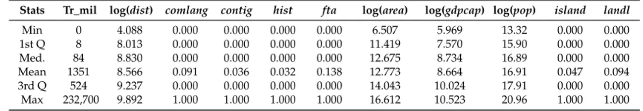
where xkis a vector of covariates defining the probabilities γkand θkof trade flows (in thousands of dollars), where γkand θkare included in [0, 1]. The vector of covariates consists of pop, that represents each country’s population (in logs), gdpcap, that represents per capita GDP (in logs), island, an indicator variable that equals 1 if a country is an island, area, that is the land area of a country (in logs), and landl, that equals 1 for landlocked countries. The other variables are country-pair indicators, identifying whether a pair of countries share a currency (comcur), the same language (comlang), a common border (contig), a common colonial history (hist), that represents if the country pair shares any history of colonization (including one colonizing the other), or engage in free trade agreements (fta), and dist is a measure of the geographical distance between them (in logs). Summary statistics are provided in Table1.
Table 1.Summary statistics for the variables used in the analysis.
Stats Tr_mil log(dist) comlang contig hist fta log(area) log(gdpcap) log(pop) island landl
Min 0 4.088 0.000 0.000 0.000 0.000 6.507 5.969 13.32 0.000 0.000 1st Q 8 8.013 0.000 0.000 0.000 0.000 11.419 7.570 15.90 0.000 0.000 Med. 84 8.830 0.000 0.000 0.000 0.000 12.675 8.734 16.89 0.000 0.000 Mean 1351 8.566 0.091 0.036 0.032 0.138 12.773 8.664 16.91 0.047 0.094 3rd Q 524 9.237 0.000 0.000 0.000 0.000 14.043 10.024 17.91 0.000 0.000 Max 232,700 9.892 1.000 1.000 1.000 1.000 16.612 10.523 20.96 1.000 1.000 4.2. Estimation Results
We estimate Equation (2) and select spatial filters as a ZIP, using a cross-section of 64 countries (4032 country pairs) for the year 2000 (ZIP ESF, 2). We estimate the same model using two benchmarks that methodologically can be considered as special cases of our proposed model: a ZIP using spatial
2 An ever-updated list of trade agreements can be accessed from the World Bank website athttps://wits.worldbank.org/
filters only in the count part (ZIP ESFc), and a Poisson with spatial filters (Poison ESF).3Two additional (simpler) benchmark models are proposed in AppendixB, that is, a standard ZIP and a Poisson with origin and destination fixed effects. Our code and the proposed algorithm are available on the first author’s personal website.
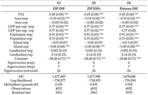
Looking at the Poisson part (second step) of the ZIP ESF in Table2, distance has a negative significant effect, the country-pair indicator variables present positive and significant coefficients, as expected: GDP positively affects trade flows, at both the exporter and importer country side. Geographical size of the importer also has a positive effect, though much smaller than for GDP. Bilateral proximity indicators, such as contiguity, common history and FTAs, all influence positively the amount of trade. Island status has a negative effect at the exporter side, but no significant effect is found for importers. Distance has the expected negative sign. The negative sign on per capita GDP is of more difficult interpretation, but constant over the benchmark models. It could imply a tendency of richer countries to produce internally most goods because of differentiation. When comparing the findings of Model (1) with the ones of the benchmarks, coefficients are very stable.
Table 2.Estimated coefficients for: (1) ZIP ESF; (2) ZIP ESFc; (3) Poisson ESF.
(1) (2) (3)
ZIP ESF ZIP ESFc Poisson ESF
First Step (logit)
Distance 0.57 (0.16) *** 0.34 (0.08) *** – Common language −0.73 (0.30) ** 0.29 (0.22) – Contiguity 0.54 (0.52) 0.13 (0.53) – Common history −0.09 (0.76) −1.43 (0.80) * – FTA −2.51 (0.50) *** −1.44 (0.35) *** – Area imp 0.32 (0.08) *** 0.05 (0.05) – Area exp 0.09 (0.06) 0.29 (0.05) *** –
GDP per cap. imp −1.35 (0.11) *** −0.73 (0.05) *** – GDP per cap. exp −0.89 (0.09) *** −0.83 (0.07) *** – Population imp −1.02 (0.12) *** −0.43 (0.08) *** – Population exp −1.01 (0.10) *** −1.15 (0.08) *** – Island imp −0.48 (0.64) −1.12 (0.41) *** – Island exp 0.44 (0.54) −1.71 (0.47) *** – Landlocked imp 3.74 (0.48) *** −0.12 (0.18) – Landlocked exp −0.15 (0.31) −1.08 (0.23) *** – Constant 38.69 (3.27) *** 30.48 (2.32) *** – Eigenvectors (exp) 10 – – Eigenvectors (imp) 16 – – Eigenvectors (network) 28 – –
Second Step (Poisson)
Distance −0.58 (0.04) *** −0.58 (0.04) *** −0.58 (0.04) *** Common language 0.09 (0.08) 0.09 (0.08) 0.09 (0.08)
Contiguity 0.56 (0.10) *** 0.56 (0.10) *** 0.56 (0.10) *** Common history 0.19 (0.09) ** 0.19 (0.09) ** 0.19 (0.09) **
3 Additional benchmark models based on simple origin and destination fixed effects (as inPatuelli et al. 2016) were tested,
but in a zero-inflated setting appear to cause multicollinearity issues. Indeed, the current econometric literature is very sparse with regard to the use of fixed effects in ZIP models, with onlyGilles and Kim(2017) and still-unpublished work (Kitazawa 2014;Majo and van Soest 2011) providing first-ever solutions. Additionally, the bilateral nature of trade data and its consequent fixed effects configuration makes such an endeavour further complicated. Consequently, the fixed effects were dropped and we chose to focus, in our comparison, on the role of spatial filters in the zero-inflation part of the models.
Table 2. Cont.
(1) (2) (3)
ZIP ESF ZIP ESFc Poisson ESF
FTA 0.45 (0.08) *** 0.45 (0.08) *** 0.45 (0.08) *** Area imp −0.19 (0.02) *** −0.19 (0.02) *** −0.19 (0.02) *** Area exp −0.003 (0.02) −0.003 (0.02) −0.003 (0.02) GDP per cap. imp 0.77 (0.03) *** 0.77 (0.03) *** 0.77 (0.03) *** GDP per cap. exp 0.77 (0.02) *** 0.77 (0.02) *** 0.77 (0.02)
Population imp 0.91 (0.03) *** 0.91 (0.03) *** 0.91 (0.03) *** Population exp 0.73 (0.03) *** 0.73 (0.03) *** 0.73 (0.03) *** Island imp −0.03 (0.07) −0.03 (0.07) −0.0 3 (0.07) Island exp −0.49 (0.08) *** −0.49 (0.08) *** −0.49 (0.08) *** Landlocked imp 0.002 (0.10) 0.002 (0.10) 0.002 (0.10) Landlocked exp 0.14 (0.10) 0.14 (0.10) 0.14 (0.10) Constant −28.48 (0.71) *** −28.48 (0.71) *** −28.48 (0.71) *** Eigenvectors (exp) 6 6 6 Eigenvectors (imp) 7 7 7 Eigenvectors (network) 24 24 24 AIC 1,477,400 1,477,988 1,478,688 Log-likelihood −738,577 −738,925 −739,290 McFadden’s pseudo-R2 0.935 0.935 0.935 Observations 4032 4032 4032 Residual dof 3910 3963 3978
***, **, * denote statistical significance at the 1, 5, 10 per cent level. Standard errors in parenthesis.
When considering the Logit part (first step) it should be remembered that it is the probability of excess zeros being modelled, so the estimated coefficients, in order to be concordant with the ones in the count model part, should have opposite signs (Lambert 1992;Preisser et al. 2012). Therefore, the probability of a country pair to be involved in trade negatively depends on distance and on the importer being landlocked, while it depends positively on FTAs and common language, as well as on the importer country’s areas, wealth (per capita GDP) and economic size (GDP). The latter favor trade also on the exporter’s side. Moreover, the coefficients resulting from the alternative zero-inflated specification [Model (2), which does not include spatial filters in the logit part] often differ from the ones for Model (1), suggesting that the inclusion of the spatial filters has a relevant role. These results highlight the need to better analyze the determinants of trade decisions.
Based on the AIC and the log-likelihood values, our model specification outperforms the benchmarks. In terms of AIC, the ZIP ESF has the lowest value (1,477,400), meaning it performs better than the benchmarks (1,477,988 for the ZIP ESFc, and 1,478,688 for the Poisson ESF). The same holds for the log-likelihood−738,577 compared to−738,925 and−739,290, respectively. Only the Poisson model with fixed effects, in TableA1, slightly surpasses the ZIP ESF in likelihood, because of the obvious mechanics of the fixed effects.
We can now analyze the robustness of our model in terms of fitting small trade flows. We compare the observed frequencies of small flows with their estimated counterparts (fitted values rounded to integers) obtained for all the models. Because one advantage of our model specification is that it should better predict small flows, we expect it to outperform the two benchmark models in this regard, especially if small flows are spatially autocorrelated. Results reported in Table3confirm this expectation. The ZIP ESF predicts 485 out of 484 zero flows, whereas the Poisson ESF predicts only 470 zero flows. The ZIP ESFc, using only count-level spatial filters, predicts 483 zero flows, despite it is more efficient in predicting other small flows, compared to the ZIP ESF. The comparison becomes more evident in TableA2, where the limits of the standard ZIP and fixed-effects Poisson models are shown in terms of predicting small and zero flows, respectively.
Table 3.Counts of observed versus predicted values.
Trade Flow
(in US$ Millions, Rounded) 0 1 2 3 4 5 6 7 8 9
Observed 484 136 112 76 64 39 42 49 35 29 ZIP ESF 485 8 12 15 18 19 20 20 20 20 ZIP ESFc 483 10 15 18 20 21 21 21 21 21 Poisson ESF 470 17 24 27 29 29 29 29 28 27
The spatial part of the model, with the ZIP ESF we select in the logit part, comprises 10 exporter-side, 16 importer-side and 28 network eigenvectors. In the count part, the number of significant eigenvectors is 6 for the exporter countries, 7 for the importer countries and 24 for country pairs.
A Moran test can be conducted on each of the four country-specific spatial filters, which are obtained as the linear combinations of the selected eigenvectors multiplied by their respective estimated coefficients. The one including the largest number of significant eigenvectors (16) appears to be the one with the lowest MC (0.050). The sets of eigenvectors with the highest MC values are the count part ones (MC = 0.205, with 7 eigenvectors, and MC = 0.261, with 6 eigenvectors, for importer- and exporter-side, respectively). The relationship between the number of eigenvectors selected and the strength of the proxied SAC appears to require further investigation, in order to better interpret the modelled patterns and educate expectations about the number of degrees of freedom to be used for the computation of spatial filters.
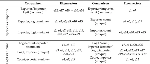
A further dimension to be investigated is the differentiated use of the eigenvectors in the construction of the spatial filters, at the importer/exporter and logit/count levels, which can provide hints regarding the extent of omitted explanatory variables and their overlap across contexts. A comparison of importer and exporter spatial filters (Table4) implies that more common eigenvectors are present in the logit part of the model. This finding suggests that (omitted) trade determinants are more differentiated, in terms of emissiveness and attractiveness, on the intensive margin. When looking at differences between the logit and count parts of the model, almost the same number of common eigenvectors can be found for the exporter and importer sides, showing that a moderate amount of omitted information is relevant for both extensive and intensive margins. More generally, no eigenvectors are in common to all four spatial filters, while out of the top three eigenvectors (e1–e3), only e1 (the one implying the spatial pattern with the highest level of SAC) appears in more than one spatial filter. These final findings lead us to believe that unexplained trade patterns are mostly idiosyncratic or tied to specific areas, rather than linked to larger geographical agglomerations (which would favor the selection of the aforementioned top eigenvectors).
Table 4.Common and unique country-specific eigenvectors.
Comparison Eigenvectors Comparison Eigenvectors
Exporter
vs.
Importer
Exporter/importer,
logit (common) e12, e17, e20, −e10, e24
Exporter/importer,
count (common) e1, e7
Exporter, logit (unique) e1, e3, e5, e9, e10, e15 Exporter, count
(unique) e4, e5, e10, e19
Importer, logit (unique) e2, e4, e7, e13, e14, e19, e20, e22, e25–e29
Importer, count
(unique) e8, e14, e20, e23, e25
Logit
vs.
Count
Logit/count, exporter
(common) e1, e5, e10
Logit/count,
importer (common) e7, e14, e20, e25 Logit, exporter (unique) e3, e9, e12, e15, e17,
e20, e24
Logit, importer (unique)
e2, e4, e12, e13, e17, e19, e22, e24, e27–e29 Count, exporter (unique) e4, e7, e19 Count, importer
5. Conclusions
Eigenvector spatial filtering (ESF) variants of nonlinear gravity models of trade (such as Poisson or NB specifications) have been proposed in the literature, because trade flows are not independent and contain spatial (SAC) and network autocorrelation. Using a zero-inflated Poisson (ZIP) approach, this paper contributes to the existing literature in two ways. First, we present a zero-inflated stepwise selection procedure for constructing spatial filters based on robust p-values. Second, we identify spatial filters that properly account for importer- and exporter-side specific unexplained spatial patterns, in both the logit and count parts. Results applied to a cross-section of bilateral trade flows between a set of worldwide countries showed that our specification outperforms the benchmark models (ZIP ESFc and Poisson ESF) in terms of model fitting, both considering AIC and log-likelihood values, and in predicting zero (and small) flows. Our proposed model specification provides applied trade researchers, or more generally anyone dealing with flow data and spatial interaction, a further modelling tool, which can be specifically useful for cases in which a large share of null flows are present in the data.
Future research should compare this model with further zero-inflated specifications that account for SAC differently, and evaluate the contribution of the logit and the count parts of the model in terms of explained variance based on different DGPs. Attention should be devoted to a specific treatment of internal flows as well. Moreover, a similar analysis, taking care of appropriate changes, should be applied to a panel data setting to evaluate, for example, possible trade-offs between the spatial filters and individual (dyadic) fixed effects.
Acknowledgments:We are grateful to three anonymous referees for useful comments on the manuscript, which also benefited from discussion at the following conferences: the IAAE 2016 Annual Conference, the 56th ERSA Congress, the 63rd Annual North American Meetings of the Regional Science Association International, and the 9th Seminar Jean Paelinck.
Author Contributions:All authors contributed equally to the paper. Conflicts of Interest:The authors declare no conflict of interest.
Appendix A. List of the Countries Used in the Empirical Application
Algeria; Angola; Argentina; Australia; Austria; Belgium; Brazil; Bulgaria; Canada; Chile; China; Colombia; Czech Republic; Denmark; Dominic. Republic; Ecuador; Finland; France; Germany; Greece; Hungary; India; Indonesia; Iran; Ireland; Israel; Italy; Japan; Kazakhstan; Kuwait; Libya; Malaysia; Mexico; Morocco; Netherlands; New Zealand; Nigeria; Norway; Oman; Pakistan; Peru; Philippines; Poland; Portugal; Qatar; Romania; Russia; Saudi Arabia; Singapore; Slovakia; Slovenia; South Africa; South Korea; Spain; Sweden; Switzerland; Thailand; Tunisia; Turkey; Unit. Ar. Emir. Kingdom; United States; Venezuela; Vietnam.
Appendix B. Further Results
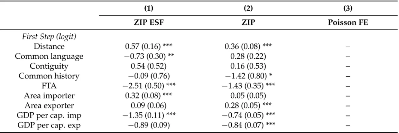
Table A1.Estimated coefficients for: (1) ZIP ESF; (2) ZIP; (3) Poisson FE.
(1) (2) (3)
ZIP ESF ZIP Poisson FE
First Step (logit)
Distance 0.57 (0.16) *** 0.36 (0.08) *** – Common language −0.73 (0.30) ** 0.28 (0.22) – Contiguity 0.54 (0.52) 0.16 (0.53) – Common history −0.09 (0.76) −1.42 (0.80) * – FTA −2.51 (0.50) *** −1.43 (0.35) *** – Area importer 0.32 (0.08) *** 0.05 (0.05) – Area exporter 0.09 (0.06) 0.28 (0.05) *** –
GDP per cap. imp −1.35 (0.11) *** −0.74 (0.05) *** –
Table A1. Cont.
(1) (2) (3)
ZIP ESF ZIP Poisson FE
Population imp −1.02 (0.12) *** −0.45 (0.08) *** – Population exp −1.01 (0.10) *** −1.16 (0.08) *** – Island imp −0.48 (0.64) −1.16 (0.41) *** – Island exp 0.44 (0.54) −1.73 (0.47) *** – Landlocked imp 3.74 (0.48) *** −0.14 (0.18) – Landlocked exp −0.15 (0.31) −1.06 (0.22) *** – Constant 38.69 (3.27) *** 31.10 (2.30) *** – Eigenvectors (exp) 10 – – Eigenvectors (imp) 16 – – Eigenvectors (network) 28 – –
Second Step (Poisson)
Distance −0.58 (0.04) *** −0.39 (0.04) *** −0.62 (0.03) *** Common language 0.09 (0.08) 0.40 (0.11) *** 0.10 (0.07) Contiguity 0.56 (0.10) *** 0.66 (0.15) *** 0.58 (0.07) *** Common history 0.19 (0.09) ** 0.13 (0.10) 0.06 (0.08) FTA 0.45 (0.08) *** 0.72 (0.08) *** 0.44 (0.06) *** Area imp −0.19 (0.02) *** −0.07 (0.02) *** −0.26 (0.14) * Area exp −0.003 (0.02) −0.05 (0.02) ** 0.37 (0.16) ** GDP per cap. imp 0.77 (0.03) *** 0.80 (0.03) *** 0.77 (0.14) ** GDP per cap. exp 0.77 (0.02) *** 0.67 (0.03) *** 0.92 (0.23)
Population imp 0.91 (0.03) *** 0.84 (0.02) *** 1.44 (0.14) *** Population exp 0.73 (0.03) *** 0.76 (0.03) *** 0.29 (0.26) Island imp −0.03 (0.07) −0.13 (0.08) * −0.47 (0.43) Island exp −0.49 (0.08) *** −0.23 (0.08) *** 0.30 (0.63) Landlocked imp 0.002 (0.10) −0.05 (0.10) 0.50 (0.76) Landlocked exp 0.14 (0.10) −0.19 (0.12) 0.09 (1.27) Constant −28.48 (0.71) *** −29.52 (0.91) *** −35.32 (3.71) *** Eigenvectors (exp) 6 – – Eigenvectors (imp) 7 – – Eigenvectors (network) 24 – –
Fixed Effects (exp) No No Yes
Fixed Effects (imp) No No Yes
AIC 1,477,400 2,545,233 1,467,313
Log-likelihood −738,577 −1,272,584 −733,525
McFadden’s pseudo-R2 0.935 0.888 0.935
Observations 4032 4032 4032
Residual dof 3910 4000 3872
***, **, * denote statistical significance at the 1, 5, 10 per cent level. Standard errors in parenthesis.
Table A2.Counts of observed versus predicted values.
Trade Flow
(in US$ Millions, Rounded) 0 1 2 3 4 5 6 7 8 9
Observed 484 136 112 76 64 39 42 49 35 29
ZIP ESF 485 8 12 15 18 19 20 20 20 20
ZIP 484 0 1 1 2 3 4 5 6 7
References
Anderson, James E. 1979. A theoretical foundation for the gravity equation. The American Economic Review 69: 106–16.
Anderson, James E., and Eric van Wincoop. 2003. Gravity with gravitas: A solution to the border puzzle. American Economic Review 93: 170–92. [CrossRef]
Anderson, James E., and Eric van Wincoop. 2004. Trade costs. Journal of Economic Literature 42: 691–751. [CrossRef] Baier, Scott L., and Jeffrey H. Bergstrand. 2009. Bonus vetus OLS: A simple method for approximating international
trade-cost effects using the gravity equation. Journal of International Economics 77: 77–85. [CrossRef] Baltagi, Badi H., and Petter Egger. 2016. Estimation of structural gravity quantile regression models. Empirical
Economics 50: 5–15. [CrossRef]
Baltagi, Badi H., Peter Egger, and Michael Pfaffermayr. 2007. Estimating models of complex FDI: Are there third-country effects? Journal of Econometrics 140: 260–81. [CrossRef]
Behrens, Kristian, Cem Ertur, and Wilfried Koch. 2012. ‘Dual’ gravity: Using spatial econometrics to control for multilateral resistance. Journal of Applied Econometrics 25: 773–94. [CrossRef]
Burger, Martijn, Frank van Oort, and Gert-Jan Linders. 2009. On the specification of the gravity model of trade: Zeros, excess zeros and zero-inflated estimation. Spatial Economic Analysis 4: 167–90. [CrossRef]
Buu, Anne, Norman J. Johnson, Runze Li, and Xianming Tan. 2011. New variable selection methods for zero-inflated count data with applications to the substance abuse field. Statistics in Medicine 30: 2326–40. [CrossRef] [PubMed]
Chen, Tian, Pan Wu, Wan Tang, Hui Zhang, Changyong Feng, Jeanne Kowalski, and Xin M. Tu. 2016. Variable selection for distribution-free models for longitudinal zero-inflated count responses. Statistics in Medicine 35: 2770–85. [CrossRef] [PubMed]
Chun, Yongwan. 2008. Modeling network autocorrelation within migration flows by eigenvector spatial filtering. Journal of Geographical Systems 10: 317–44. [CrossRef]
Chun, Yongwan, and Daniel A. Griffith. 2011. Modeling network autocorrelation in space–time migration flow data: An eigenvector spatial filtering approach. Annals of the Association of American Geographers 101: 523–36. [CrossRef]
Chun, Yongwan, and Daniel A. Griffith. 2013. Spatial Statistics and Geostatistics: Theory and Applications for Geographic Information Science and Technology. London: Sage.
Chun, Yongwan, Daniel A. Griffith, Monghyeon Lee, and Parmanand Sinha. 2016. Eigenvector selection with stepwise regression techniques to construct eigenvector spatial filters. Journal of Geographical Systems 18: 67–85. [CrossRef]
Cliff, Andrew David, and J. K. Ord. 1981. Spatial Processes: Models & Applications. London: Pion.
Cliff, Andrew, and Keith Ord. 1972. Testing for spatial autocorrelation among regression residuals. Geographical Analysis 4: 267–84. [CrossRef]
Curry, L. 1972. A spatial analysis of gravity flows. Regional Studies 6: 131–47. [CrossRef]
Curry, Leslie, Daniel A. Griffith, and Eric S. Sheppard. 1975. Those gravity parameters again. Regional Studies 9: 289–96. [CrossRef]
Efroymson, M. A. 1960. Multiple regression analysis. In Mathematical Methods for Digital Computers. Edited by Ralston, Anthony and Herbert S. Wilf. New York: Wiley, pp. 191–203.
Egger, Peter H., and Kevin E. Staub. 2016. GLM estimation of trade gravity models with fixed effects. Empirical Economics 50: 137–75. [CrossRef]
Egger, Peter H., and Filip Tarlea. 2015. Multi-way clustering estimation of standard errors in gravity models. Economics Letters 134: 144–47. [CrossRef]
Feenstra, Robert C., Robert E. Lipsey, Haiyan Deng, Alyson C. Ma, and Hengyong Mo. 2005. World Trade Flows: 1962–2000. NBER Working paper No. 11040, National Bureau of Economic Research, Cambridge, MA, USA. Fischer, Manfred M., and Daniel A. Griffith. 2008. Modeling spatial autocorrelation in spatial interaction data: An application to patent citation data in the european union. Journal of Regional Science 48: 969–89. [CrossRef] Flowerdew, Robin, and Murray Aitkin. 1982. A method of fitting the gravity model based on the poisson
distribution. Journal of Regional Science 22: 191–202. [CrossRef] [PubMed]
Gilles, Rodica, and Seik Kim. 2017. Distribution-free estimation of zero-inflated models with unobserved heterogeneity. Statistical Methods in Medical Research 26: 1532–42. [CrossRef] [PubMed]
Greene, William H. 1994. Accounting for Excess Zeros and Sample Selection in Poisson and Negative Binomial Regression Models. NYU working paper No. EC-94-10, New York University, New York, NY, USA. Griffith, Daniel A. 2003. Spatial Autocorrelation and Spatial Filtering: Gaining Understanding through Theory and
Scientific Visualization. Berlin, Heidelberg, and New York: Springer-Verlag.
Griffith, Daniel A. 2007. Spatial structure and spatial interaction: 25 years later. The Review of Regional Studies 37: 28–38.
Griffith, Daniel A. 2009. Spatial autocorrelation in spatial interaction: Complexity-to-simplicity in journey-to-work flows. In Complexity and Spatial Networks: In Search of Simplicity. Edited by Reggiani, Aura and Peter Nijkamp. Berlin and Heidelberg: Springer-Verlag, pp. 221–37.
Griffith, Daniel A., and Yongwan Chun. 2016. Evaluating eigenvector spatial filter corrections for omitted georeferenced variables. Econometrics 4: 29. [CrossRef]
Head, Keith, and Thierry Mayer. 2014. Chapter 3—Gravity equations: Workhorse, toolkit, and cookbook. In Handbook of International Economics. Edited by Gopinath, Gita, Elhanan Helpman and Kenneth Rogoff. Amsterdam and Oxford: Elsevier, vol. 4, pp. 131–95.
Helpman, Elhanan, Marc Melitz, and Yona Rubinstein. 2008. Estimating trade flows: Trading partners and trading volumes. The Quarterly Journal of Economics 123: 441–87. [CrossRef]
Jansen, Marion, and Hildegunn Kyvik Nordås. 2004. Institutions, Trade Policy and Trade Flows. CEPR discussiong paper No. 4418, Centre for Economic Policy Research, Lodon, UK.
Kitazawa, Yoshitsugu. 2014. Consistent Estimation for the Full-Fledged Fixed Effects Zero-Inflated Poisson Model. Discussion paper No. 66, Faculty of Economics, Kyushu Sangyo University, Fukuoka, Japan.
Koch, Wilfried, and James P. LeSage. 2015. Latent multilateral trade resistance indices: Theory and evidence. Scottish Journal of Political Economy 62: 264–90. [CrossRef]
Krisztin, Tamás, and Manfred M. Fischer. 2015. The gravity model for international trade: Specification and estimation issues. Spatial Economic Analysis 10: 451–70. [CrossRef]
Lambert, Diane. 1992. Zero-inflated poisson regression, with an application to defects in manufacturing. Technometrics 34: 1–14. [CrossRef]
Lambert, Dayton M., Jason P. Brown, and Raymond J.G.M. Florax. 2010. A two-step estimator for a spatial lag model of counts: Theory, small sample performance and an application. Regional Science and Urban Economics 40: 241–52. [CrossRef]
LeSage, James P., and Manfred M. Fischer. 2016. Spatial regression-based model specifications for exogenous and endogenous spatial interaction. In Spatial Econometric Interaction Modelling. Edited by Patuelli, Roberto and Giuseppe Arbia. Heidelberg and Berlin: Springer.
LeSage, James P., and R. Kelley Pace. 2008. Spatial econometric modeling of origin-destination flows. Journal of Regional Science 48: 941–67. [CrossRef]
Leung, Siu Fai, and Shihti Yu. 1996. On the choice between sample selection and two-part models. Journal of Econometrics 72: 197–229. [CrossRef]
Linders, Gert-Jan M., Martijn J. Burger, and Frank G. van Oort. 2008. A rather empty world: The many faces of distance and the persistent resistance to international trade. Cambridge Journal of Regions, Economy and Society 1: 439–58. [CrossRef]
Long, J. Scott. 1997. Regression Models for Categorical And Limited Dependent Variables. Thousand Oaks: Sage Publications. Majo, M.C., and A. van Soest. 2011. The fixed-effects zero-inflated poisson model with an application to health care utilization. CentER Working Paper No. 2011–083, CentER, Tilburg University, Tilburg, The Netherlands. Martin, William J., and Cong S. Pham. 2015. Estimating the Gravity Model When Zero Trade Flows Are Frequent and Economically Determined. Policy Research working paper No. WPS 7308, World Bank Group, Washington, DC, USA.
Martínez-Zarzoso, Inmaculada. 2013. The log of gravity revisited. Applied Economics 45: 311–27. [CrossRef] Nordås, Hildegunn Kyvik. 2008. Gatekeepers to consumer markets: The role of retailers in international trade.
The International Review of Retail, Distribution and Consumer Research 18: 449–72. [CrossRef]
Papadopoulos, Georgios, and J.M.C Santos Silva. 2012. Identification issues in some double-index models for non-negative data. Economics Letters 117: 365–67. [CrossRef]
Patuelli, Roberto, Norbert Schanne, Daniel A. Griffith, and Peter Nijkamp. 2012. Persistence of regional unemployment: Application of a spatial filtering approach to local labour markets in germany. Journal of Regional Science 52: 300–23. [CrossRef]
Patuelli, Roberto, Gert-Jan M. Linders, Rodolfo Metulini, and Daniel A. Griffith. 2016. The space of gravity: Spatially filtered estimation of a gravity model for bilateral trade. In Spatial Econometric Interaction Modelling. Edited by Patuelli, Roberto and Giuseppe Arbia. Cham: Springer International Publishing, pp. 145–69. Philippidis, George, Helena Resano-Ezcaray, and Ana I. Sanjuán-López. 2013. Capturing zero-trade values in
gravity equations of trade: An analysis of protectionism in agro-food sectors. Agricultural Economics 44: 141–59. [CrossRef]
Preisser, John S., John W. Stamm, D. Leann Long, and Megan E. Kincade. 2012. Review and recommendations for zero-inflated count regression modeling of dental caries indices in epidemiological studies. Caries Research 46: 413–23. [CrossRef] [PubMed]
Santos Silva, João M.C., and Silvana Tenreyro. 2006. The log of gravity. Review of Economics and Statistics 88: 641–58. [CrossRef]
Santos Silva, J.M.C., and Silvana Tenreyro. 2011. Further simulation evidence on the performance of the poisson pseudo-maximum likelihood estimator. Economics Letters 112: 220–22. [CrossRef]
Scherngell, Thomas, and Rafael Lata. 2013. Towards an integrated european research area? Findings from eigenvector spatially filtered spatial interaction models using european framework programme data. Papers in Regional Science 92: 555–77. [CrossRef]
Sellner, Richard, Manfred Fischer, and Matthias Koch. 2013. A spatial autoregressive poisson gravity model. Geographical Analysis 45: 180–201. [CrossRef]
Sheppard, Eric S., Daniel A. Griffith, and Leslie Curry. 1976. A final comment on mis-specification and autocorrelation in those gravity parameters. Regional Studies 10: 337–39. [CrossRef]
Wang, Zhu, Shuangge Ma, and Ching-Yun Wang. 2015. Variable selection for zero-inflated and overdispersed data with application to health care demand in germany. Biometrical Journal 57: 867–84. [CrossRef] [PubMed] Xiong, Bo, and John Beghin. 2012. Does european aflatoxin regulation hurt groundnut exporters from africa?
European Review of Agricultural Economics 39: 589–609. [CrossRef]
Zeng, Ping, Yongyue Wei, Yang Zhao, Jin Liu, Liya Liu, Ruyang Zhang, Jianwei Gou, Shuiping Huang, and Feng Chen. 2014. Variable selection approach for zero-inflated count data via adaptive lasso. Journal of Applied Statistics 41: 879–94. [CrossRef]
© 2018 by the authors. Licensee MDPI, Basel, Switzerland. This article is an open access article distributed under the terms and conditions of the Creative Commons Attribution (CC BY) license (http://creativecommons.org/licenses/by/4.0/).