Sustainable managment of stormwater in a changing environment under Mediterranean climate conditions

(1)

DOTTORATO DI RICERCA IN “RISCHIO E SOSTENIBILITA' NEI SISTEMI DELL'INGEGNERIA CIVILE, EDILE E AMBIENTALE”

XXX Ciclo - Nuova Serie (2014-2017)

DIPARTIMENTO DI INGEGNERIA CIVILE,UNIVERSITÀ DEGLI STUDI DI SALERNO

SUSTAINABLE MANAGEMENT OF

STORMWATER IN A CHANGING

ENVIRONMENT UNDER

MEDITERRANEAN CLIMATE CONDITIONS

ING.(DOTT.)MIRKA MOBILIA

Relatore:

PROF. ING.ANTONIA LONGOBARDI

Coordinatore

(2)

(3)

SUSTAINABLE MANAGMENT OF STORMWATER IN A CHANGING ENVIRONMENT UNDER MEDITERRANEAN CLIMATE CONDITIONS __________________________________________________________________ Copyright © 2005 Università degli Studi di Salerno – via Ponte don Melillo, 1 – 84084 Fisciano (SA), Italy – web: www.unisa.it

All rights reserved. No part of this publication may be reproduced, distributed, or transmitted in any form or by any means, including photocopying, recording, or other electronic or mechanical methods, without the prior written permission of the publisher. Although the author have paid the maximum attention in writing the present manuscript, he accepts no responsibility for inaccuracies or omissions. The author assumes no responsibility for any complications of any kind that may be incurred by the reader as a result of actions arising from the use and application of the contents of this manuscript.

(4)

(5)

LIST OF FIGURES

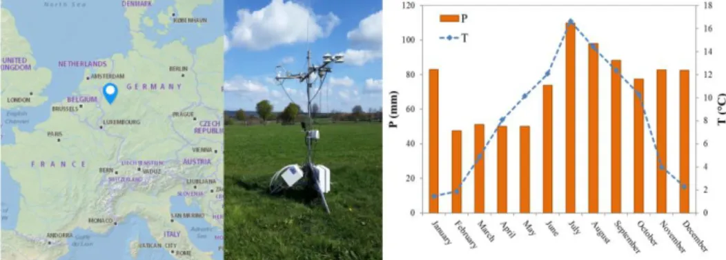
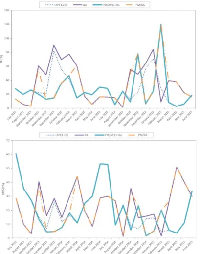
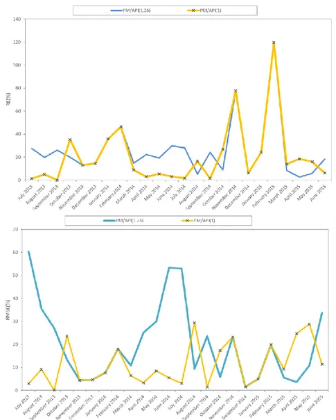
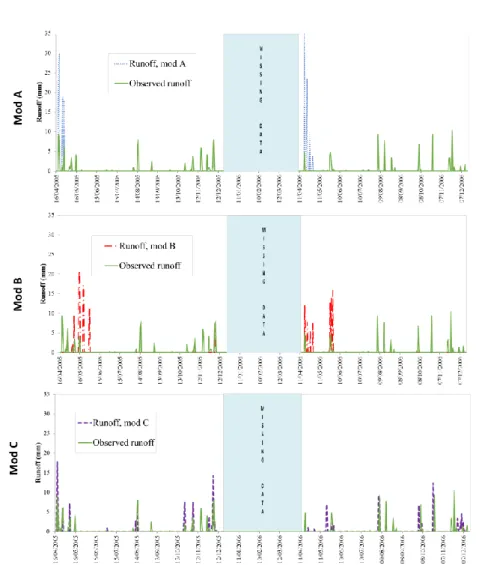
Figure 3.1 Location of the Rollesbroich grassland site in Germany (left) and the Eddy covariance station (right) at the site. ... 21 Figure 3.2 Monthly patterns for precipitation (P), eddy covariance actual evapotranspiration (AETec), Penman-Montheith potential evapotranspiration (PETpm) and Budyko aridity index (P/PET). The dotted line P/PET = 1 represents the threshold limit between energy limited and water limited systems. ... 26 Figure 3.3 Monthly patterns for eddy covariance actual evapotranspiration (AETec), Penman-Montheith potential evapotranspiration (PETpm) and net radiation (Rn)... 27 Figure 3.4 Monthly values of RE and RMSE for the proposed models. 30 Figure 3.5 Calibrated monthly values of the Priestly Taylor coefficient . ... 31 Figure 3.6 Monthly values of RE and RMSE for PM/API(1.26) and PM/API(1). ... 32 Figure 4.1 Green roof location and composition. ... 34 Figure 4.2 Patterns of mean monthly rain and temperature for the study site. ... 35 Figure 4.3 Water depth (V) and water holding capacity (W) daily scale patterns as a ratio to soil depth. Actual evapotranspiration losses are computed by the API Method. Overlapped, in the upper right corner, the scatter plot for the two considered variables and the relevant Person correlation coefficient. ... 38 Figure 4.4 Precipitation, antecedent precipitation index (API), air temperature, wind speed, radiation daily pattern for the experimental site. ... 42 Figure 4.5 Monthly patterns of PET and AET during the period of observation. ... 42 Figure 4.6 Comparison between modelled and observed runoff time series for the different approaches... 44 Figure 4.7 Comparison between cumulated observed runoff from the studied green roof and cumulated runoff modelled using the three

(8)

approaches with increasing level of complexity. a) simulated period:

2005. b) simulated period: 2006. ... 45

Figure 4.8 Impact of water holding capacity (as a percentage of soil total depth) for mod A (upper panel) and mod B (lower panel). ... 48

Figure 5.1 Green roofs Experimental site in Salerno . ... 50

Figure 5.2 Plans and sections of the benches. ... 51

Figure 5.3 Drainage layer with clay and commercial panel filled with clay). ... 52

Figure 5.4 Weather monitoring systems ... 52

Figure 5.5 Seasonal patterns of rain for Salerno and Trier. ... 53

Figure 5.6 Irrigation system for GR1 and GR2 ... 54

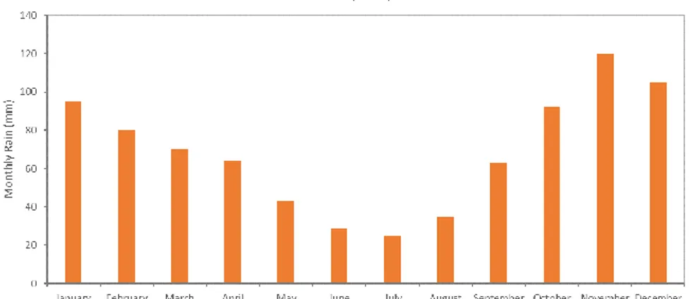
Figure 5.7 Monthly values of rain for the experimental site ... 55

Figure 5.8 Temporal evolution of two rainfall events ………58

Figure 5.9 Retention capacity of two green roofs vs cumulative rainfall depth ... 62

Figure 5.10 Retention capacity of two green roofs vs duration of storm events ... 62

Figure 5.11 left panel-Retention capacity of two green roofs vs intensity of the real events, right panel- Retention capacity of two green roofs vs intensity of the simulated events ... 62

Figure 6.1 Basins sketched like non linear reservoirs. ... 65

Figure 6.2 Vertical layers of SUDS infrastructures. ... 68

Figure 6.3 Parameters used in the flows balance equations. ... 69

Figure 6.4 The virtual basin. ... 72

Figure 6.5 IDF curves. ... 72

Figure 6.6 Homogeneous rainfall areas in Campania. ... 75

Figure 6.7 Synthetic hyetographs for duration of 1, 3, 24 hours... 80

Figure 6.8 Performances in terms of ΔRV, ΔPF, ΔDT varying the percentage of retrofitting... 83

Figure 6.9 Virtual basin with 8 sub-catchment. ... 85

Figure 6.10 Virtual basin with 16 sub-catchment. ... 86

Figure 7.1 Baronissi rain gauge station change point detection test. Left panel: U-test. Right panel: t-test. ... 93

Figure 7.2 Baronissi rain gauge station change point detection test. Upper panel: Pettitt’s test. Lower panel: CUMSUM test. ... 94

Figure 7.3 Maximum annual 24 h rainfall time series for the four investigated rain gauge stations. ... 100

(9)

Figure 7.4 Site locations where MDHE have been recorded during last 60 years. Blue lines indicate main streams and red circles flooded areas

(most frequent occurrences). ... 101

Figure 7.5 Documentary photos. ... 101

Figure 7.6 The area under investigation and the rain gauges network. Yellow squares: site locations where MDHE have been recorded during last 60 years. Red circles: historical rain gauge stations. Magenta circles: rain gauge station installed after 2000. Blue lines: main streams network. ... 104

Figure 7.7 Temporal distribution and characterization of occurred MDHE in the Solofrana river basin. ... 104

Figure 7.8 MDHEs BSC types most frequently occurring within the Solofrana river basin. Left panel represent BSC for the 19/09/2011 event. Right panel represent BSC for the 08/10/2013 event. ... 105

Figure 7.9 Process for the elaboration of SAR images. ... 109

Figure 7.10 The clustering-based thresholding images of Sarno river basin. ... 112

Figure 7.11 Evolution of build-up area in time. ... 113

Figure 7.12 The area under investigation... 114

Figure 7.13 Sub-catchments, trunks and nodes of Sarno river basin... 115

Figure 7.14 Sarno river basin in SWMM. ... 116

Figure 7.15 Conduit’s cross section geometry (in centimeters) for each section where the main river joins its tributaries. ... 118

Figure 7.16 Synthetic hyetographs for duration of 10 hours. ... 120

Figure 7.17 Flooded sections and flooding volume before (left panel) and after (right panel) the retrofitting, occurring for design storm events ... 121

Figure 7.18 Characteristics of the studied rainfall event. ... 123

Figure 7.19 Rainfall records from 3 rain gauge stations in Sarno basin. ... 123

Figure 7.20 Thiessen polygons for the basin under investigation. ... 124

Figure 7.21 Flooded sections and flooding volume before (left panel) and after (right panel) the retrofitting, occurring for the actual event. ... 125

Figure 7.22 The urban drainage system of Preturo... 125

Figure 7.23 Urban drainage system of Preturo in SWMM. ... 126

Figure 7.24 Buildings selected according to the number of stories. ... 129

Figure 7.25 Buildings selected according to the orientation of the roof. ... 129

Figure 7.26 Buildings selected according to the number of site boundaries. ... 130

(10)

Figure 7.27 Areas selected according for the replacement with Permeable Pavements. ... 133

(11)

LIST OF TABLES

Table 3.1 Global values of the goodness-of-fit indices for the proposed

models. ... 29

Table 4.1 Models settings for different model complexity level. Mod A represents the basic approach. Mod B represents the intermediate approach. Mod C represents the advanced approach. ... 36

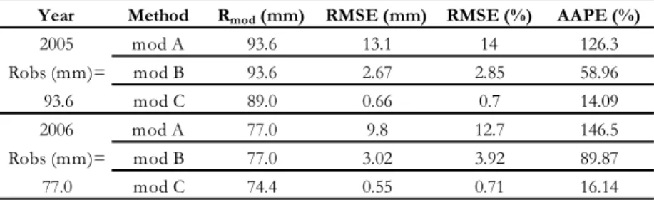
Table 4.2 Values of the RMSE and AAPE for the different approaches. ... 46

Table 4.3 Calibrated (mod A and mod B) and average (mod C) maximum water holding capacities as percentage of total soil depth. ... 46

Table 5.1 Parameters used for the calculation of irrigation water need . 57 Table 5.2 Real and simulated events ... 61

Table 6.1 Combination of layers for each SUDS technique. ... 70

Table 6.2 Parameters used for Bio-retention cells. ... 71

Table 6.3 Values required for the design. ... 75

Table 6.4 Flows in the pipes. ... 75

Table 6.5 Average slope of the water route... 77

Table 6.6 Intercept and the slope of the IDF curves. ... 79

Table 6.7 GR response varying the percentages of retrofitted roofs. ... 82

Table 6.8 GR response varying the spatial GRs distribution in the basin. ... 84

Table 6.9 Effect of spatial scale of aggregation on GRs response (8 sub-basins). ... 85

Table 6.10 Effect of spatial scale of aggregation on GRs response (16 sub-basins)... 87

Table 7.1 Rain gauge stations metadata indications. ... 89

Table 7.2 Change point detection analysis results (significance level 10%). Indication of change points occurrence year is also given. ... 94

Table 7.3 Baronissi rain gauge station trend detection analysis results. .. 99

Table 7.4 Forino rain gauge station trend detection analysis results... 99

Table 7.5 Mercato San Severino rain gauge station trend detection analysis results. ... 100

Table 7.6 Serino rain gauge station trend detection analysis results. ... 100 Table 7.7 MDHEs inventory for the Solofrana peri-urban catchment. 102

(12)

Table 7.8 Parameters for the homogeneous areas. ... 106

Table 7.9 MDHEs and main rainfall characteristics. ... 108

Table 7.10 Soil consuption Assessment (%) related to the geographical areas. Source:ISPRA-ARPA-APPA monitoring network. ... 109

Table 7.11 Characteristics of the two sensors. ... 110

Table 7.12 The two sets of SAR images. ... 110

Table 7.13 Built-up area in each sub-basin. ... 112

Table 7.14 Coordinates of the study area. ... 114

Table 7.15 The main properties of the sub-catchments, trunks and nodes of Sarno river basin. ... 117

Table 7.16 SCS Runoff Curve Numbers (Antecedent moisture condition II). ... 119

Table 7.17 Seasonal rainfall limits for AMC. ... 120

Table 7.18 Percentage of reduction of flooded sections and flooding volume occurring for design storm events in Sarno basin. ... 121

Table 7.19 List of rain gauges in the Sarno river basin. ... 122

Table 7.20 Percentage of reduction of flooded sections and flooding volume occurring for actual event in Sarno basin. ... 124

Table 7.21 The main properties of the sub-catchments, trunks and nodes of Preturo district. ... 127

Table 7.22 Percentages of green roof retrofit potential in each basin. .. 131

Table 7.23 Percentage of reduction of flooded sections and flooding volume occurring using GRs for actual event in Preturo district. ... 131

Table 7.24 Percentage of potential use of permeable pavements in Preturo district. ... 132

Table 7.25 Percentage of reduction of flooded sections and flooding volume occurring using GRs and Permeable Pavements for actual event in Preturo district. ... 133

(13)

ABSTRACT

The problem of the increase in the magnitude and frequency of flooding events in urban areas can be approached by means of techniques of sustainable urban stormwater management. In this PhD dissertation, the effectiveness of one of these technologies namely the green roof (GR), has been investigated. For this purpose, a daily scale hydrological model for GRs, mainly based on meteorological data and with three levels of complexity has been proposed. Since, the evapotranspiration (ET) fluxes impact the GR retention performances, a study of the dynamics involved in ET process has been carried out. The use of green roofs technology in Mediterranean climate is very limited so two GR experimental benches has been placed in the campus of University of Salerno and preliminary results about the hydrological performances depending on the climate and constructions characteristics have been illustrated. Subsequently, the effectiveness of the proposed technology for the sustainable urban drainage management have been tested at a large scale and Sarno peri-urban basin has been presented as case study since it represents a hydrogeological hazard prone system. The analysis focused on the potential hydrological benefits in terms of peak runoff, peak delay and volume runoff in respect of several hypothetical scenarios of rainfall and GR retrofitting percentage. In high urbanized areas, the implementation of GRs at basin scale, allows a reduction of runoff rainwater from roofs close to 100% for some rainfall and greening scenarios. Where the GR retrofit potential is very low, satisfactory performances in terms of water management can be reached coupling this green technology to other sustainable techniques.

(14)

ABOUT THE AUTHOR

Mirka Mobilia Ing. Mirka Mobilia earned a Bachelor's degree in

Environmental Engineering at University of Salerno in 2011. In 2014 she earned Master's degree in Environmental Engineering, at University of Salerno. In November 2014,she started a Ph.D. course in “Risk and sustainability in civil, environmental and construction engineering”, at the Civil Engineering Department ,University of Salerno. Her research interest is about the sustainable stormwater management for urban drainage systems, with a particular focus on urban greening. During her studies, she spent three research periods abroad at the University of Applied Sciences of Trier, at the Technical University of Darmstadt and at the Institute of Bio- and Geosciences (Forschungszentrum) of Jülich, where she had the opportunity to deepen her knowledge about experimental site monitoring and hydrological modelling.

(15)

1 INTRODUCTION

Many cities around the world are increasingly called to deal with the two major challenges of climate change and urbanization. Both of them cause an increase in the magnitude and frequency of flooding in urban areas. In order to face these criticisms, adaptation measures are required for conventional drainage systems with limited capacity and flexibility. They help the urban drainage infrastructures to improve their resilience against the adverse impact of climate change and rapid urbanization in a context where reducing risk of flooding becomes more and more urgent. Among adaptations approaches, techniques of sustainable urban stormwater management like Green infrastructures (GIs) represent a very attractive issue because of the variety of benefits, beyond the hydrological perspective, they can provide for urban environments. They are conceived as a network of greenspaces around urban landscapes providing environmental, social and economic benefits to the community indeed. Among these the green roofs (GRs) technique are an effective tool for pursuing the concept of a sustainable stormwater management. The technology of green roofs induces important hydraulic benefits compared to a traditional roof, such as decrease in runoff volume, peak discharge attenuation and increase in the peak delay. With reference to the hydrological issue related to GIs application within the European geographical context, the sustainable urban drainage management has been widely implemented in the Nordic countries characterized by oceanic climate with warm summers and cool winters and a negligible seasonal pattern. In these regions, the hydrological performances of the green techniques in terms of retention capacity have been investigated in detail and many contributions exist in the specific literature from which it appears that their behavior is not yet fully understood because affected by multiple factors like the types of rainfall event, the climate condition of the study area and the construction type of the roof. In the Mediterranean climate, the uncertainty in GIs hydrological performances is even more evident because of the marked climate stress and differences between the seasons and because of a limited number of test beds providing experimental data. In light of this,

(16)

the reported research work has contributed to the understanding of this question with the proposal of a conceptual model strongly grounded on the meteorological conditions for an accurate prediction of green roofs’ hydrological behavior at the building scale and with the setup of an experimental site located within the University of Salerno campus. With a particulr focus on a mediterranean catchment characterized by evolving climate and land use conditions, the main aim of the present thesis is the investigation of the sensitivity of the cathment stormwter response to the use of green infrastructures, as a valid tool for the mitigation of hydrogeological risk in urban and peri-urban environments.

In this respect, after a review of the state of the art set out in the chapter 2 of the present work, in the chapter 3, a study of the evapotranspiration dynamics that is a key process affecting the hydrological behavior of green roofs, has been carried out. In the chapter 4, as a result of a modeling with increasing levels of complexity, a daily scale hydrological model for GRs, mainly based on meteorological data, has been proposed. Finally, in the chapter 5, the GR experimental site located in the campus of University of Salerno has been illustrated and preliminary results about the hydrological performances depending on the climate and constructions characteristics have been shown.

In the second part of the thesis, arguing about the limits of a traditional urban drainage system management model where urban flooding prevention is achieved with the use of centralized strategies, generally corresponding to underground concrete tanks connected to the main drainage network, the effectiveness of the proposed technologies for the sustainable urban drainage management have been tested at a large scale. As already said, because of the lack of experimental sites in Italy, especially for what concerns the catchment scale, the research work has been mainly focused on a sensitivity analysis aiming at verify the potential improvement related to the use of GI, from the hydrological point of view. The case study is represented by the Sarno peri-urban basin (Campania region), selected as it represent a hydrogeological hazard prone system and is characterized by an extremely fragile equilibrium at the urban level.

Pursuing this line, in the chapters 6 and 7, the analysis of the hydrological performances of green roof at basin scale in terms of peak runoff, peak delay and volume runoff, has been performed. The susceptibility of the hydrological response to spatial distribution, scale of aggregation and percentage of retrofitted roofs has been tested. A wide

(17)

range of situations have been simulated from scenarios related to virtual basin and design storms to scenarios referring to actual catchment and real events occurred in the past. Finally, the analysis investigates the impacts of the sustainable urban stormwater management infrastructures at the basin scale and the potential for such infrastructures to be effectively and diffusely accounted for in planning and managing the urban environment on the way for a sustainable environment.

(18)

2 STATE OF ART

Many cities around the world are increasingly called to deal with the two major challenges of climate change and urbanization (Zhou 2014). Both of them cause an increase in the magnitude and frequency of flooding in urban areas (Huong et al. 2013, Leopold 1968, Semadeni-Davies et al. 2008, Zhou et al. 2012). According to several scholars (Willems et al. 2012, Arnbjerg-Nielsen et al. 2012, Ekström et al. 2005), the climate change could address in the coming years more frequent rain of increased peak intensity leading inevitably to more sewer floods because of the overloading of the urban drainage systems, designed with a certain return period. The urbanization has same impacts on sewer infrastructure as climate change. The United Nations (UN, 2014) predict that, the world’s population will increase between 1950 and 2100 of about 9 billion people with more than 66% living in urban areas. The increase in urban population involves a sprawl sealing surfaces including industrial commercial and residential settlements. In cities with extensive impermeable areas, the amount of occurring runoff is higher than in case of low urbanization and consequently the risk of flooding increases too (Huong et al. 2013). The dynamic of urbanization can be monitored with SAR images guaranteeing observations and measurements at high spatial and temporal resolution (Taubenböck, et al. 2012, Ban et al. 2012). SAR images acquired over the same area at different times allow to map the process of urbanization in time, and comparing this data with a database of urban flooding events, the identification of a relationship between the occurrences of flooding and the land use changes could be possible. In time many authors have used the SAR images for different research purposes (Di Martire et al. 2016, Weijie et al. 2015, Zhu et al. 2016 ). Some authors have used this kind of images to investigate the spatial evolution of urbanization (Ban et al. 2012, Zhu et al. 2012, Fu et al. 2014, Ma et al. 2014), few of them have used Synthetic aperture radar images for hydraulic aims (Haas et al. 2014, Dewan et al. 2008). In order to face the criticism of flooding in urban areas, adaptation measures are required for conventional drainage systems with limited capacity and flexibility (Jha et al. 2011). They help the urban sewer infrastructures to improve their resilience against the adverse impact of climate change and

(19)

rapid urbanization in a context where reducing risk of flooding becomes even more urgent. The adaptations options include techniques of sustainable management of urban stormwater known around the world with different denominations but with similar principles. In North America and New Zealand, the term LID or low impact development is used to indicated a variety of practices that mimic natural processes in the management of stormwater (Fletcher et al. 2015). In United States and Canada, BMP (Best management practices) refers to practices aiming to prevent pollution (Fletcher et al. 2015). In UK and in general in Europe, sustainable urban drainage systems (SUDS) consist of technologies able to drain rainwater as closely as possible to the natural drainage from a site before development (Woods-Ballard et al. 2007). Green infrastructures (GIs) are an integral part of SUDS (Mguni et al. 2016). They are conceived as a network of greenspaces around urban landscapes providing environmental, social and economic benefits to the community (Benedict et al. 2002, Sartor et al. 2018). GIs exactly fit, in terms of water management and urban flooding prevention, within the philosophy of SUDs, because they aim to provide a hydrological/drainage network being complementary and linking green space with built infrastructure (Ahern 2007). These techniques include green roofs, filter drains and filter strips, permeable surfaces, swales( shallow drainage channels), infiltration trenches, detention basins (Woods-Ballard et al. 2007).

Among these, in a relatively recent past, many scientific studies have demonstrated the potential of green roofs (GRs) (Carter et al. 2006, Shaharuddin et al. 2011, Mobilia et al. 2015a,b) in pursuing the concept of a sustainable stormwater management. These technologies induce important hydraulic benefits compared to the conventional rooftop: decrease in runoff volume (VanWoert et al. 2005, Berndtsson 2010), peak discharge attenuation (Trinh et al. 2013, Fioretti et al. 2010) and increase in the peak delay (Gibler 2015, Stovin et al. 2015). With reference to the green roof retention properties, different authors have reported significantly different hydrological performances with reduction of the total volume of precipitation ranging from 40 to 90% (Mentens et al. 2006, Teemusk et al. 2007, Jarrett et al. 2006). The retention capacity of a GR is obviously a function of the system configuration (Stovin et al. 2012) but especially of the climate conditions of the area where the roof is placed. The hydrological effectiveness of the eco-roofs changes in different weather conditions, even if a complete picture of the situations

(20)

can’t be presented due to lack of experimental sites in some climatic regimes. For instance, in Europe, green roof infrastructures are mainly implemented in northern regions such as Germany, (Zimmer et al. 1997, Mentens et al. 2006), Sweden and Denmark (Villarreal et al. 2005, Bengtsson 2005, Locatelli et al. 2014), UK (Kasmin et al. 2010, Stovin et al. 201), Stovin et al. 2013) where their hydrological effectiveness is well documented in literature and their performances in term of peak flow and runoff volume reduction and peak time delay have been investigated in detail. The use of green roofs technology in Mediterranean climate is more limited. There are few experimental sites aiming mostly to monitor other aspects of the behavior of green roofs, in particular the thermal one. Consequently, the effects in terms of stormwater mitigation of GRs require additional investigations (Olivieri et al. 2013, Lazzarin et al. 2005, Fioretti et al. 2010 ).

Together with the system configuration and the climate conditions, the hydrological processes occurring also play an important role in the assessment of stormwater related benefits of green roofs and especially the evapotranspiration loss, as discussed in many recent works, because it directly impacts the green roof retention performances (Poë et al. 2015, Starry et al. 2016, Feitosa et al. 2016, Voyde et al. 2010). Evapotranspiration (ET) continuously restores the retention capacity of a storage system consequently it is the major component in the water balance of hydrological systems (McMahon et al. 2013) and the uncertainty in its assessment would propagate through the hydrological soil water balance (Abbaspour et al., 2015). Long term AET (Actual Evapotranspiration) measurements are complex and costly to be obtained, and even if observational data exists, methods to assess AET fluxes are time-consuming (Burba et al. 2010). For these reasons, many authors have proposed various approaches for indirect AET modeling (Mobilia et al 2016a). Under the Budyko framework AET is dominated either by precipitation P or by potential evapotranspiration PET (Budyko 1974). AET rates approach precipitation values in case of dry climates (water availability limited conditions) and potential evapotranspiration values in case of wet climates (energy limited conditions). Introducing the aridity index P/PET, water availability limited systems and energy limited systems are characterized respectively by P/PET < 1 and P/PET > 1. Beyond a long term characterization, water availability an energy limited conditions can alternate in time for a given system, as the results of the intra-annual variability of

(21)

climatological variables and thus in evapotranspiration rates, that switch from actual to potential rates (Ryu et al. 2008, Zhang et al. 2016). Opposed to more physically based methods, requiring soil physical properties and soil moisture and vegetation monitored data, actual evapotranspiration modeling can be performed through the use of a class of methods, simply based on routinely measured meteorological variables. Among these methods the Antecedent Precipitation Index (API) model, the Advection-Aridity (AA) model (Brutsaert et al. 1979), the Granger and Gray (GG) model (Granger et al. 1989), the CRAE model (Morton 1978), the modified advection aridity (MAA) model proposed by Otsuki et al. 1984 can be listed. Despite the large number of scientific contributions existing in the specific literature, there is still no a method for the assessment of actual evapotranspiration losses, starting from simple meteorological data and able to: i) identify the temporal switching between water availability and energy limited conditions, in order to recognize time period where the evapotranspiration losses are dominated by PET; ii) model the evapotranspiration losses seasonal pattern moving from potential to actual rates, respectively during energy limited and water availability limited conditions.

The GR hydrological behavior is modeled by soil water balance approaches and evapotranspiration loss plays an important role into retention modeling frameworks. In time, a broad range of models, conceptual or more physically based, oriented to the event or to the continuous time scale, suitable for single building or catchment scale, have been proposed by numerous authors (Berthier et al. 2010, Sherrard et al 2011, Stovin et al. 2013, Jim et al. 2012, Poë et al 2015, Hardin et al. 2012). Their implementation generally requires a high number of input parameters related to the soil hydraulic properties including textural class of the soil, residual soil water content, saturated soil water content, saturated hydraulic conductivity, or related to the water flow boundary condition, and the initial condition in terms of the pressure head or the water content (Hilten et al. 2008, Hakimdavara et al. 2014). Model implementation to predict the effectiveness of a planned green-roof installation in a particular area is mostly complex, due to the above-mentioned required data and parameters of the hydraulic system to be simulated, which are usually not readily available without laboratory or field experiments. It is well known indeed how model complexity affects model performances. Relatively simpler approach are frequently

(22)

preferred to over complex one as low calibration requirements are associated to a more robust parameters estimation (Burstza-Adamiak et al. 2013, Carson et al., 2015, Starry et al. 2016). In view of this, a conceptual model approach essentially using only few basic input parameters and weather data recorded by inexpensive monitoring installations in the area of interest is required as an answer to mentioned limitations. It should be taken into account that if the green infrastructures want to be used for the mitigation of urban flooding events, in addition to the complexity related to the understanding of their behavior at single building scale, efforts should be made to figure out how they perform at a larger scale. In the latter case, the corresponding experimental sites do not exist and the relative contributions refer to sensitivity analysis aiming at verifying the potential hydrological impacts (Masseroni et al. 2016, Versini et al. 2016, Zimmerman et al. 2016, Mobilia et al. 2018a). In this kind of study, a key role has been played by the analysis of the dynamics occurring in different climate conditions but also of the extent of implementation of this technology according to the characteristics of the existing urban built heritage.

(23)

3 EVALUATION OF METEOROLOGICAL

DATA BASED EVAPOTRANSPIRATION

MODELS

In a water balance, evapotranspiration represents the largest component and therefore, errors in estimating ET loss, assume great significance. The assessment of hydrological performances of green roof requires the quantification of evapotranspiration loss that plays a key role in reducing stormwater input because it directly acts on its moisture content, and thus on its ability to retain water after rainfall events. In order to measure evaporation fluxes, very sophisticated techniques can be used but they require more experimental data and instrumentation than are normally available. Given this premise, a methodology for actual evapotranspiration losses only based on meteorological data has been proposed. The approach is very simple to implement because the data required as input are commonly and directly measured in weather stations or can be derived with the help of direct or empirical relationships. To this aim micro-meteorological data at the Rollesbroich experimental site have been analyzed for a period of two years from July 2013 to June 2015. The analysis highlights a seasonal pattern in Budyko index so based on the observed seasonal switch between water-limited and energy-limited conditions, a threshold approach, combining potential evapotranspiration formulation and empirical actual evapotranspiration relationships, has been proposed and validated against eddy covariance assessment. Using several goodness of fit indices (RMSE, RE, MAE, NSE, d and r) the deviation between modeled and measured ET fluxes have been investigated. Penman-Montheith formulation has been considered for the potential evapotranspiration assessment and two different empirical relationships have been applied, namely the advection-aridity “AA” and the “API” non-potential Priestly-Taylor models, as empirical actual losses relationships. At the monthly scale, the lowest error occurs when the API method is used to mimic the water availability limited conditions but further significant improvements in the model can be achieved through the calibration of the

(24)

Priestly-Taylor advection coefficient. Because the model prediction of ET agreed well with the estimates obtained with the EC measurements, the approach can be considered well performing in the assessment of the actual evapotranspiration loss to be used in retention models of green roofs (Mobilia et al. 2018b).

3.1 A

REVIEW OF EVAPOTRANSPIRATION MODELS

3.1.1 Study area and data collection

The grassland study site of Rollesbroich (50°37’19”N, 6°18’15”E) is located in western Germany close to the Belgian border (Figure 3.1). The catchment has an area of 31 ha and its elevation increases from 474 to 518 m.a.s.l.. The annual mean precipitation and air temperature are respectively about 1033 mm and 7.7 °C (Qu et al. 2016). While the air temperature has a clearly visible seasonal pattern, with minimum and maximum values occurring respectively during the winter and summer seasons, the precipitation amount is substantially and uniformly distributed during the year (Figure 3.1).

The composition of the higher plant species at the site is typical for traditionally managed grassland of the Ranunculus repens–Alopecurus pratensis plant community with the major species of meadow foxtail (Alopecurus pratensis), perennial rye grass (Lolium perenne), rough meadow grass (Poa trivialis) and common sorrel (Rumex acetosa) (Borchard et al. 2015). All components of the water balance (e.g. precipitation, evapotranspiration, runoff, soil water content) are continuously monitored using state-of-the-art instrumentation installed in the center of the field, including weather stations, a micrometeorological station, weighable lysimeters, runoff gauges, cosmic-ray soil moisture sensors, a wireless sensor network that monitors soil temperature, and soil moisture and a 4-component net radiometer. For a detailed description of the site and measurement facilities please see Gebler et al. 2015 and Post et al. 2015. Latent heat flux was obtained by the eddy covariance (EC) technique for time intervals of 30 minutes. The EC post-processing software TK3.1 (Mauder et al. 2011) was used to calculate latent heat flux from the vertical wind velocity obtained by the sonic anemometer (CSAT3,

(25)

Campbell Scientific, Inc., Logan, USA) and water vapor density obtained by an infrared gas analyzer (LI7500, LI-COR Inc., Lincoln, NE, USA).

Figure 3.1 Location of the Rollesbroich grassland site in Germany (left) and the Eddy covariance station (right) at the site.

The processing and quality assurance of the EC data followed the corresponding TERENO strategy presented in Mauder et al. 2013. Actual evapotranspiration was calculated from the latent heat flux using:

water W L LH AET    (3-1) ) 000006 . 0 0016 . 0 36 . 2 8 . 2500 ( 10 3 T T2 T3 L_water          (3-2) where AET is actual evapotranspiration (mm−1_{), LH is latent heat flux}

(Wm−2_{), ρ}

w is water density (kg m−3), Lwater is latent heat of condensation of water in the temperature range from −25 to 40 ◦C (J kg−1_{), and T is air} temperature (◦C).

Since eddy covariance measurements are inevitably including gaps a standard gap-filling procedure was applied after Reichstein et al. 2005 to calculate the daily, monthly and annual sums actual evapotranspiration.

3.1.2 Complementary relationships for actual

(26)

Complementary relationship (CR) models were introduced by Bouchet 1963, and allow to directly model actual evapotranspiration using conventional meteorological data. These models argue about a mechanism of feedback between actual evapotranspiration (AET) and potential (PET) evapotranspiration rates under condition of minimum advection in a homogeneous area. In other words, in a condition of wet surface, actual evapotranspiration equals the potential one, according to:

WET PET

AET   _(3-3)

also expressed as:

WET PET AET 2 _(3-4) and finally: PET WET AET 2  _(3-5)

Where WET is the wet environment evapotranspiration. WET environment or equilibrium evaporation is the evaporation rate occurring when the surface is saturated and energy supply is constant. Equ. 3-3 states that an increase in AET corresponds to an equivalent decrease of PET because when the surface gets dry, a reduction of actual evapotranspiration occurs, it leads to a decrease in humidity and an increase in air temperature, as consequence, the PET increases too by equal amount.

Among well-known complementary relationships, one of the most broadly used approaches, the Advection Aridity model (Brutsaert et al. 1979), has been here selected to quantify actual evapotranspiration losses based on meteorological variables measurements. It considered that AET models require previous calculation of Priestley and Taylor (P-T) 1972 (eq. 3-6) and Penman (eq. 3-7) potential evapotranspiration fluxes PET





_      _      _n _soil T P R G PET    1 , (3-6)

(27)





_                    _n _soil _A M P R G E PET     1 , (3-7)

where Δ is the slope of the saturation vapor pressure–temperature curve (kPa °C−1_{) , given by the formula:}





2 3 . 237 4098    T e_s (3-8)

es is the saturation vapor pressure:

         3 . 237 27 . 17 exp 611 . 0 T T e_s (3-9) T is the air temperature (°C),  is the psychrometric constant (kPa °C−1_), λ is latent heat of vaporization (MJ kg-1_):

T ) 10 361 . 2 ( 501 . 2   3   (3-10) and EA is the drying power of the the air expressed as:

) )( 54 . 0 1 ( 6 . 2 ₂ _s _a A u e e E    (3-11) u2 is the wind speed (ms−1), es is the saturation vapor pressure (kPa), ea is the vapor pressure (kPa), and  the is the advection correction coefficient from the Priestley–Taylor model equation with value 1.26, Rn is the net radiation (MJ m−2 _d−1_{), G}

soil is the soil heat-flux density at the soil surface (MJ m−2 _d−1_{), considered to be negligible on a daily time scale} (Allen et al., 1998). Actual evapotranspiration derived by the AA Method results from eq. 3-1 where potential evapotranspiration is given by Penman equation for potential evapotranspiration and its subsequent amendments suggested by different authors (e.g., Penman et al. 1951, Tanner et al. 1960, Slatyer et al. 1961, Kohler et al. 1967) while the wet environment evapotranspiration is provided by the Priestley and Taylor equation for PET in which condition of minimal advection is considered and the value of 1.26 is assumed for the advection correction coefficient.

(28)

Finally, the AA model calculates AET from PET predicted by coupled P-T and Penman equations, according to the formula (Marasco et al. 2015):





_                     _n _soil _A AA R G E AET     1)0.408 2 ( (3-12)

3.1.3 API Corrected potential evapotranspiration for actual evapotranspiration modeling

The equilibrium evaporation or wet environment evaporation equation, originally proposed by Slatyet et al. 1961, was subsequently modified by Priestley and Taylor (1972) for estimating potential evapotranspiration (eq. 3-6). From the results of several experiments, they found that the coefficient  was constant and equals to 1.26. Mawdsley et al. 1985 modified the Priestley-Taylor model assuming a variability for , which is assessed in relation to the Antecedent Precipitation Index (Linsley et al. 1951) as in the following:





_            _API _n _soil API R G AET   408 . 0 (3-13)

where the dimensionless coefficient, API, is expressed as a function of the wetness index API:

3 2 ) ( 0000056 . 0 ) ( 0029 . 0 ) ( 123 . 0

20mm API API API

API if  API   (3-14) Where: t t t C API P API (  _₁) _(3-15)

With APIt the antecedent precipitation index computed on day t, C the storm hydrograph recession coefficient and Pt the precipitation of day t. While for values of API lower than the fixed threshold, the non-dimensional coefficient corresponds to the Priestley-Taylor coefficient:

(29)

26 . 1 20    mm _API API if  (3-16)

assuming that for over saturated system (API > 20 mm) AET rates are no longer dependent on soil water content but they are a constant percentage of PET.

3.2 S

WITCHING BETWEEN WATER AND ENERGY LIMITED

CONDITIONS

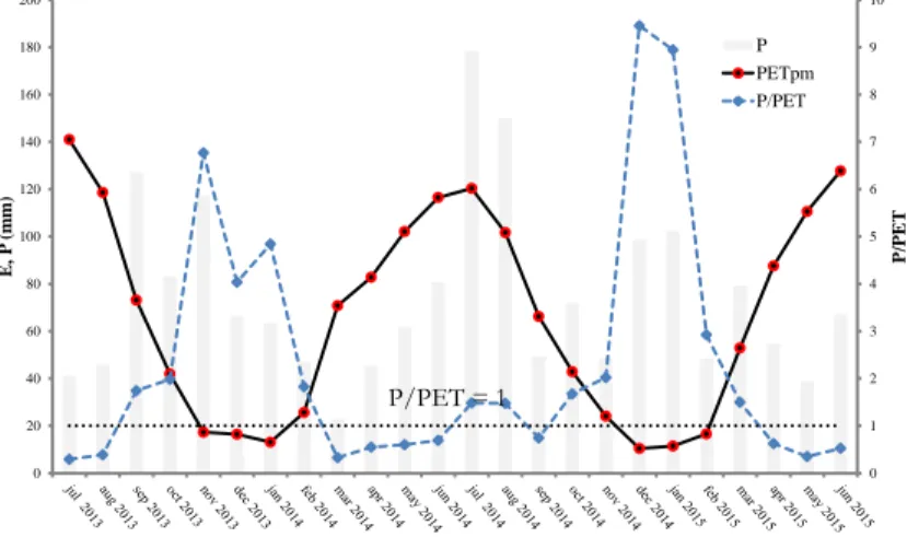
Computed on an annual time scale, for the period under evaluation, mean annual precipitation and potential evapotranspiration are respectively about 895 mm and 795 mm, which return an annual scale Budyko index of about 1.2. The energy limited scheme is thus applicable to the investigated system.

If computed at the monthly scale, the Budyko index I appears to be characterized by a seasonal pattern (Figure 3.2). From March to September I = P/PET is overall smaller than the threshold limit P/PET = 1, thus the system can be defined water-limited in this period of the year. Extra-ordinary rainfall events (not consistent with the average behaviour) occurred in July and August 2014 are the reason for I larger than 1. According to Budyko 1974 framework, actual evapotranspiration rates are controlled by precipitation amounts which are visibly significant also during this time window. From October to February I is instead larger than 1. The system switches from a water limited to an energy limited condition in this period of the year. An effective switch occurs in the period from November to February, when I values are significantly larger than 1. A comparison between actual evapotranspiration, derived by eddy covariance observations, and potential evapotranspiration, computed by the Penman Montheith formulation (Figure 3.3), illustrates how during this period (I >> 1) actual rates approach potential one and are instead lower during the remaining periods, especially during the summer season. When compared to meteorological variables available for the study site, it has been found a significant correlation between the net radiation value and the temporal switching between the water limited and energy limited conditions. At the monthly scale, in fact, actual evapotranspiration rates approach potential ones when the net radiation

(30)

assumes negative values or when net radiation is below a threshold of about 1.5 MJ/m2_d-1_. 0 1 2 3 4 5 6 7 8 9 10 0 20 40 60 80 100 120 140 160 180 200 P/P ET E, P ( m m ) P PETpm P/PET

Figure 3.2 Monthly patterns for precipitation (P), eddy covariance actual evapotranspiration (AETec), Penman-Montheith potential evapotranspiration (PETpm) and Budyko aridity index (P/PET). The dotted line P/PET = 1 represents the threshold limit between energy limited and water limited systems.

This finding, assumed valid for the particular climate environment and vegetation type considered, represent an operational result useful for further modelling the actual evapotranspiration losses, which will be constrained by potential values on the base of a threshold model that, as later detailed, can be set on widely available meteorological variables, such as the monitored net radiation.

-20 0 20 40 60 80 100 120 140 160 E, P ( m m ), Rn ( M J m −2 d −1) Rn AETec PETpm P/PET = 1

(31)

Figure 3.3 Monthly patterns for eddy covariance actual evapotranspiration (AETec), Penman-Montheith potential evapotranspiration (PETpm) and net radiation (Rn).

3.3 M

ONTHLY

AET

PREDICTION MODELS

In order to effectively model actual evapotranspiration at monthly scale, four methods have been proposed:

1) The API Antecedent precipitation index method, as described by eq.

3-13

2) The AA Advection Aridity method, as described by eq. 3-12

3) In addition to the above mentioned methods reported by the

scientific literature, two threshold combined approaches have been proposed, provided the illustrated findings related to the temporal switching from the water limited to energy limited conditions. The proposed approaches are PM/API and PM/AA models, described by eq. 3-17,3-18, combining the Penman Montheith formulation for PET assessment and the API or AA formulations for AET assessment, where the Priestley-Taylor coefficient has been set to 1.26, as suggested by Mawdsley et al. 1985. The combination between the PET and the AET formulation is proposed according to the observed temporal switch. When energy limited conditions occur, actual evapotranspiration is well described by the potential one computed by PM according to Figure 3.3 while when the system is governed by water limited conditions, actual ET rates can be accurately predicted using API and AA methods. The switch from PM to API or/and AA is detected when net radiation (NR) is below an observed threshold (NRT) as in the following:





_               _      NR_T PET_P_M R_n G_soil E_A NR if     1 , (3-17)                                      _       A soil n AA soil n API T E G R AET or G R AET NR NR if      ) ( 408 . 0 ) 1 2 ( 408 . 0 (3-18)

(32)

4) The last proposed model is the threshold approach PM/APICAL, which combines PM and API, according to the previous considerations, but where a calibration of Pristley-Taylor coefficient is further suggested in order to achieve a better fitting between observed and modelled ET values.

The relationships between AET fluxes modelled using the above described approaches and observed EC measurements have been evaluated by a quantitative fitting analysis. The comparisons help testing the ability of the models in predicting actual evapotranspiration but, what is more important, help detecting the limitations of each approach. The fitting analysis have been performed at monthly and global scales using several goodness-of-fit (GOF) indices: the root-mean-square error (RMSE), the relative error (RE), the mean absolute error (MAE), Nash-Sutcliffe Efficiency coefficient (NSE), Index od agreement (d), the correlation coefficient (r) estimated as follows:

2 1 1 2 , mod, ) (         _ 



 j n i i obsi j n ET ET RMSE (3-19) 100 (%)  obs j j ET RMSE RMSE (3-20)



   n i i obs i obs i j j ET ET ET n RE 1 , , mod, 1 (3-21)



   n i i obsi j j ET ET n MAE 1 mod, , 1 (3-22)











      n i obsi obsi n i obsi i j ET ET ET ET NSE 1 2 , , 1 2 mod, , 1 (3-23)

(33)







        n

i i obsi obsi obsi n i i obsi j ET ET ET ET ET ET d 1 2 , , , mod, 1 2 , mod, 1 (3-24) ) .( . ) .( . ) , ( var mod mod obs obs ET D S ET D S ET ET iance Co r  (3-25)

Where “j” is the index of the month, “nj“ is the length of the monthly sample, “ETmod,i” and “ETobs,i” are respectively the monthly values of modeled and observed evapotranspiration, S.D. stands for standard deviation. The monthly and global errors have been further normalized respectively by the mean monthly value and the annual cumulative value of observed AET from EC.

The results reported in Table 3.1 highlights that all of the applied models allow for a good prediction of ET and that the threshold models compared to their corresponding single models perform however better, how confirmed by the low values of RE, RMSE and MAE.

Table 3.1 Global values of the goodness-of-fit indices for the proposed models.

Method MAE (%) RMSE (%) RE (%) NSE (-) d (-) r (-)

API (1.26) 0,878 0,463 27,769 0,842 0,848 0,989

AA 0,973 0,670 36,426 0,836 0,819 0,964

PM/AA 0,869 0,279 29,707 0,855 0,826 0,935

PM/API(1.26) 0,841 0,770 25,793 0,845 0,846 0,985

PM/API(1) 0,466 0,140 20,865 0,953 0,902 0,979

At monthly scale, the results illustrated in Figure 3.4 confirm that the threshold models (eq.3-17, 3-18) have lower errors than the basic empirical models (eq. 3-12) and (eq. 3-13), with an average value of the monthly RE and RMSE respectively of 25% and 20% for PM/API(1.26) and 29% and 20% for PM/AA against 28% and 21% for API(1.26) and 36% and 23% for AA. Differences in terms of performances are evident at the seasonal scale however, with the threshold method PM/API that appear to be the best performing especially during the winter periods. In the meantime, several authors, have proposed a re-examination of the value of Priestley-Taylor coefficient in order to improve the ET prediction. Although the value proposed by Mawdsley et al. 1985 set 

(34)

on 1.26, a moderate range of variability has been reported for such coefficient. McNaughton et al. 1973 suggested to use =1.05, Davies et al. 1973 proposed a coefficient of 1.27 while Morton 1983 of 1.32 similar to 1.3177 proposed by Hobbins et al. 2001. De Bruin et al. 1979 further argued about a variation of  between 1.15 and 1.42. Given the uncertainty in the value to be assigned to the Priestly Taylor coefficient and in order to improve the simulation approach, a calibration of the value of the Priestley Taylor coefficient is also here proposed.

(35)

The calibration is performed, at the monthly scale, with reference to the API method formulation eq. 3-13 from which the  coefficient is computed according to:

soil n j obs CAL j G R AET         , 1 ,    (3-26)

where the AET losses is assumed to correspond to the observed eddy correlation values, where “j” is the index of the month.

The calibration particularly concerns only the periods when the system can be defined water-limited excluding those ones where energy limited conditions prevail, as during these periods the evapotranspiration is well described by the potential PET. The monthly calibration (Figure 3.5) show a value of  approximately equal to 1 for all the periods when water limited conditions occur.

Figure 3.5 Calibrated monthly values of the Priestly Taylor coefficient .

The accuracy of the ET values provided by the calibrated API models with aCAL=1 has been verified and compared to those ones resulting from the non-calibrated approach using the above said goodness of fit indices (Figure 3.6). The monthly indices computed for the PM/APICAL confirm that the process of calibration involving the adjusted coefficient

 allows to a further improvement of the PM/API model with an average monthly RMSE of 11% compared to 20% of the threshold

(36)

model PM/API and a minimum value of 0.06 % against 1.53%. At the global scale (Table 3.1), the indices for PM/APICAL model appear overall the best performing in the end, the calibration of the Priestly-Taylor coefficient appears to be a critical issue in the improvement of model performances.

(37)

4 DAILY SCALE WATER BALANCE

MODEL

The proposed threshold methodology for an accurate simulation of the actual evapotranspiration loss simply based on meteorological data can be used in retention models for the prediction of green roof retention performances. Until now, questions remain to be answered regarding the relationship between the complexity level of a GR retention model and its performances. Three conceptual models, of increasing complexity in descriptive details, are calibrated and compared to experimental data of runoff recorded over three years from an experimental site located at Bernkastel-Kues, Germany. The case study has enable to determine if higher complexity level leads to better model performance, and therefore to a better prediction of observed hydrological processes. The proposed approaches consist of daily scale hydrological models, based on water balance equations, where the main processes and variables accounted for are the precipitation input, the evapotranspiration losses and the maximum water storage capacity. Model detail increase is achieved moving from a basic approach using potential evapotranspiration and constant storage threshold to an intermediate complexity approach using actual evapotranspiration and a constant storage threshold to an advanced approach using actual evapotranspiration and a variable storage threshold. Potential evapotranspiration has been estimated with the use of the Penman–Monteith equation while actual evapotranspiration with the proposed threshold combined approach. The maximum water holding in the basic and intermediate approach is the only model parameter to be calibrated for hydrological simulation, it depends on substrate layer material properties and represents a constant physical property. In the advanced approach the storage threshold represents a process and it is a variable evolving over time. The model estimates of runoff have been compared with observed runoff data for the entire duration of the study period using two fit indices namely the average of absolute percentage errors (AAPE) and root-mean-square errors (RMSE). The main findings confirm on one side the role played by evapotranspiration modeling and, on the other side, the good accuracy

(38)

achieved, in a minimal calibration requirement approach, through the modeling of basic and elemental processes.

4.1 T

HE STUDY SITE AND DATA

The green roof in analysis is an extensive green roof with an area of 22 m2_{and a slope of about 5°, it is located in Bernkastel-Kues (49° 55’ 11”} N, 7° 4’ 33” E, 145 m above sea level), Rhineland-Palatinate, western part of Germany (Figure 4.1).

Figure 4.1 Green roof location and composition.

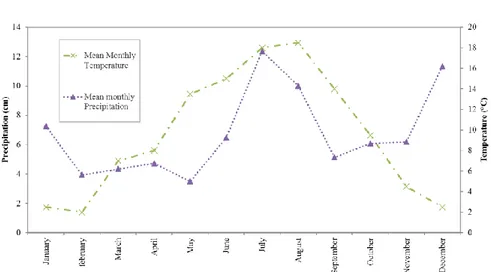
It is made up of three layers: the vegetation layer (spontaneous vegetation), the growing medium (mineral substrate) consisting of a mixture of lava, pumice and humus and a water storage/protective layer (retention Hydrotex membrane). The climate regime is typically oceanic. Average precipitation is about 700–800 mm/year and it is approximately uniformly distributed during the year. Temperature exhibits instead a typical seasonal pattern, with highest monthly mean values during the summer season of about 18 °C and annual average temperature of 9,4° (Figure 4.2).

(39)

Figure 4.2 Patterns of mean monthly rain and temperature for the study site.

Meteorological data are precipitation recorded at the experimental site and wind speed, air temperature, relative humidity, global radiation collected at the nearest available meteorological station, Bernkastel (AgrarMeteorologie, Rheinland-Pfalz, 2017). Runoff measurements have been recorded, with a daily time step, from March 2004 to May 2007, but some missing data appear during the monitoring period, preventing the total period of observation to be used for modeling purposes. Generally, no significant runoff has occurred, due to freezing of the water, between late December and late March. For this reason, the winter period has not been considered in the simulation approach.

4.2 T

HE CONCEPTUAL MODELS

The aim of the reported research is an analysis of the impact of the complexity in the description of variables and processes of a green roof hydrological model on the relative parameterization and accuracy, with a focus on the retention capacity of the green infrastructure. To this purpose a daily scale conceptual hydrological model is applied, based on water balance equations whose main input variables are the precipitation, the evapotranspiration loss and the maximum water storage capacity, here called storage threshold (Mobilia et al. 2017). The model is used

(40)

with three different settings (mod A, mod B and mod C), characterized by an increasing complexity in the description of the involved variables and processes (Table 4.1).

Table 4.1 Models settings for different model complexity level. Mod A represents the basic approach. Mod B represents the intermediate approach. Mod C represents the advanced approach.

Model ET Wmax

Mod A PET Constant

Mod B AET Constant

Mod C AET Variable

The three settings correspond to: a basic approach based on the use of potential evapotranspiration and a constant storage threshold (mod A); an intermediate approach where actual evapotranspiration and a constant storage threshold are accounted (mod B); an advanced approach where actual evapotranspiration and a variable maximum water holding depth are used (mod C). The three conceptual retention models, of different complexity, are calibrated using the values of runoff measured from the studied infrastructure.

4.2.1 The governing equations

The water balance equations used to simulate the runoff production “R”, common to all of the three model settings, are:

                       max 1 max max 1 max 1 0 W ET P V W V R W ET P V V R W ET P V V t t t t t t t t t t t t t t (4-1)

where “t” is the daily time index, “V” the green roof water depth, “P” the observed precipitation, “ET” the modelled evapotranspiration loss, “Wmax” the maximum water holding depth or storage threshold.

In the basic approach, ET loss is assumed to be set on the potential evapotranspiration (PET) and a constant storage threshold is also considered. The governing equations become:

                       max 1 max max 1 max 1 0 W PET P V W V R W PET P V V R W PET P V V t t t t t t t t t t t t t t (4-2)

(41)

where the term “ETt” is replaced by “PETt”. As PET is rapidly computed from meteorological observation, Wmax represents the only model parameter to be calibrated.

Potential evapotranspiration represents obviously an ideal process, but for a better model performance, the actual evapotranspiration process should be modeled (Mobilia et al. 2016b). Actual evapotranspiration AET modeling generally requires soil moisture, soil and vegetation properties data, but in order to keep to a minimum the number of needed information, an approach simply based on meteorological variables and on the concept of non-potential Priestley-Taylor model (Mawdsley et al. 1985), is in the following used. In the intermediate complexity approach, ET loss is then assumed to be set on the non-potential Priestley-Taylor evapotranspiration (AET) and a constant storage threshold is accounted for. The governing equations are represented by eq. 4-3 where the term “ETt” is replaced by “AETt”:

                       max 1 max max 1 max 1 0 W AET P V W V R W AET P V V R W AET P V V t t t t t t t t t t t t t t (4-3)

As in the case of the basic model, also in this case Wmax represents the only parameter to be calibrated for hydrological simulation. Considered as the amount of water stored between the permanent wilting point and the field capacity, the maximum water holding capacity Wmax depends on substrate layer material properties and represents a constant physical threshold. The constant physical limit could be however called into discussion, if it is considered that due soil heterogeneity runoff can occur even before the actual capacity is reached and that vegetation provides some additional moisture storage capacity to be accounted for (Poë et al. 2015). Wmax is more likely to represents a process rather than a physical property and, as exhaustively discussed in Mobilia et al. (2017), a strong correlation is found between the maximum water holding depth on day “t” and the water depth on day “t − 1” as follows:

1 max,t Vt

W (4-4) The correlation results from the eq. 4-3, where the GR runoff production is computed at the daily scale as:

(42)

max 1 max mod , V W V P AET W Rt  t   t  t  t  (4-5) If Eq. 4-5 is reversed, a calculation for Wmax could be obtained:

mod . 1 mod , max,t Vt Rt Vt Pt AETt Rt W    _    (4-6) Assuming further that for each day t, the modeled runoff (Rmod) is equal to the observed one (Robs), a calibrated daily time series for Wmax,t can be obtained: obs t t t t t V P AET R Wmax,  1   . (4-7) Plots for Vt - 1 and Wmax,t are provided in Figure 4.3, as a ratio of the green roof depth.

Figure 4.3 Water depth (V) and water holding capacity (W) daily scale patterns as a ratio to soil depth. Actual evapotranspiration losses are computed by the API Method. Overlapped, in the upper right corner, the scatter plot for the two considered variables and the relevant Person correlation coefficient.

Illustration refers to AET computed by the threshold method

PM/API(1.26). Considering the above discussed soil physical properties and

also probably to balance the a-priori calculation for AET losses, Wmax becomes a variable for the GR hydrological model itself. Its temporal pattern is nearly coincidental with the water depth pattern. Retention