The Effects of Air Pollution on COVID‑19 Related Mortality
in Northern Italy
Eric S. Coker1 · Laura Cavalli2 · Enrico Fabrizi3 · Gianni Guastella2,4 ·
Enrico Lippo2 · Maria Laura Parisi5 · Nicola Pontarollo5 · Massimiliano Rizzati2 · Alessandro Varacca6 · Sergio Vergalli2,5
Accepted: 13 July 2020 © The Author(s) 2020
Abstract
Long-term exposure to ambient air pollutant concentrations is known to cause chronic lung inflammation, a condition that may promote increased severity of COVID-19 syndrome caused by the novel coronavirus (SARS-CoV-2). In this paper, we empirically investigate the ecologic association between long-term concentrations of area-level fine particulate matter (PM2.5) and excess deaths in the first quarter of 2020 in municipalities of Northern Italy. The study accounts for potentially spatial confounding factors related to urbanization that may have influenced the spreading of SARS-CoV-2 and related COVID-19 mortality. Our epidemiological analysis uses geographical information (e.g., municipalities) and neg-ative binomial regression to assess whether both ambient PM2.5 concentration and excess mortality have a similar spatial distribution. Our analysis suggests a positive association of ambient PM2.5 concentration on excess mortality in Northern Italy related to the COVID-19 epidemic. Our estimates suggest that a one-unit increase in PM2.5 concentration (µg/m3) is associated with a 9% (95% confidence interval: 6–12%) increase in COVID-19 related mortality.
Keywords COVID-19 · Mortality · Pollution · Italy · Municipalities
JEL Classification Q53 · I18 · J11
* Gianni Guastella
1 College of Public Health and Health Professions, University of Florida, Gainesville, FL, USA 2 Fondazione Eni Enrico Mattei, Milan, Italy
3 Department of Economics and Social Sciences, Università Cattolica del Sacro Cuore, Piacenza,
Italy
4 Department of Mathematics and Physics, Università Cattolica del Sacro Cuore, Brescia, Italy 5 Department of Economics and Management, Università degli Studi di Brescia, Brescia, Italy 6 Department of Agricultural Economics, Università Cattolica del Sacro Cuore, Piacenza, Italy
1 Introduction
With more than twelve million confirmed COVID-19 cases and more than 550 thousand related deaths globally as of the beginning of July 2020,1 the novel coronavirus pandemic has unquestionably caused dramatic health and economic impacts. Despite the public health benefits of the consequent COVID-19 mitigation measures adopted by the central and the regional governments in Italy, one of the most heavily impacted countries, there are adverse socioeconomic effects of the lockdown on top of what are already dramatic public health impacts. Official morbidity statistics, although complicated by the public health interventions and the emergency status, reveal a strong spatial clustering phenom-enon across administrative regions in Italy and provinces and municipalities within each region. Such a geographical concentration of both COVID-19 morbidity and mortality is most likely the result of the interaction of multiple factors, among which include the clus-tering of initially infected individuals, different choices made about testing and contact tracing in order to identify community transmission, underlying population demographic and prevalence of health status, and the timely adoption of lockdown measures to control the COVID-19 epidemic (Ciminelli and Garcia-mandicó 2020). Beyond such proximal fac-tors, however, additional contextual factors may have played an important role in the health impacts of COVID-19 in Italy.
The Northern Italian regions most affected by the spreading of coronavirus (Lombar-dia, Veneto, Piemonte, Emilia Romagna) are also the most densely populated and heavily industrialized and thereby the most heavily polluted regions of Italy. These four regions together host 39% of the national population,2 and approximately one-half of the Ital-ian GDP is produced there. Such a spatial concentration of economic activities involves the industrial manufacturing sectors to the largest extent, and the consequent high level of emissions is at least in part responsible for poor air quality in the region.3 In Brescia, among the most affected cities in Lombardy, the concentration of particulate matter (PM) and ozone exceeded the allowable threshold in 150 days in 2018, making it the most pol-luted city in Italy. Lodi and Monza follow, with 149 and 140 exceedance days, respectively. Milan and Bergamo are sixth and ninth, respectively, with 135 and 127 days.4 Lombardy is also among the most polluted regions in all of Europe (European Environmental Agency
2019). The relatively higher air pollutant concentrations in the Po Valley region of Italy contrasts sharply with neighbouring alpine regions and stems from the combination of two main factors (Carugno et al. 2016; Larsen et al. 2012; Pozzer et al. 2019). The first is the high concentration of urban areas with their congested roads and industrial belts. Source apportionment research from the Lombardy region (Pirovano et al. 2015) indicates that the major sources of PM2.5 include residential heating (e.g., fuel), transport, agriculture, background (including natural-source sand long-range transport), and other (including sta-tionary industrial sources). The second is the location in the orographic “bowl” of the Po
1 Data from Johns Hopkins coronavirus resource center, updated July 10. 2 At January 1st 2019, source: Italian Bureau of Statistics—ISTAT.
3 Different components of gas emissions (e.g. nitrogen dioxide, carbon monoxide), derive from many
activities like traffic congestion, house heating, agricultural and husbandry practices, as well as industrial combustion. Concentrations are characterized by seasonality, with high levels in Winter, and weather condi-tions, however the 2020 lockdown measures reduced substantially those derived from traffic but not those derived from agricultural activities (ARPA Lombardia 2020).
4 Data from the annual report on air quality in Italian cities by Legambiente, available at https ://www.
Valley, an extension of flat river lands enclosed between the Alps and Apennines moun-tains, which causes the stagnation of pollutants due to low ventilation (Giulianelli et al.
2014).
These factors help to characterize the Po Valley’s peculiarity with respect to different European areas with comparable urban and industrial density levels (Eeftens et al. 2012). Moreover, in addition to the urbanized and industrial areas, the remainder of the valley presents an intensive agricultural activity. Local studies on emission sources highlight a varying composition of the final concentration values depending on the position of moni-toring stations and with different sources acting as local or diffused ones (for instance hav-ing high emissions from traffic close to cities, while havhav-ing background biomass burnhav-ing diffused in the whole region) (Bigi and Ghermandi 2016; Larsen et al. 2012). Indeed, given the EU Ambient Air Quality Directives that sets the Air quality standards for the protection of health at 25 μg/m3 for the averaging period of a calendar year, the Po valley shows val-ues consistently near or above the threshold. These valval-ues often range in the 25–30 μg/m3 interval with peaks of > 30 μg/m3, which in Europe are only matched in Southern Poland and other smaller Eastern European clusters (EEA 2019).
Compared to its overall representation in the population, Lombardy is disproportion-ately impacted by 19 related mortality, with approximdisproportion-ately 53% of Italy’s COVID-19 deaths as of April 15, 2020 (Odone et al. 2020). Lombardy is also the most impacted Italian region as far as the total number of deaths in excess in the first quarter of 2020 com-pared to the same period of the previous years. Comparing the official COVID-19 death data with registry deaths, it emerges that the latter is almost 70% larger than the former in Lombardy, 27% larger in Emilia-Romagna and 18% and 16% in Veneto and Piemonte, respectively. It is, therefore, imperative to consider the role that PM may have played in such disproportionate COVID-19 deaths in Northern Italy.
There are a number of plausible pathways by which airborne PM may impact COVID-19 related morbidity and mortality. Existing data already finds a strong positive correlation between viral respiratory infection incidence and ambient PM concentrations (Ciencewicki and Jaspers 2007; Sedlmaier et al. 2009). One plausible pathway for this phenomenon is the fate and transport of the virus itself within the environment. A recent position paper by the Italian Society of Environmental Medicine argues that PM may act as both a carrier and substrate of the virus and thus influence the virus’ fate and transport in the environ-ment and reaching susceptible receptors (Setti et al. 2020). Another pathway is the increase in susceptibility to COVID-19 mortality caused by long term exposure to PM. Fine PM is already known to affect cardiovascular and respiratory morbidity and mortality (Cakmak et al. 2018; Jeong et al. 2017; McGuinn et al. 2017; Yin et al. 2017). Moreover, among 1596 Italian COVID-19 patients who died in the hospitals, and for whom it was possible to analyze clinic charts, data showed substantial comorbidities including ischemic heart dis-ease (27.9%); atrial fibrillation (22.4%); heart failure (15.6%); stroke (10.9%); hypertension (70.6%), and chronic obstructive pulmonary disease (17.9%) (Istituto Superiore di Sanità
2020). Biologically, long-term PM exposure may be responsible for a chronic inflamma-tion status that causes the hyper-activainflamma-tion of the immune system and the life-threatening respiratory disorders caused by COVID-19 (Shi et al. 2020).
Some preliminary evidence is now emerging about COVID-19 that shows a positive relationship between air pollution and morbidity and mortality. Beyond qualitatively describing the European Air Quality Index for Northern Italy to argue the causal role of air pollution and the relatively high COVID-19 mortality observed in that region, Conti-cini et al. (2020) review the most recent existing toxicological and epidemiological litera-ture. Based on existing evidence from other empirical studies, they clarify the relationship
between air pollution, prolonged inflammation and immune system hyper-activation and immune suppression, and the link between the latter and acute respiratory distress syn-drome, and respiratory mortality. Their paper is important in that it suggests a clinical and biologically plausible explanation to our analysis, but does not provide statistical evidence in support of the hypothesis. A separate empirical analysis by Becchetti et al. (2020) finds preliminary evidence that confirms such a positive effect of air pollution on mortality in Italy based on the analysis of death data at the province level. Similarly, Wu et al. (2020) show a positive association between long term PM exposure and COVID-19 related deaths in US counties. Ogen (2020) recently analysed data from 66 administrative regions in France, Spain, Italy, and Germany, and found that the highest COVID-19 deaths in these regions were associated with five regions of Northern Italy that also corresponded with the highest levels of atmospheric nitrogen dioxide (NO2). Cole et al. (2020) estimate the same relationship using Netherlands municipality data and find PM2.5 positively associated with COVID-19 cases, hospitalization, and deaths.
In this paper, we follow this emerging stream of the empirical literature and test the hypothesis that a higher average long-term exposure to PM2.5 is positively associated with the current extraordinarily high death toll in Northern Italy. We decided to focus on PM2.5 because, given the complexity of air pollution, it is quite common in air pollution epide-miology studies to focus the analysis on a single pollutant (Wu et al. 2020), although mul-tipollutant analyses are certainly warranted. We selected PM2.5 for a variety of important reasons, including policy implications and evidence in the literature in terms of chronic health effects. Regarding its policy implications, we selected PM2.5 as opposed to PM10 because the former is more correlated with human activities than the latter, and it cor-relates with stronger health effects than PM10 does. With respect to respiratory mortality effects from the existing air pollution literature, the most robust evidence points to PM2.5 as opposed to other gaseous air pollutants (Bowe et al. 2019).
Mortality data are collected at the municipality level for the period January-April 2020. Given that mortality data are not disaggregated by mortality cause, death counts are meas-ured as the difference from the last five-years mean to reflect the abnormal number of deaths caused by the spreading of the pandemic. Since PM2.5 can be associated to generic mortality even in the absence of the pandemic outbreak (Dominici et al. 2003; Katsouyanni et al. 2001; Samet et al. 2000), we also estimate the impact of PM2.5 on the excess mortal-ity in the sample using 2019 data, a time in which the coronavirus epidemic had presum-ably not yet begun. Data on PM2.5 concentration at the municipality level refer to the years prior 2020 to account for long-term population exposure. We assign municipality PM2.5 concentration by a set of different methods of spatial interpolation (kriging) of monitoring station data related to the years 2015–2019.
We estimate a negative binomial model of excessive deaths on historical PM2.5 concen-trations and a series of control variables that may plausibly affect both PM2.5 concentra-tion and mortality, including populaconcentra-tion density; the spatial concentraconcentra-tion of the industrial manufacturing sites; climatic conditions observed during the first quarter of 2020; and the demographic composition of the municipal population among others. In addition, we con-sider spatial heterogeneity in the distribution of the number of deaths related to regional and local unobservable factors. We account for region-specific effects because regions, in Italy, are the administrative units in charge of managing the health systems and the meas-ures taken to trace and contrast the spreading of the pandemic varied greatly among even contiguous regions. We also account for local effects common to functionally linked clus-ters of municipalities (the Local Labour Systems—LLS). We deem this part of the identi-fication strategy crucial because the relationship between PM2.5 and COVID-19 mortality
may be confounded by several other factors, some of which were not observable or measur-able, but are nevertheless intrinsically related to the geographical location of the observed units.
The remainder of the paper is organized as follows. The next section introduces the empirical strategy and describes the dataset. The results are presented and discussed in sec-tion three, considering the total number of (excess) deaths. Secsec-tion four draws the conclu-sions and highlights the limitation of the study and the indications for future research.
2 Empirical Strategy and Data
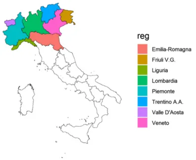
Our analysis is restricted to the study area of Northern Italy (Fig. 1), which encompasses the sub-regions of Valle D’Aosta, Piemonte, Liguria, Lombardia, Emilia-Romagna, Veneto, Friuli-Venezia Giulia and Trentino-Alto Adige/Südtirol. Official territorial data on COVID-19 mortality in Italy are available at the rather aggregate regional or provincial level, cor-responding to the levels 2 and 3, respectively of the European nomenclature units for ter-ritorial statistics (NUTS).5 In addition, these official data refer to the deaths of patients tested positive for severe acute respiratory syndrome coronavirus 2 (SARS-CoV2) only and do not include (potential) patients without COVID-19 diagnosis because they were not tested and died at home or elsewhere. Hence, the officially reported deaths are likely underestimated. Because testing policies vary among regions in Italy, the induced measure-ment error is also non-randomly distributed among the provinces. Ciminelli and Garcia-mandicó (2020) compare the official COVID-19 fatality rates with historical death data and
Fig. 1 Italian regions included in the study
report that deaths were higher than official fatalities throughout the period of COVID-19 epidemic.
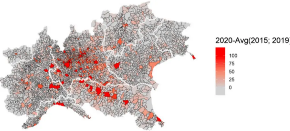
Working under the assumption that COVID-19 deaths are underestimated in Italy, the choice is made in this paper to use the total deaths from the official registries, accordingly, and to scale the analysis at the municipality level, the smallest administrative units, to have a more granular representation of the spatial dimension of the phenomenon. Since we are interested in excess deaths, we take the difference between the number of deaths in the period January 1—April 30, 2020, and the average number of deaths in the same period of the previous 5 years (ExDeaths) and use this metric as the dependent variable in our sta-tistical model. Figure 2 displays the geographical distribution of the above-described data among the 4041 municipalities for which data is available.
The variable is assumed to follow a Negative Binomial distribution, a generalization of the Poisson distribution that avoids the restrictive mean–variance equality of the latter, and is modelled as follows:
where 𝜃 is the overdispersion parameter to be estimated and 𝜇i is the municipality-specific expectation conditional on the value of the covariates. Among the covariates, PM is the concentration of fine particulate matter in municipality i and 𝛽 is the associated parameter, which we expect positive and statistically different from zero; X is a vector of control vari-ables that adjusts for the potential confounding effects and includes the (log of) total popu-lation as the offset while 𝜀 is a normally-distributed error term.
Our main source of PM2.5 data is the European Environmental Agency’s (EEA) air monitoring database, which is provided to EEA by the Institute for Environmental Pro-tection and Research (ISPRA). ISPRA conducts ground-level air measurements of PM2.5 air concentrations (µg/m3) collected at 268 monitoring sites throughout Italy. Specifically, we use the EEA’s E1a and E2a datasets, which are primary validated assessment data and primary up-to-date assessment data reported by the European Member States, respectively. Although the measurements come both in hourly and daily averaging formats, we work (1) ExDeathsi∼NB(𝜇i, 𝜃
)
log(𝜇i) = 𝛼 + 𝛽PMi+ 𝛿�Xi+ 𝜀i
Fig. 2 Spatial distribution of cumulative excess deaths in sample municipalities, Northern Italy, January 1—April 30, 2020
with daily values and use them to obtain yearly aggregates for the years 2015, 2016, 2017, 2018, and 2019. However, because model (1) does not include a time component, we fur-ther compute a six-year averaging time to obtain a metric of long-term (chronic) PM2.5 concentration levels throughout different spatial units of Northern Italy. The number of 6 years for the reference period is sufficiently long to account for long-term exposure while being not too long to be affected by the mobility of people among municipalities, and it is in line with existing literature assessing long-term effects of PM exposure (Yorifuji et al.
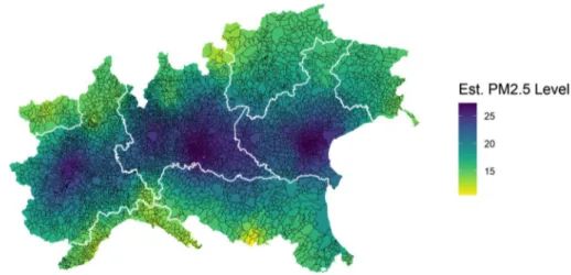
2019). Since the air monitoring stations provide only partial spatial coverage for munici-pality-level PM2.5 concentration data, we impute missing observations using a spatial inter-polation model. Specifically, we fill in the gaps using a mean stationary Ordinary Kriging (see Bivand et al. 2013, p 209) defined through an exponential covariance function with nugget, partial sill and range parameters estimated through (restricted) maximum likeli-hood methods. Figure 2 displays the resulting PM2.5 concentration data.6
Comparing Figs. 2 and 3, it is possible to visually appreciate a spatial coincidence between higher levels of excess mortality and higher levels of PM2.5, in particular in the Lombardia region which notably is the region with both the highest particulate concentra-tion and the highest number of excess mortality.
The hypothesis that PM2.5 concentration affected COVID deaths, that is ̂𝛽 > 0 , is tested among several possible specifications. In model (2) we include regional effects (𝜆j
) . These effects are expected to capture the aspects related to the management of the outbreak, which may have systematically influenced COVID-19 mortality and that are common to all the municipalities in the same region. Italy has a national health system that ensures equal access to healthcare to all citizens. The system is managed by regions at the local level, and, in the specific case of this pandemic, regions were responsible for defining the testing and contact-tracing protocols and implementing the necessary measures to contain the out-break, among which the measure to protect healthcare workers. In model (3), we include
Fig. 3 Spatial distribution of PM2.5 concentration levels in the sample municipalities, simple kriging of monitoring stations, average across years 2015–2019
6 We also replicate the analysis using other trend-stationary models (i.e. universal kriging) and different
LLS-specific effects (ek )
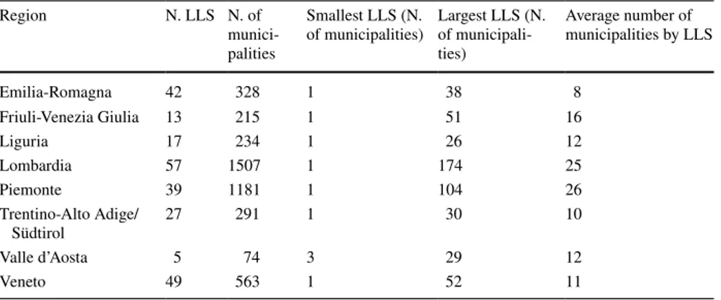
. LLS are spatial clusters of contiguous municipalities related by commuting flows that share a common specialization in a specific sector of manufactur-ing production and correspond to the conceptualization of Marshallian districts (Becat-tini 2002). The number of LLS clusters per-region and the total number of municipalities belonging to clusters are reported in Table 1, along with the minimum, maximum, and average cluster size.
The use of LLS captures the interlinkages within neighbouring municipalities that may have favoured the geographical spreading of coronavirus around specific hotspots. Mortal-ity data are then expected to vary among municipalities in different LLS, but differences are expected to be non-systematic in this case. In model (4) we include both the regional fixed effects and the LLS random effects.
Control variables to be included in the model were chosen to avoid any potential spatial confounding effect and considering as well the emerging literature on the impact of PM on COVID-19 related deaths (Cole et al. 2020; Wu et al. 2020). The population density and per-capita income account for urbanisation level. The most densely populated and wealthy municipalities are among the most polluted due to the spatial concentration of manufac-turing and service activities but are also the places where the contagion could have been easier, with a potential impact on mortality. In addition to the density of population, the (2) ExDeathsi∼NB(𝜇ij, 𝜃 ) log(𝜇ij) = 𝛼 + 𝛽PMij+ 𝛿�X ij+ 𝜆j+ 𝜀ij (3) ExDeathsi∼NB(𝜇i, 𝜃) log(𝜇ik) = 𝛼 + 𝛽PMik+ 𝛿�Xik+uik uik= 𝜀ik+ek (4) ExDeathsi∼NB(𝜇ijk, 𝜃)
log(𝜇ijk) = 𝛼 + 𝛽PMijk+ 𝛿�Xijk+ 𝜆j+uijk uijk= 𝜀ijk+ek
Table 1 Number of LLS spatial clusters in each region
Region N. LLS N. of
munici-palities
Smallest LLS (N.
of municipalities) Largest LLS (N. of municipali-ties) Average number of municipalities by LLS Emilia-Romagna 42 328 1 38 8 Friuli-Venezia Giulia 13 215 1 51 16 Liguria 17 234 1 26 12 Lombardia 57 1507 1 174 25 Piemonte 39 1181 1 104 26 Trentino-Alto Adige/ Südtirol 27 291 1 30 10 Valle d’Aosta 5 74 3 29 12 Veneto 49 563 1 52 11
shares of municipality area occupied by industrial sites and the average size of manufac-turing firms are included in the regression because they are related to pollutant concentra-tion and possibly to mortality. Naconcentra-tional measures to stop the spreading of the viral infec-tion (lockdown) involved the service sector to the largest extent while many manufacturing activities, being considered necessary, were left open and, in the absence of social distance and individual protection measures, the geographical concentration of these activities in a municipality with their complex logistics and transport interconnections, and the size of plants, may have influenced mortality. Average temperature, for which an association with COVID-19 deaths has also been found (Ma et al. 2020), is also included in the regres-sion.7 Moreover, COVID-19 incidence has proven to be higher among men than women and people aged 65 or more. Hence these two variables are considered in the model, even though these aspects are not necessarily connected with the average PM2.5 exposure in a municipality. Underlying socioeconomic conditions can also play a role in COVID-19 related mortality (Goutte et al. 2020). Brandt et al. (2020) and Mukherji (n.d.) have shown that, in the US, COVID-19 is more threatening for ethnic minorities, and we believe that the share of migrants, identified as non-EU citizens, can control for this aspect influencing the observed excess mortality. On the other hand, Mukherji (2020) and Goutte et al. (2020) also find that places with a higher share of the population with a low level of education have higher deaths. In our paper, given the lack of updated data on education at the munici-pal level, we proxy it with the percentage of university students on the total population. The distance from the closest airport is a proxy for the functional and relational linkage between a municipality and a place of highly frequent national and international connec-tions and potential sources of coronavirus spreading. Finally, we consider the number of hospital beds as a proxy for the supply of health services to account for the fact that many people died at home without being diagnosed for coronavirus due to the shortage of beds in public structures. The full details of the variables in the model, including sources and sum-mary statistics, are presented in Table 2.
Having accounted for the confounding effect due to the omission of relevant informa-tion from the empirical specificainforma-tion, we exclude any other potential source of endogeneity considered in similar papers. In particular, we exclude endogeneity due to measurement error in the outcome variable and the main independent variable. Concerning the outcome variable, the relationship between deaths and cases with fine PM could be spurious because more cases could be registered, and more individuals tested in highly polluted areas as people there are more likely to show COVID-19 symptoms due to the chronic inflamma-tion induced by PM. The high toll of deaths of people diagnosed with COVID-19 would be a natural consequence of that. In contrast, the number of deaths in excess, used in this paper, is not affected by testing problems since it considers all the potential COVID-19 deaths. Concerning the PM variable, measurement errors are likely to occur when using satellite data or modelled data. We preferred to use PM2.5 levels observed from monitoring stations to avoid such a measurement error. Some caution is needed in the spatial inter-polation because the method chosen to fill the missing data may underestimate the value in locations farther from the monitoring stations. With this concern in mind, we test the robustness of our results using PM2.5 data obtained from different interpolation approaches.
7 We omit average humidity because the variable shows a too strong linear correlation (ρ= 0.98) with
temperature in our sample observations, and its inclusion would cause severe imperfect collinearity in the model.
Table 2 Descr ip tion of model v ar
iables and summar
y sam ple s tatis tics Var iable Descr ip tion Mean Median SD ExDeat hs Number of deat hs in t he per iod Januar y 1—Apr il 30 2020—absolute differ ence com par ed t o t he a ver ag e of the pas t fiv e y ears, sour ce: IS TA T 9.32 2 37.13 PM 2.5 Fine (2.5 µg/m 3) par
ticulate matter concentr
ation obt ained b y spatial inter polation of monit or ing s tations, av er ag e acr oss t he y ears 2015–2019, sour ce: Eur opean En vir onment al A gency 19.67 20.85 4.15 Pop. density
Population density com
puted as t
ot
al population in number of inhabit
ants on Januar y 1 2020 o ver t he t ot al ar tificial ar ea in Km 2, sour ces: IS TA T and Eur opean En vir onment al A gency—Cor ine land Co ver dat a 34.44 14.69 58.19 PC income Av er ag e per -capit a income, sour ce: Minis try of F inance, 2019 15,658.46 15,564.52 2497.44 % Ind. Land Shar e of indus trial ar ea on t ot al municipality sur face measur es t hr
ough satellite obser
vation, sour ce: Eur o-pean En vir onment al A gency—Cor ine land Co ver dat a 2.62 0.02 5.17 % Small Ent Shar e of enter pr ises wit h less t han 10 em plo yees, sour ce: R egis tro s tatis tico delle U
nità Locali (ASIA—UL)
94.26 94.44 3.80 Tem per atur e Av er ag
e mean skin tem
per atur e dur ing t he deat h obser vation per iod, sour ce: Coper nicus ERA5 0.25° × 0.25° gr id r esolution dat ase t. 3.75 5.34 4.01 Female/Male Ratio be tw een f
emale and male population, sour
ce: IS TA T 1.01 1.02 0.06 % Ov er 65 Shar e of population older t han 65, sour ce: IS TA T 23.36 22.72 4.93 % non-EU Shar e of non-EU r esidents, sour ce IS TA T 1.88 1.51 1.55 % U niv . S tud. Definition, sour ce: shar e of U niv ersity s tudents o ver t ot al population, sour ce: Minis try of U niv ersity and Resear ch 82.28 19.49 289.57 Dis t. Air por t Dis tance in me ters t o t he closes t Air por t, sour
ce: our com
put
ation based on Eur
opean En vir onment al Ag ency—Cor ine land Co ver dat a 23,255 21,437.22 12,823.72 PC Hospit al Beds Number per -capit a hospit al beds in t he municipality , sour ce: Healt h Minis try 0.001 0.00 0.012 Population To
tal population, sour
ce: IS TA T 6710.32 2549 38,814.47
3 Results
As indicated in Table 2, the overall average of PM2.5 for the study area between 2015 and 2019 is roughly 20 µg/m3, as most municipalities in Norther Italian regions belong to industrial and agricultural intensive locations. The average mortality between 2015 and 2019 for the period of interest (January 1—April 30) was 25 deaths, while it grew to 34 in 2020. That results in an average excess death of 9, with standard deviation four times as larger (see Table 2).
Estimation results from the negative binomial models are summarised in Table 3 for the four different specifications of the model (1—no geographical effects; 2—regional fixed effects; 3—LLS random effects; 4—regional fixed effects and LLS random effects). In the lower part of the table, the estimated overdispersion parameter, the Akaike Information Criterion (AIC), and the Moran’s test for the null hypothesis of absence of spatial autocor-relation8 in the residuals (Moran 1950) are reported.
The four specifications provide consistent results in terms of the direction and signifi-cance of PM2.5 coefficients. The overall effect of PM2.5 on COVID-19-related excess mor-tality is positive and statistically significant in all models. The estimated incidence rate ratios, reported in Table 4 with their confidence interval, for Model 1, 2, 3 and 4 are 13.7%, 8.9%, 9.3%, and 9.3%, respectively.
In model 2, the regional fixed effects coefficients are statistically significant. They indi-cate that other things being equal, the number of deaths in municipalities in Lombardy and Emilia Romagna has been systematically higher compared to base category9 and in munic-ipalities in Veneto it has been systematically lower. The significance of the coefficient for Emilia Romagna, however, drops after including the random effects in the model. Since the first three models are nested into model 4 it is also possible to compare the models in terms of AIC. Model 4 performs substantially better than the other three. In general, the inclu-sion of RE in models 3 and 4 leads to a decrease in the value of the AIC. In models 1 and 2 the residuals appear spatially autocorrelated, as the null hypothesis of no spatial autocor-relation is rejected in both cases (p < 0.001). The introduction of the LLS random effects appears to solve the issue of autocorrelation.
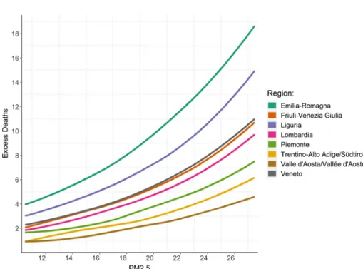
Based on the estimates of model 4, we compute the expected value of excess deaths conditional on covariates (taken at the average level) in the average city for varying levels of PM2.5 and show how the expected number of deaths by region varies at different concen-tration levels in Fig. 4. Notably, Emilia–Romagna and Liguria are the regions in which a a reduction of average fine PM from the highest level to the lowest would have benefited the most.
3.1 Robustness checks
For robustness check of the PM2.5 metric used in our study, we explored the influence that other alternate PM2.5 metrics may have on the direction and magnitude of the observed associations. Figure 5 depicts the point estimates and the 95% confidence interval for
9 The remaining regions in the base category are Liguria, Valle d’Aosta, Trentino Alto Adige e
Friuli-Ven-ezia Giulia. We performed the analysis also including dummy variables for the remaining regions and the results do not change (the related coefficients are jointly insignificant). Results are available upon request.
Table 3 Es timation r esult of main r eg ressions, dependent v ar iable: e xcess deat hs dur ing t he per iod Januar y 1—Apr il 30 2020, municipalities in N or ther n It aly *** p < 0.01, ** p < 0.05, *p < 0.1 Model (1) Model (2) Model (3) Model (4) Es timate (SE) Es timate (SE) Es timate (SE) Es timate (SE) Inter cep t − 6.314*** (1.834) − 6.862*** (1.717) − 5.369** (1.844) − 6.254*** (1.807) PM 2.5 0.128*** (0.008) 0.085*** (0.009) 0.089*** (0.014) 0.089*** (0.014) Female/Male − 1.451** (0.449) − 0.726 (0.427) 0.213 (0.426) 0.180 (0.422) % Ov er 65 0.076*** (0.006) 0.074*** (0.006) 0.066*** (0.006) 0.065*** (0.006) Tem per atur e − 0.064*** (0.007) − 0.046*** (0.007) − 0.048*** (0.011) − 0.040*** (0.010) Pop. density − 0.011 (0.030) − 0.099*** (0.028) − 0.005 (0.029) − 0.016 (0.028) % Ind. Land − 0.009 (0.006) − 0.009 (0.005) − 0.008 (0.005) − 0.008 (0.005) % Small Ent − 0.008 (0.007) − 0.017* (0.007) − 0.009 (0.007) − 0.011 (0.007) PC Income − 0.199 (0.166) − 0.082 (0.157) − 0.385* (0.173) − 0.270 (0.170) % non-EU 0.015 (0.016) 0.020 (0.015) − 0.018 (0.016) − 0.013 (0.015) % U niv . S tud. 0.000 (0.000) 0.000 (0.000) 0.000 (0.000) 0.000 (0.000) PC Hospit al Beds 0.418 (2.094) − 1.001 (2.056) − 0.517 (1.771) − 0.746 (1.769) Dis t. Air por t − 0.159*** (0.028) − 0.091*** (0.026) − 0.087* (0.039) − 0.068 (0.035) Regional fix ed effects Lombar dia 0.784*** (0.081) 0.598*** (0.139) Emilia-R omagna 0.185* (0.094) − 0.013 (0.147) Piemonte − 0.024 (0.080) − 0.034 (0.136) Vene to − 0.823*** (0.097) − 0.894*** (0.149) th et a 0.571 0.69 0.894 0.894 Obser vations 4041 4041 4041 4041 AIC 21,045 205,598 20,397 20,297 log-Lik elihood − 10,509 − 10,281 − 10,183 − 10,129 Mor an ’s I T es t [ p v alue in par ent hesis] 0.276 [< 0.001] 0.143 [< 0.001] 0.005 [0.784] 0.001 [0.596]
Table 4 Marginal effects of an increase in PM2.5 concentration on excess deaths in Northern Italy during COVID-19 outbreak
Estimate 2.50% 97.50% Model (1): No territorial effect 1.137 1.119 1.154
Model (2): Regional FE 1.089 1.069 1.109
Model (3): LLS RE 1.093 1.064 1.122
Model (4): Regional FE and LLS RE 1.093 1.063 1.123
Fig. 4 Expected excess deaths in the average municipality against the observed value of PM2.5, by region
Fig. 5 Robustness check: estimated IRR (PM variable only) for models (1)–(4) using spatially interpolated data and four alternative satellite measures of particulate concentration
the Incidence Rate Ratios (IRR).10 We find that while data from satellite elaborations (MODIS11 and DIMAQ12), and monitoring stations’ interpolation EEA13 PM
2.5 models result in IRRs trending in the same direction, the point estimates for IRRs are lower than our primary analysis which was based on a combination of ground monitoring and kriging. The lower IRR point estimates are unsurprising because the underlying data for the alter-nate PM2.5 metrics do not have the same temporal coverage as the ground-level monitoring data (2015–2019). This lack of temporal coverage contributes to non-differential exposure misclassification, which, in turn, would lead to suppressing effect estimates towards the null. Despite this, it is encouraging to find that regardless of the PM2.5 metric used, the direction of the observed associations remains, and so does statistical significance.
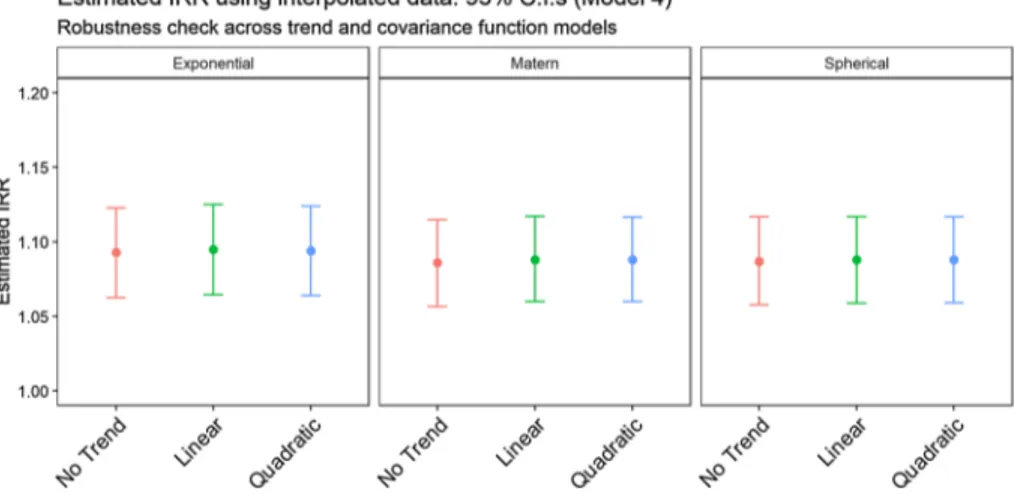
As previously anticipated, we re-estimate model (4) using different specifications of the Kriging interpolator. In particular, we first relax the mean-stationarity assumption of Ordi-nary Kriging by modelling the mean function of the process through both a linear and a quadratic trend in latitude and longitude. Next, we replace the simple Exponential function with a Spherical model and a more flexible Matérn kernel with the characteristic parameter set at 3/2 (to preserve mean-square differentiability). All these specifications still assume covariance stationarity. Figure 6 and Table 5 in the Appendix report the estimated Inci-dence Rate Ratios (IRR) regression coefficients for the PM variable in model (4) under these multiple setups: both point estimates and 95% confidence intervals indicate that there are no substantive differences between using different trend or covariance models, indicat-ing that our result is robust to alternative specification of the interpolation method.
Fig. 6 Robustness Check: estimated IRR (PM variable only) for PM in Model 4 using three different covar-iance functions and three alternative trend models
10 IRRs indicate the % change in Covid-related mortality for each one-unit increase in PM2.5
concentra-tion.
11 van Donkelaar, A., R. V. Martin, M. Brauer, N. C. Hsu, R. A. Kahn, R. C. Levy, A. Lyapustin, A. M.
Sayer, and D. M. Winker. 2018. Global Annual PM2.5 Grids from MODIS, MISR and SeaWiFS Aerosol Optical Depth (AOD) with GWR, 1998–2016. Palisades, NY: NASA Socioeconomic Data and Applications Center (SEDAC). https ://doi.org/10.7927/H4ZK5 DQS. Accessed 01 Mar 2020. See van Donkelaar et al. (2016) for further reference.
12 2016 Annual average concentration in μg/m3 of Pm 2.5 processed from the Data Integration Model for
Air Quality (DIMAQ) (Shaddick et al. 2018) from the WHO website.
13 Monitoring Air quality data for PM2.5 annual average concentration for 2016 and 2017, interpolated in a
4 Discussion
In each of the four specifications presented, the coefficient related to PM2.5 is always of the hypothesized direction and statistically different from zero. Precisely and consistently with pre-vious results for the original SARS-Coronavirus during the 2003 outbreak (Cui et al. 2003), an increase in air pollution exposure is associated with increased mortality for COVID-19. The first panel in Fig. 4, as well as Table 4, suggests that, when using interpolated data from ISPRA monitoring stations, the increase in mortality rate due to a one-unit increase in PM2.5 concentration varies between 14% (model 1—highest rate) and nearly 9% (model 4—lowest rate). The 95% confidence interval for the point estimate in model 4 lies between roughly 6% and 12%. Our findings fall in line with both Wu et al. (2020) and Cole et al. (2020) papers. Specifically, both papers find a positive ecological relationship between PM2.5 and COVID-19 mortality. In relation to a 1 µg/m3 increase in PM2.5, Wu et al. find 8% change in COVID-19 mortality, Cole et al. find the same increase associated to additional 3 COVID-COVID-19 deaths (almost 17% if compared to their sample mean), and our paper finds 9% increase in COVID-19 related excess mortality. Despite this similarity in results, the two key differences between our study and the others relate to the exposure assessment method and the outcome assessment method. In our study we use a spatial interpolation method (kriging) from ground-level moni-toring data, whereas these other two studies utilize PM2.5 gridded surfaces such as chemical transport modelling in the case of Cole et al. and a hybrid approach using chemical transport, aerosol optical depth and land use regression modelling in the case of Wu et al. With respect to COVID-19 mortality data, Wu et al. use county-level data from the Johns Hopkins Univer-sity, Center for Systems Science and Engineering Coronavirus Resource Center, which is com-prised of COVID-19 deaths tabulated by the US Centers for Disease Control and Prevention and State health departments. In Cole et al., researchers obtained COVID-19 deaths by resi-dential address and aggregated these to the municipality level. The obvious difference between their study and ours is that we used a surrogate excess mortality measure due to the issues of reliability for COVID-19 death data, as we have already discussed. The other relevant differ-ence between our study and the Wu et al. and Cole et al. studies is that we subsample the total cohort of Italian municipalities to only regions with a very high mortality rate, which are also the regions most affected by the air quality problems. On the other hand, when satellite data are used, our estimate yields lower incidence ratios. Although ground-level concentration metrics come with fewer measurement errors, satellite data proves nevertheless useful in corroborating both the direction and the significance of the effect of interest. This redundancy is particularly relevant in light of the relatively few stations capable of detecting the finest particulate.
With reference to model (4) and the remaining covariates, we observe no effect related to population density or income or the extent of industrial areas in the municipality. Like-wise, there is no evidence suggesting significant links between the share of non-EU resi-dents, the female to male ratio (which disappears after we incorporate the random effects), and the level of education (proxy by the percentage of university students) on the dependent variable of interest. On the other hand, our results suggest a negative association between temperatures and mortality due to COVID-19. Finally, as expected, we find that munici-palities with higher shares of the population aged 65 or more have been most affected. The distance from the closest airport, a measure of relational connectedness that also proxy for the exposure to the contagion process, deserves a last comment. We find that municipali-ties closer to an airport experience a higher number of deaths in excess. We speculate that
the result could be related to a higher likelihood for these municipalities to become clusters of contagion in the initial phase of the pandemic, but a causal link cannot be inferred based on our result ad the topic needs more research to be addressed adequately.
We conclude our analysis by checking the consistency of our results to different choices of the dependent variable. Existing evidence (Dominici et al. 2003; Pascal et al. 2014; Samet et al.
2000; Yin et al. 2017) associates fine PM to severe cardiovascular and respiratory diseases and mortality. In European cities, in particular, an estimated increase in the number of daily deaths of 0.7% is associated with an increase of 10 µg/m3 of PM
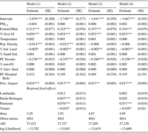
10 (Katsouyanni et al. 2001). This evidence suggests that long term PM exposure may have had an overall effect on deaths even before the outbreak in the sample municipalities, making it more difficult to isolate the real effect on COVID-19 deaths. We thus run model (4) using the total number of deaths in the same observation period of 2019 as the dependent variable to understand whether the effect of fine PM2.5 on mortality has been more severe during the pandemic. We find no evidence of an effect of PM2.5 on total deaths for 2019 in the sampled municipalities, suggesting that the effect of PM exposure on the mortality rate is closely connected to the novel coronavirus outbreak (see Table 6 in the Appendix). However, since the dependent variable in this “placebo” regres-sion cannot be directly compared to the excess mortality, we repeat the test using total mortality for the year 2020. Although the latter includes both COVID-19 related and unrelated deaths, these two variables represent data generating processes of the same nature. As expected, both the regression coefficients and IRRs calculated regressing total deaths in 2020 suggest a posi-tive and statistically significant effect of exposure to fine particulate on mortality, even though its magnitude is greatly reduced if compared to the estimates in Tables 3 and 4 (see Table 7 in the Appendix). Presumably, the effect of PM2.5 concentration on COVID-19 related mortality becomes muted by the noise introduced when accounting for other causes of death. This would also explain the non-significant PM2.5 coefficient in the first “placebo” regression.
5 Conclusion
Italy is among the countries most severely affected by the new coronavirus, with more than 230 thousand confirmed cases and more than 30 thousand deaths as of the end of May. Yet, the spatial distribution of confirmed cases and deaths suggest that the effects of the viral infection spreading largely vary across the regions of the country but also within regions. In this work, we examined the role of ambient PM2.5 in explaining the spatial variation in deaths that occurred throughout the most extreme time period of the epidemic. The results in the paper, that suggest a positive relationship between PM2.5 concentration and COVID-19 related excess mortality, are robust to different specifications PM2.5 and estimation strategies, even after controlling for additional confounder factors. Coherently with previous findings in the literature, we highlight a strong positive correlation between viral respiratory infection incidence and ambient PM2.5 concentrations and the increase in susceptibility to COVID-19 mortality caused by long term exposure to PM2.5, consistent with evidence for the original SARS-Coronavirus during the 2003 outbreak. In fact, fine PM is already known to affect car-diovascular and respiratory morbidity and mortality.
However, we are aware that the phenomenon and the cause and effect relationships are very complex and that our work can only address part of the problem. The cross-sec-tional nature of the dataset and the use of geographically aggregated information in the
epidemiological model does not allow concluding a causal effect exists. In our opinion, the robust evidence in the paper shows that the relationship between PM2.5 and COVID-19 related excess deaths goes far beyond a simple geographical correlation, and further research is needed to explore the causal effect more in depth, when reliable time series data are available.
In fact, our paper does not deal with the spread of contagion and the dynamics linked to it, also because, as we underlined, such analysis would require time-series data, a different econometric methodology, and the identification of the exogenous Coronavirus insurgence in Northern Italy. To the latter purpose, the spread of the pandemic incorporates two dif-ferent dynamics: (1) on the one hand, the dynamics of the spread of the contagion requires further information to be investigated such as its genesis, the type of virus, and setting of the first outbreak; (2) the effects of the lockdown changed (or partially blocked) the contagion in an asymmetric way. In addition to this, of course, there are other elements that should be investigated, such as additional variables about health data, mobility, and so forth.
Our results reinforce the need to adopt environmental policies that would not only reduce the impact of pollution on the health of citizens and workers but would contribute to smooth the negative effects of a (future) pandemics, avoiding collapses of health systems. Indeed, recent studies show that in addition to chronic lung inflammation, environmental air pollutant concen-trations can exacerbate the effects of increasingly frequent one-shot systemic shocks, which in turn are also caused by environmental factors. In this regard, sustainable and decarbonization policies such as the Green New Deal, conceived as long-term policies, should be accelerated.
Acknowledgements Open access funding provided by Università Cattolica del Sacro Cuore within the
CRUI-CARE Agreement. The authors would like to acknowledge the One Health Center of Excellence for having facilitated the research collaboration behind this work. The current version of the manuscript ben-efits of the shared reflection and comments on earlier drafts from the many colleagues at the OHC, among which Ilaria Capua, Olga Munoz and Elisa Pasqual, to whom the authors are grateful. The authors would also like to thank the editor and two ananymous referee for having provided very relevant suggestions. Any error or omission remains solely the author’s responsibility.
Open Access This article is licensed under a Creative Commons Attribution 4.0 International License,
which permits use, sharing, adaptation, distribution and reproduction in any medium or format, as long as you give appropriate credit to the original author(s) and the source, provide a link to the Creative Com-mons licence, and indicate if changes were made. The images or other third party material in this article are included in the article’s Creative Commons licence, unless indicated otherwise in a credit line to the material. If material is not included in the article’s Creative Commons licence and your intended use is not permitted by statutory regulation or exceeds the permitted use, you will need to obtain permission directly from the copyright holder. To view a copy of this licence, visit http://creat iveco mmons .org/licen ses/by/4.0/.
Appendix 1
Table 5 Estimated regression coefficient (PM variable only) for Model 4 using nine Kriging specifications: three different covariance functions (Exponential, Matérn and Spherical) time three alternative trend mod-els (constant trend, linear trend and quadratic trend)
The table also includes the estimated regression parameters for Model (4) using Satellite and EEA data
Method Covariance Trend Estimate Std. Err. p value AIC
Kriging Exponential No Trend 0.089 0.014 < 0.001 20,296
Linear 0.091 0.014 < 0.001 20,295 Quadratic 0.09 0.014 < 0.001 20,295 Matern No Trend 0.082 0.014 < 0.001 20,300 Linear 0.085 0.013 < 0.001 20,296 Quadratic 0.085 0.013 < 0.001 20,295 Spherical No Trend 0.083 0.014 < 0.001 20,300 Linear 0.084 0.014 < 0.001 20,298 Quadratic 0.084 0.014 < 0.001 20,298 Satellite MODIS 2016 – 0.02 0.01 0.013 20,329 DIMAQ 2016 – 0.02 0.01 0.068 20,331 DIMAQ 2014–2016 – 0.02 0.013 0.148 20,333 EEA 2016–2017 – 0.026 0.01 0.003 20,326
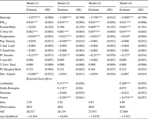
Table 6 Estimation results for the placebo regression, dependent variable: total number of deaths during the period Jan1-April 30 2019, municipalities in Northern Italy
***p < 0.01, **p < 0.05, *p < 0.1
Model (1) Model (2) Model (3) Model (4)
Estimate (SE) Estimate (SE) Estimate (SE) Estimate (SE)
Intercept − 5.072*** (0.806) − 5.209*** (0.760) − 5.530*** (0.812) − 5.809*** (0.790) PM2.5 0.044*** (0.003) 0.034*** (0.004) 0.033*** (0.005) 0.031*** (0.006) Female/Male − 0.034 (0.202) 0.304 (0.193) 0.669*** (0.193) 0.642*** (0.191) % Over 65 0.062*** (0.003) 0.061*** (0.003) 0.057*** (0.003) 0.057*** (0.003) Temperature − 0.018*** (0.003) − 0.013*** (0.003) − 0.014** (0.004) − 0.010* (0.004) Pop. Density − 0.010 (0.013) − 0.048*** (0.012) − 0.001 (0.012) − 0.008 (0.012) % Ind. Land − 0.004 (0.003) − 0.004 (0.002) − 0.004 (0.002) − 0.004 (0.002) % Samll Ent. − 0.003 (0.003) − 0.006 (0.003) − 0.002 (0.003) − 0.003 (0.003) PC Income − 0.215** (0.073) − 0.201** (0.069) − 0.217** (0.076) − 0.177* (0.074) % non-EU 0.006 (0.007) 0.009 (0.007) − 0.002 (0.007) 0.000 (0.007) % Univ. Stud. 0.000 (0.000) 0.000 (0.000) 0.000 (0.000) 0.000 (0.000) PC Hospital Beds 0.723 (0.904) 0.231 (0.863) 0.364 (0.827) 0.223 (0.825) Dist. Airport − 0.040** (0.012) − 0.014 (0.011) − 0.018 (0.016) − 0.007 (0.014)
Regional fixed effects
Lombardia 0.317*** (0.036) 0.289*** (0.055) Emila-Romagna 0.118** (0.04) 0.072 (0.057) Piemonte − 0.026 (0.035) − 0.023 (0.053) Veneto − 0.283*** (0.041) − 0.274*** (0.057) theta 3.29 3.92 4.87 4.89 Observations 4041 4041 4041 4041 AIC 28,517 28,119 27,971 27,869 log-Likelihood − 14,244 − 14,041 − 13,970 − 13,915
Appendix 2
See Table 6.Appendix 3
See Table 7.Appendix 4
Data comparison from different official sources.
Table 8 reports the excess deaths data as reported by the Italian Bureau of Statistics (ISTAT) along with the official covid19 statistics as indicated by Protezione Civile Italiana (PC). ED-I stands for Excess deaths reported by ISTAT, calculated as the sum of deaths (from all causes) between January 1 and March 31 (column 1) or April 30. 2020 (column 3) with respect to the average value in 2015–2019 (same months). The difference between column 1 and column 2 involves the sampling base. In fact, as long as ISTAT was upgrad-ing the deaths data, it was both enlargupgrad-ing the sample of municipalities and correctupgrad-ing the past figures; see column 4 to 6: TD-I (a) stands for Total deaths reported by ISTAT as the sum of total deaths from January 1 to March 31, 2020 in the initial sample (column 4),
Table 7 Estimation results for the placebo regression, dependent variable: total number of deaths during the period Jan1–April 30 2020, municipalities in Northern Italy
***p < 0.01, **p < 0.05, *p < 0.1
Model (1) Model (2) Model (3) Model (4)
Estimate (SE) Estimate (SE) Estimate (SE) Estimate (SE) Intercept − 3.876*** (0.280) − 3.748*** (0.277) − 3.641*** (0.295) − 3.667*** (0.292) PM2.5 − 0.001 (0.001) 0.000 (0.001) 0.000 (0.002) 0.002 (0.002) Female/Male 0.313*** (0.077) 0.325*** (0.076) 0.357*** (0.079) 0.354*** (0.079) % Over 65 0.056*** (0.001) 0.054*** (0.001) 0.053*** (0.001) 0.053*** (0.001) Temperature 0.002 (0.001) 0.001 (0.001) 0.001 (0.001) 0.000 (0.001) Pop. Density − 0.014*** (0.003) − 0.012*** (0.003) − 0.006 (0.003) − 0.006 (0.003) % Ind. Land − 0.002* (0.001) − 0.002** (0.001) − 0.002** (0.001) − 0.002** (0.001) % Samll Ent. 0.001 (0.001) 0.000 (0.001) 0.001 (0.001) 0.000 (0.001) PC Income − 0.238*** (0.025) − 0.247*** (0.026) − 0.260*** (0.028) − 0.258*** (0.028) % non-EU 0.000 (0.002) 0.002 (0.002) 0.002 (0.003) 0.002 (0.003) % Univ. Stud. 0.000 (0.000) 0.000 (0.000) 0.000 (0.000) 0.000 (0.000) PC Hospital Beds 0.433 (0.365) 0.349 (0.362) 0.469 (0.354) 0.439 (0.355 Dist. Airport 0.016*** (0.004) 0.017*** (0.004) 0.017** (0.005) 0.017*** (0.005)
Regional fixed effects
Lombardia 0.013 (0.013) 0.002 (0.019) Emila-Romagna 0.047*** (0.013) 0.028 (0.019) Piemonte 0.076*** (0.013) 0.071*** (0.018) Veneto − 0.035* (0.014) − 0.039* (0.02) theta 3.29 3.92 4.87 4.89 Observations 4041 4041 4041 4041 AIC 27,432 27,327 27,269 27,238 log-Likelihood − 13,702 − 13,645 − 13,619 − 13,600
Table 8 R egional com par ison of deat h dat a fr om differ ent sour ces ED-I (a) ex cess deat hs r epor ted b y IS TA T Januar y 1-Mar ch 31 2020 wit h initial sam ple; ED-I (b) ex cess deat hs b y IS TA T Januar y 1-Mar ch 31 wit h enlar ged sam ple; ED-I (c) ex cess deat hs b y IS TA T, lates t r elease; TD-I (a) to tal deat hs b y IS TA T Januar y 1-Mar ch 31 wit h initial sam ple; D-PC number of deat hs wit h or fr om Co vid-19 r egis ter ed b y Pr otezione Civile It aliana (PC). T ot al municipalities in N or ther n It aly : 7904 Regions (1) (2) (3) (4) (5) (6) (7) (8) (9) (10) (11) ED-I (a) 1 J-31 M ED-I (b) 1 J-31 M ED-I (c) 1 J-30A TD-I (a) 1 J-31 M TD-I (b) 1 J-31 M TD-I (c) 1 J-30A D-PC 31 M D-PC 30A (1)/(7) (2)/(7) (3)/(8) Emilia- Romagna 1874 3251.5 4525 8433 16,879 22,142 1644 3551 1.14 1.98 1.27 Fr iuli-Venezia Giulia 44 55 255 353 1596 5332 113 289 0.39 0.49 0.88 Ligur ia 65 837.75 1454 3982 6187 9193 428 1167 0.15 1.96 1.25 Lombar dy 8539 15,771.75 23,329 26,749 40,969 58,882 7199 13,772 1.19 2.19 1.69 Piemonte 816 2216.75 3547 5566 12,637 21,931 854 3066 0.96 2.60 1.16 Tr entino-Alt o Adig e 132 416.25 1048 551 1737 4286 240 693 0.55 1.73 1.51 Valle d’ Aos ta 25 117 128 184 541 622 56 137 0.45 2.09 0.93 Vene to 529 1002 1723 4884 12,645 18,248 477 1459 1.11 2.10 1.18 tot al 12,024 23,668 36,009 50,702 93,191 140,636 11,011 24,134 1.09 2.15 1.49 municipalities n.a. 6866 7270 n.a. 6866 7270 – – – – –
TD-I (b) for the updated sample (column 5) and TD-I (c) for the latter release. It turned out that the number of ISTAT excess deaths increased by 97% with this revision (compare column 1 and column 2). It further increased by 52% on April 30 (compare column 2 and column 3) due to corrections, enlargement and new cases.
D-PC stands for number of deaths with or from Covid-19 reported by the national department Protezione Civile Italiana (Italian Civil Protection, which is a department of the Presidency of the Italian Council of Ministers) over January 1-March 31, 2020 (column 7) and January 1-April 30, 2020 in column 8. The official D-PC data are available only at the regional level and they are officially released by the health departments of the Regional administrations. In the period March 31 and April 30, PC registered a 119% increase in Covid-19 deaths.
ISTAT and PC department therefore collect data independently. The key difference between ED-I and D-PC lies in how PC recognizes fatalities as Covid-19 related: only patients known to have tested positive to SARS-COV-2 got registered under this nomen-clature. On the other hand, ED-I is just a mathematical construct that takes into account all deaths in a given municipality, regardless the cause. Due to difficulties in providing timely screenings and accurate testing during the peak of the pandemics, it is likely that official figures from PC might have been underestimated between early January and mid-April. This is particularly true for the most affected areas. Consequently, the discrepancies between ED-I and D-PC can be either moderate or strong, as we observe for Lombardy (where ED-I is roughly 69% higher than D-PC) and Trentino Alto-Adige. Last, the unlikely event of ED-I lying below D-PC is due the fact that ISTAT initially collected figures for only a subsample of municipalities (i.e. those recording a percentage of excess deaths in 2020 greater than 20%) leaving out quite a lot of statistical units (for example, Friuli-Vene-zia Giulia, which had initially the biggest discrepancy (ratio 0,39) reported data for a very small number of municipalities to ISTAT). However, with some delay, ISTAT has been upgrading the sample, such that in June it covered about all municipalities.
In our paper, we use the updated data ED-I 1 J-30A (column 3), disaggregated at the municipality level. Column (9) shows that the ratio of total ED-I and D-PC is about 1.09, with mean ratio equal to 0.74 and standard deviation equal to 0.4. Underestimation of cases in the initial sampling base concerned all Northern Italian regions except Emilia Romagna, Lombardy and Veneto (the biggest regions in terms of population and Covid-19 cases).
The ratio of total ED-I (b) and D-PC (b) in column (10) is about 2.1, with a mean ratio equal to 1.89 and standard deviation 0.6. One month later, the total ratio decreases to 1.5— column (11)—with mean ratio 1.24 and standard deviation 0.27. In the latter case, a slight underestimation of the registered cases concerns only FVG and Valle d’Aosta.
In any case, since Lombardy has the biggest discrepancy on April 30 (ratio 1,69) we also run our regressions excluding Lombardy (i.e. taking all Lombardy municipalities off) and the results are robust, reporting a significant higher-than-1 relative risk ratio for the exposure variable. The latter results are available upon request.
References
Becattini G (2002) From Marshall’s to the Italian “industrial districts”. A brief critical reconstruction. In: Contributions to Economics, pp 83–106. https ://doi.org/10.1007/978-3-642-50007 -7_6
Becchetti L, Conzo G, Conzo P, Salustri F (2020) Understanding the heterogeneity of adverse COVID-19 outcomes : the role of poor quality of air and lockdown decisions. SSRN 3572548
Bigi A, Ghermandi G (2016) Trends and variability of atmospheric PM 2.5 and PM 10–2.5 concentration in the Po Valley, Italy. Atmos Chem Phys 16(24):15777–15788. https ://doi.org/10.5194/acp-16-15777 -2016
Bivand RS, Pebesma E, Gómez-Rubio V (2013) Applied spatial data analysis with R. Springer, New York.
https ://doi.org/10.1007/978-1-4614-7618-4
Bowe B, Xie Y, Yan Y, Al-Aly Z (2019) Burden of Cause-Specific Mortality Associated With PM 2.5 Air Pollution in the United States. JAMA Netw Open 2(11):e1915834. https ://doi.org/10.1001/jaman etwor kopen .2019.15834
Brandt EB, Beck AF, Mersha TB (2020) Air pollution, racial disparities, and COVID-19 mortality. J Allergy Clin Immunol 146(1):61–63. https ://doi.org/10.1016/j.jaci.2020.04.035
Cakmak S, Hebbern C, Pinault L, Lavigne E, Vanos J, Crouse DL, Tjepkema M (2018) Associations between long-term PM2.5 and ozone exposure and mortality in the Canadian Census Health and Environment Cohort (CANCHEC), by spatial synoptic classification zone. Environ Int 111:200– 211. https ://doi.org/10.1016/j.envin t.2017.11.030
Carugno M, Consonni D, Randi G, Catelan D, Grisotto L, Bertazzi PA, Biggeri A, Baccini M (2016) Air pollution exposure, cause-specific deaths and hospitalizations in a highly polluted Italian region. Environ Res 147:415–424. https ://doi.org/10.1016/j.envre s.2016.03.003
Ciencewicki J, Jaspers I (2007) Air pollution and respiratory viral infection. Inhal Toxicol 19(14):1135– 1146. https ://doi.org/10.1080/08958 37070 16654 34
Ciminelli G, Garcia-mandicó S (2020) 19 in Italy: an analysis of Death Registry Data COVID-19 in Italy. https ://voxeu .org/artic le/covid -19-italy -analy sis-death -regis try-data. Accessed 22 Apr 2020
Cole MA, Ozgen C, Strobl E (2020) Air pollution exposure and COVID-19. IZA Discussion Paper Series, 13367
Conticini E, Frediani B, Caro D (2020) Can atmospheric pollution be considered a co-factor in extremely high level of SARS-CoV-2 lethality in Northern Italy? Environ Pollut. https ://doi.org/10.1016/j. envpo l.2020.11446 5
Cui Y, Zhang Z-F, Froines J, Zhao J, Wang H, Yu S-Z, Detels R (2003) Air pollution and case fatality of SARS in the People’s Republic of China: an ecologic study. Environ Health 2(1):1–5. https ://doi. org/10.1186/1476-069x-2-15
Dominici F, McDermott A, Zeger SL, Samet JM (2003) Airborne particulate matter and mortality: time-scale effects in four US cities. Am J Epidemiol 157(12):1055–1065. https ://doi.org/10.1093/aje/ kwg08 7
Eeftens M, Tsai M-Y, Ampe C, Anwander B, Beelen R, Bellander T, Cesaroni G, Cirach M, Cyrys J, de Hoogh K, De Nazelle A, de Vocht F, Declercq C, Dėdelė A, Eriksen K, Galassi C, Gražulevičienė R, Grivas G, Heinrich J et al (2012) Spatial variation of PM2.5, PM10, PM2.5 absorbance and PMcoarse concentrations between and within 20 European study areas and the relationship with NO2—results of the ESCAPE project. Atmos Environ 62:303–317. https ://doi.org/10.1016/j.atmos
env.2012.08.038
European Environmental Agency (2019) Air quality in Europe—2019 report—EEA Report No 10/2019 (Issue 10). https ://doi.org/10.2800/82235 5
Giulianelli L, Gilardoni S, Tarozzi L, Rinaldi M, Decesari S, Carbone C, Facchini MC, Fuzzi S (2014) Fog occurrence and chemical composition in the Po valley over the last twenty years. Atmos Envi-ron 98:394–401. https ://doi.org/10.1016/j.atmos env.2014.08.080
Goutte S, Péran T, Porcher T (2020) The role of economic structural factors in determining pandemic mortality rates: evidence from the COVID-19 outbreak in France. Res Int Bus Financ 54:101281.
https ://doi.org/10.1016/j.ribaf .2020.10128 1
Horálek J, Schreiberová M, de Leeuw F, Kurfürst P, de Smet P, Schovánková J (2018) European air quality maps for 2016, Eionet Report-ETC/ACM 2018/8
Istituto Superiore di Sanità (2020) Characteristics of COVID-19 patients dying in Italy Report based on available data on March 20 th, 2020. 4–8
Jeong S-C, Cho Y, Song M-K, Lee E, Ryu J-C (2017) Epidermal growth factor receptor (EGFR)-MAPK-nuclear factor(NF)-κB-IL8: a possible mechanism of particulate matter(PM) 2.5-induced lung tox-icity. Environ Toxicol 32(5):1628–1636. https ://doi.org/10.1002/tox.22390
Katsouyanni K, Touloumi G, Samoli E, Gryparis A, Le Tertre A, Monopolis Y, Rossi G, Zmirou D, Bal-lester F, Boumghar A, Anderson HR, Wojtyniak B, Paldy A, Braunstein R, Pekkanen J, Schindler C, Schwartz J (2001) Confounding and effect modification in the short-term effects of ambient par-ticles on total mortality: results from 29 European cities within the APHEA2 project. Epidemiology 12(5):521–531. https ://doi.org/10.1097/00001 648-20010 9000-00011
Larsen BR, Gilardoni S, Stenström K, Niedzialek J, Jimenez J, Belis CA (2012) Sources for PM air pollution in the Po Plain, Italy: II. Probabilistic uncertainty characterization and sensitivity analysis of second-ary and primsecond-ary sources. Atmos Environ 50:203–213. https ://doi.org/10.1016/j.atmos env.2011.12.038
ARPA Lombardia (2020) Analisi preliminare della qualità dell’ aria in Lombardia durante l’ emergenza COVID-19. https ://www.arpal ombar dia.it/Pages /Quali tà-dell’aria-duran te-l’emerg enza-Covid -19,-l’anali si-di-Arpa-Lomba rdia-.aspx. Accessed 03 Apr 2020
Ma Y, Zhao Y, Liu J, He X, Wang B, Fu S, Yan J, Niu J, Zhou J, Luo B (2020) Effects of temperature variation and humidity on the death of COVID-19 in Wuhan, China. Sci Total Environ 724:138226.
https ://doi.org/10.1016/j.scito tenv.2020.13822 6
McGuinn LA, Ward-Caviness C, Neas LM, Schneider A, Di Q, Chudnovsky A, Schwartz J, Koutrakis P, Russell AG, Garcia V, Kraus WE, Hauser ER, Cascio W, Diaz-Sanchez D, Devlin RB (2017) Fine particulate matter and cardiovascular disease: comparison of assessment methods for long-term exposure. Environ Res 159(July):16–23. https ://doi.org/10.1016/j.envre s.2017.07.041
Moran PAP (1950) Notes on continuous stochastic phenomena. Biometrika 37:17–23
Mukherji N (n.d.) The social and economic factors underlying the incidence of COVID-19 cases and deaths in US counties. MedRxiv, 2020.05.04. https ://doi.org/10.1101/2020.05.04.20091 041
Odone A, Delmonte D, Scognamiglio T, Signorelli C (2020) COVID-19 deaths in Lombardy, Italy: data in context. Lancet Publ Health 2667(20):30099. https ://doi.org/10.1016/S2468 -2667(20)30099 -2
Ogen Y (2020) Assessing nitrogen dioxide (NO2) levels as a contributing factor to coronavirus (COVID-19) fatality. Sci Total Environ 726:138605. https ://doi.org/10.1016/j.scito tenv.2020.13860 5
Pascal M, Falq G, Wagner V, Chatignoux E, Corso M, Blanchard M, Host S, Pascal L, Larrieu S (2014) Short-term impacts of particulate matter (PM10, PM10-2.5, PM2.5) on mortality in nine French cities. Atmos Environ 95:175–184. https ://doi.org/10.1016/j.atmos env.2014.06.030
Pirovano G, Colombi C, Balzarini A, Riva GM, Gianelle V, Lonati G (2015) PM2.5 source apportionment in Lombardy (Italy): comparison of receptor and chemistry-transport modelling results. Atmos Envi-ron 106:56–70. https ://doi.org/10.1016/j.atmos env.2015.01.073
Pozzer A, Bacer S, Sappadina SDZ, Predicatori F, Caleffi A (2019) Long-term concentrations of fine par-ticulate matter and impact on human health in Verona, Italy. Atmos Pollut Res 10(3):731–738. https :// doi.org/10.1016/j.apr.2018.11.012
Samet JM, Dominici F, Curriero FC, Coursac IMS, Zeger SL (2000) Fine particulate air pollution and mor-tality in 20 U.S. Cities, 1987-1994. N Engl J Med 343(24):1742–1749. https ://doi.org/10.1056/NEJM2 00104 19344 1614
Sedlmaier N, Hoppenheidt K, Krist H, Lehmann S, Lang H, Büttner M (2009) Generation of avian influ-enza virus (AIV) contaminated fecal fine particulate matter (PM2.5): genome and infectivity detec-tion and calculadetec-tion of immission. Vet Microbiol 139(1–2):156–164. https ://doi.org/10.1016/j.vetmi c.2009.05.005
Setti L, Passarini F, de Gennaro G, Di Gilio A, Palmisani J, Buono P, Fornari F, Grazia Perrone M, Piaz-zalunga A, Pierluigi B, Rizzo E, Miani A (2020) Evaluation of the potential relationship between Par-ticulate Matter (PM) pollution and COVID-19 infection spread in Italy. SIMA Position Paper. http:// www.simao nlus.it/wpsim a/wp-conte nt/uploa ds/2020/03/COVID _19_posit ion-paper _ENG.pdf
Shaddick G, Thomas ML, Green A, Brauer M, van Donkelaar A, Burnett R, Chang HH, Cohen A, Van Dingenen R, Dora C, Gumy S, Liu Y, Martin R, Waller LA, West J, Zidek JV, Prüss-Ustün P (2018) Data integration model for air quality: a hierarchical approach to the global estimation of exposures to ambient air pollution. J Royal Stat Soc: Ser C (Appl Stat) 67(1):231–253
Shi Y, Wang Y, Shao C, Huang J, Gan J, Huang X, Bucci E, Piacentini M, Ippolito G, Melino G (2020) COVID-19 infection: the perspectives on immune responses. Cell Death Differ. https ://doi. org/10.1038/s4141 8-020-0530-3
van Donkelaar A, Martin RV, Brauer M, Hsu NC, Kahn RA, Levy RC, Lyapustin A, Sayer AM, Winker DM (2016) Global estimates of fine particulate matter using a combined geophysical-statistical method with information from satellites. Environ Sci Technol 50(7):3762–3772. https ://doi.org/10.1021/acs. est.5b058 33
Wu X, Nethery RC, Sabath BM, Braun D, Dominici F (2020) Exposure to air pollution and COVID-19 mor-tality in the United States. MedRxiv, 2020.04.05.20054502. https ://doi.org/10.1101/2020.04.05.20054 502
Yin P, Brauer M, Cohen A, Burnett RT, Liu J, Liu Y, Liang R, Wang W, Qi J, Wang L, Zhou M (2017) Long-term fine particulate matter exposure and nonaccidental and cause-specific mortality in a large national cohort of Chinese men. Environ Health Perspect 125(11):117002. https ://doi.org/10.1289/ EHP16 73
Yorifuji T, Kashima S, Tani Y, Yamakawa J, Doi H (2019) Long-term exposure to fine particulate mat-ter and natural-cause and cause-specific mortality in Japan. Environ Epidemiol 3(3):e051. https ://doi. org/10.1097/EE9.00000 00000 00005 1
Publisher’s Note Springer Nature remains neutral with regard to jurisdictional claims in published maps and institutional affiliations.