Analysis of Wiener phase noise issues in optical transmission systems

(1)

POLITECNICO DIMILANO

DEPARTMENT OFELECTRONICS, INFORMATION, AND

BIOENGINEERING

DOCTORALPROGRAMME IN INFORMATIONENGINEERING

A

NALYSIS OF

W

IENER

P

HASE

N

OISE

I

SSUES IN

O

PTICAL

T

RANSMISSION

S

YSTEMS

Doctoral Dissertation of:

Silvio Mandelli

Supervisor:

Prof. Maurizio Magarini

Tutor:

Prof. Andrea Virgilio Monti Guarnieri

The Chair of the Doctoral Program:

Prof. Carlo Fiorini

(2)

(3)

Abstract

I

N optical communications, local oscillators and propagation introduce multiplicative phase noise that must be taken in consideration, esti-mated and compensated at the receiver. In the literature such channels are dealt with by considering a symbol-spaced discrete-time model where the transmitted symbol is impaired by both AWGN and a multiplicative phase noise given by a first order Wiener process. The issues given by such channels are objects of several works in the literature. The aim of this thesis is to discuss some of them and try to extend those dissertations.

First of all, in the literature this model is assumed by considering “small” phase noise but nobody has ever discussed how much “small” it must be. A statistical and mathematical analysis is derived by the author, and a thresh-old of validity of the so called Discrete Model is worked out, proving that the assumption is correct in almost all practical scenario and it is conserva-tive in term of performance simulation. The analysis of phase noise chan-nels is then deepened by studying Bayesian tracking techniques to extract all the information about the transmitted symbols. An iterative demod-ulation and decoding scheme is proposed and compared to others in the literature. The major gain is given by the greater spectral efficiency ob-tained by not transmitting Pilot Symbols and still working better than other considered similar schemes. Bayesian tracking allows also to derive the in-formation rate of the considered Discrete Model channel and to verify that the proposed algorithm can achieve it.

The focus is then moved to analyze short reach access optical scenarios where, for spectral efficiency and receiver sensitivity, OFDM has been

(4)

sidered instead of single carrier systems. For cost, footprint and power con-sumptions requirements, Direct Detection has several advantages compared to Coherent schemes since the multiplicative phase noise introduced by the transmitting laser can be neglected. However, if dispersive compensating fibers are not used, Chromatic Dispersion impairs the signal and the phase noise cannot be canceled. The author has proposed the literature analysis of this phenomenon, enlightening its weaknesses and comparing the new re-sults of the thesis with experimental measurements given by other authors.

(5)

List of Figures

2.1 Complex baseband representation of the transmission sys-tem with multiplicative phase noise, matched filtering, and symbol-rate sampling. . . 10 2.2 Simulator Block Diagram for generating ηi, φi and φ′i. . . . 15

2.3 PCCˆ 1versus σPN for QPSK and 16-QAM. . . 16

2.4 PCCˆ 2versus σPN for QPSK and 16-QAM. . . 17

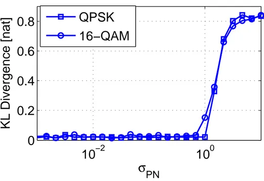
2.5 Kullback-Leibler Divergence versus σPNwith QPSK and

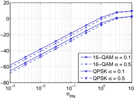
16-QAM. . . 19 2.6 Model Mismatch Power P between CM and DM versus σPN

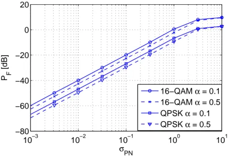
with QPSK and 16-QAM. . . 21 2.7 Model Mismatch Power PF between CM and the Filtered

DM versus σPN with QPSK and 16-QAM. . . 22

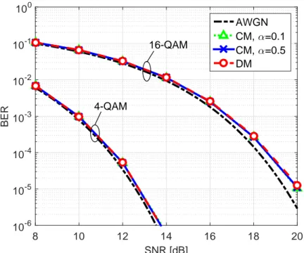
2.8 BER versus SNR with QPSK and 16-QAM with σPN = 3·

10−2 with QPSK and 16-QAM. . . 23 2.9 BER versus SNR with QPSK and 16-QAM with σPN = 6.6·

10−2 with QPSK and 16-QAM. . . 24

2.10 BER versus SNR with QPSK and 16-QAM with σPN =

0.135 with QPSK and 16-QAM. . . . 25 2.11 PSD of φi and φ′i of DM and CM respectively with σPN =

6.6· 10−2. . . 26 2.12 PSD of φi and φ′i of DM and CM respectively with σPN =

(8)

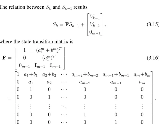
3.1 Block diagram of the sinusoid embedded in noise and af-fected by ARMA phase noise with order m = 1, i.e. Wiener Phase Noise. . . 35 3.2 Power spectral density of phase noise generated by

accumu-lating white Gaussian noise with zero mean and unit vari-ance (σ = 1) filtered through a causal, monic, and minimum phase transfer function. Solid line: phase noise model of the free-running oscillator in synchronization problems, re-ported in [Spalvieri and Magarini, 2008]. Dash-dotted line: phase noise generated by (3.21) with m = 4 followed by accumulation. Dashed line: Wiener’s phase noise. Dotted line: white phase noise. . . 37 3.3 ARMA phase noise example generated by (3.21) with m =

4 and σ = 1. . . . 38 3.4 Wiener’s phase noise example with σ = 1. . . . 38 3.5 Example of two-step Bayesian recursion applied to the

track-ing of the phase of the sinusoid embedded in noise affected by Wiener’s phase noise. SNR = 1dB, σ = 1, and p(s0) =

δ(s0). Dashed line: predictive distribution p(sk|y1k−1). Solid

line: posterior distribution p(sk|yk1). Asterisk: actual value

of the phase. (a) k = 1. (b) k = 2. (c) k = 3. (d) k = 4. . . 41 3.6 Example of MAP estimation applied to the phase tracking

of a sinusoid embedded in noise affected by Wiener’s phase noise. Specifically, the estimation is obtained by the maxi-mization of the posterior probability of the Bayesian recur-sion. SNR = 5dB, σ = 2, and p(s0) = δ(s0). Dashed line:

MAP estimation of the phase sk. Solid line: actual phase sk. 42

3.7 Example of forward-backward Bayesian recursion applied to the tracking of the wrapped phase of the sinusoid embed-ded in noise affected by Wiener’s phase noise. SNR = 8dB,

σ = 0.5, and n = 100. p(s0) and p(s101) are Dirac

func-tion. Grayscale image: probabilities distribution for each

k time indexes in the x-axis. White dots: actual value of

the phase. (a) forward predictive distribution p(sk|yk1−1).

(b) backward predictive distribution p(sk|yk+1n ). (c) forward

posterior distribution p(sk|y1k). (d) backward posterior

dis-tribution p(sk|ynk). (e) forward-backward distribution p(sk|y1n).

. . . 47 3.8 Block diagram of the Kalman filter. . . 50

(9)

3.9 Tikhonov distribution for different values of the parameter a. Solid line: a = exp(jπ/2). Dashed line: a = 0.5 exp(jπ). Dash-dotted line: a = 2 exp(j3π/2) . . . . 52 3.10 Examples of parametric Bayesian tracking by Tikhonov

ap-proximation for the phase tracking problem of a sinusoid affected by Wiener’s phase noise. σ = 0.5, SNR = 1dB,

p(s0) = (2π)−1. Solid line: actual posterior distribution

p(sk|y1k). Dashed line: actual predictive distribution p(sk|y1k−1).

Dash-dotted line: approximated posterior distribution t(sk, ak)

by Tikhonov parametrization. Dotted line: approximated predictive t(sk, ak) distribution by Tikhonov

parametriza-tion. Asterisk: actual value of the phase sk. (a) k = 1,

Tikhonov tracking with prediction rule in (3.65). (b) k = 1, Tikhonov tracking with prediction rule in (3.66). (c) k = 2, Tikhonov tracking with prediction rule in (3.65). (d) k = 2, Tikhonov tracking with prediction rule in (3.66). (e) k = 3, Tikhonov tracking with prediction rule in (3.65). (f) k = 3, Tikhonov tracking with prediction rule in (3.66). . . 55 3.11 Example of state diagram (left) and trellis digram (right) of

a finite state machine. . . 56 3.12 Example of forward Bayesian recursion by state-space

quan-tization applied to the tracking of the wrapped phase of the sinusoid embedded in noise affected by Wiener’s phase noise. SNR = 1dB, σ = 0.3, and |S| = 8. p(s0) is a Dirac

func-tion. (a) Grayscale image: forward posterior distribution

p(sk|y1k) approximated by state-space quantization; solid white

line: actual phase evolution. (b) Dotted line: MAP estima-tion from the forward posterior distribuestima-tion p(sk|yk1)

approx-imated by state-space quantization; solid black line: actual phase evolution. . . 58 3.13 Example of forward Bayesian recursion by particle filtering

applied to the tracking of the unwrapped phase of the si-nusoid embedded in noise affected by ARMA phase noise. SNR = 0dB, ARMA phase noise generated by (3.21) with

m = 4 and σ = 1, and p(ϕ0) uniform between [0, 2π).

Num-ber of particles P = 1000. Solid line: posterior distribution

p(ϕk|y1k) by formula (3.83) with σp2 = 0.1. Crosses: actual

phase. Dots on the x-axis: values of the first entry of the particles (ϕ(i)_k ) (a) k = 1. (b) k = 2. (c) k = 3. (d) k = 4. . 66

(10)

3.14 Block Scheme of the State-based Approach of a two sections optic channel. . . 69 3.15 Frequency and Impulse Responses of approximated

Square-Root Raised Cosine by m-th order transfer functions. (a)

m = 4 Impulse Response. (b) m = 4 Frequency Response.

(c) m = 5 Impulse Response. (d) m = 5 Frequency Re-sponse. (e) m = 6 Impulse ReRe-sponse. (f) m = 6 Frequency Response. . . 72 3.16 Phase Response of hCD(z), with z0 = 0.993ej2π·0.5/32 (solid

line) and its quadratic MMSE approximation (dashed). . . . 73 3.17 Block Scheme of the State-based Approach of a two sections

optic channel with additive noise at each fiber section. . . . 74 4.1 UB and LB of the information rate transferred through a DM

channel with QPSK transmission. . . 91 4.2 Proposed Iterative Demodulation and Decoding Algorithm

Block Scheme. . . 94 4.3 Achievable information rate versus σPN for the phase noise

channel with 16-QAM and two values of SNR. Dashed line: pure AWGN. Solid line with squares: full trellis, forward data-aided recursion. Dash-dotted line: full trellis with forward-backward non-data-aided recursions. Solid line: reduced complexity trellis with forward-backward non-data-aided re-cursions. . . 99 4.4 Achievable information rate versus σPN for the phase noise

channel with 64-QAM and two values of SNR. Dashed line: pure AWGN. Solid line with squares: full trellis, forward data-aided recursion. Dash-dotted line: full trellis with forward-backward non-data-aided recursions. Solid line: reduced complexity trellis with forward-backward non-data-aided re-cursions. . . 100 4.5 BER versus SNR. Dashed line: performance limit of AWGN

channel. Dash-dotted line: performance limit of AWGN and phase noise channel. Dashed line with triangles: pure AWGN. Solid line: hybrid iterative demodulation and de-coding without pilot symbols. Dotted line with crosses: full trellis with dataaided forward recursion and non-data-aided backward recursion. Solid line with circles: iterative de-modulation and decoding of Kamiya and Sasaki [Kamiya and Sasaki, 2013] with pilot rate 1/25. . . 102

(11)

5.1 OFDM Transmission and different delays due to Chromatic Dispersion. . . 105 5.2 Effects of the PN on the received subcarrier signal: (1-red)

power degradation α, (2-green) phase rotation term (PRT), and (3-brown) inter-carrier interference (ICI). . . 106 5.3 Effect on PRT’s statistic due to the sampling of the Phase

Noise PSD. . . 111 5.4 Received 16-QAM constellation transmitted over a L km

fiber in the SA model. . . 112 5.5 MSE of the received signal with the SA and MC simulator. . 113 5.6 DDO-OFDM Monte Carlo Simulator Block Scheme . . . . 114 5.7 MC Bit Error Rate versus L. SNR = 20 dB . . . 117

(12)

(13)

List of Tables

1.1 Iterations performed by the proposed hybrid iterative de-modulation and decoding algorithm. . . 8 4.1 Simulation Parameters of Trellis-based demodulation . . . . 98 5.1 Semi-Analytical (SA) DDO-OFDM transmission

(14)

(15)

List of Acronyms

AM Amplitude Modulation

ARMA AutoRegressive Moving Average

AWGN Additive White Gaussian Noise BCJR Bahl-Cocke-Jelinek-Raviv BER Bit Error Rate

CM Complete Model

DFB Distributed Feedback Lasers DM Discrete-time Model

DSB Dual Side-Band

DSP Digital Signal Processing

DTFN Discrete-Time Frequency Noise GVD Group-Velocity Dispersion FFT Fast Fourier Transform FSM Finite State Machine ICI Inter-Carrier Interference

(16)

ISI Inter Symbol Interference KLD Kullback-Leibler Divergence

LB Lower Bound

MIMO Multiple-In Multiple-Out

MMSE Minimum Mean Square Error

MC Monte Carlo

MSE Mean Square Error

p.d.f. probability density function PN Phase Noise

PCC Pearson’s Correlation Coefficient PD Power Degradation

PN Phase Noise

PRT Phase Rotation Term PSD Power Spectral Density

QAM Quadrature Amplitude Modulation SA Semi-Analytic

SER Symbol Error Rate SNR Signal-to-Noise Ratio SPN Small Phase Noise

SRRC Square-Root Raised Cosine SSB Single Side-Band

UB Upper Bound

VCSEL Vertical Cavity Surface Emitting Lasers ZP Zero-Padding

(17)

CHAPTER

1

Introduction

1.1

Background

Multiplicative phase noise is one of the major impairments affecting the performance of coherent optical transmission systems [Leoni et al., 2012, Magarini et al., 2012a, Goebel et al., 2011]. Phase noise is due to both laser oscillators used for up- and down-conversion [Foschini and Vannucci, 1988], and to cross-phase modulation that arises in wavelength-division-multiplexing systems [Essiambre et al., 2010]. In particular, in [Magarini et al., 2011], it is concluded that the discrete symbol-spaced Optical Chan-nels transmission can be modeled, if the phase noise line-width is “small”, as follows

yi = aiejφi+ ni , (1.1)

where ai is the transmitted complex symbol, φi a discretized first-order

Wiener process and ni AWGN. Several schemes have been proposed to

es-timate the received carrier phase for arbitrary PSK and QAM constellations in presence of phase noise. In this thesis work Bayesian Inference will be considered to analyze the features and deal with Equation (1.1) channel. In particular, Bayesian tracking is exploited to follow the hidden phase φi,

(18)

Tracking the state of a dynamic system from noisy measurements is a classical problem in several fields of science. In the state-space approach to time-series modeling, the state process describes all relevant informa-tion about the system under investigainforma-tion. For example, this informainforma-tion could be related to the kinematic characteristics of a generic target [Li and Jilkov, 2003, Blackman, 2004]. In an econometrics problem it could be re-lated to the interest rates or the monetary flow [Gray, 1996, Duffie, 2010]. Alternatively, it could be related to the motion characteristics in video an-alytics applications for visual tracking, where the aim is to automatically understand the actions occurring in a monitored scene [Isard and Blake, 1998, Kwon and Lee, 2010, Zhou et al., 2004, Ross et al., 2008].

In order to make inference about the state of a dynamic system that changes over time, a model of the state evolution with time (the system model) and a model related to the noisy measurements to the state (the mea-surement model) are required. For dynamic state estimation, the discrete-time approach is widespread and convenient. In the Bayesian approach, system and measurement models are available in a probabilistic form. Ac-cordingly, probabilities are used to model the state evolution and the mea-surement given the state, and, from the model and the meamea-surements, infer-ence is made on the hidden evolving state. By making inferinfer-ence one builds the probability of the state given all the available measurements, thus em-bodying all the available statistical information in the inferred distribution. Therefore it can be said that, in some sense, Bayesian tracking extracts the information about the state that is brought by the measurements. This provides a rigorous general framework for dynamic state estimation prob-lems [Simon, 2006].

The most popular tool for Bayesian tracking of a system with discrete-time continuous state is the Kalman filter proposed in [Kalman, 1960] (see, e.g., [Simon, 2006, Haykin, 2004], two comprehensive books on the Kalman filter). The Kalman filter performs optimal tracking, thus leading to exact inference, when the equations that describe the system model and the measurement model are linear and the noisy processes that affect the state evolution and the measurements are additive and independent Gaussian processes. When the state transition and/or the measurement equations are non-linear and/or the noise processes are non-Gaussian, the Kalman filter is no more optimal. To face the non-optimality of the Kalman filter in case of non-linear state model and/or measurement model, the extended Kalman filter has been proposed in [Bellantoni and Dodge, 1967] and adopted in more applications: real-time traffic estimation [Wang and Papageorgiou, 2005], data-assimilation in oceanography [Pham et al., 1998], estimation

(19)

speed in induction motor [Kim et al., 1994], real-time estimation of rigid body [Marins et al., 2001], and data-fusion of Global Positioning System signals [Sasiadek et al., 2000] are some examples. This technique requires differentiable functions in the state and measurement models and it can diverge, owing to its linearization. Other techniques try to match the dis-tribution of the state with a parametric disdis-tribution with limited number of parameters: some examples could be the parametric distributions for res-idential air exchange rates [Murray and Burmaster, 1995], the parametric models of geometry and illumination for the visual tracking [Hager and Belhumeur, 1998], the Tikhonov and Fourier parametrizations proposed in [Colavolpe et al., 2005] for the phase tracking problem, parametric dis-tributions of storage time and temperature of ready-to-eat foods [Pouillot et al., 2010]. When the state-space has reduced dimensionality, an other ap-proach is the quantization: this trivial non-parametric technique can provide satisfactory performance as in [Barletta et al., 2012a, Barletta et al., 2011] for the phase tracking problem. An other example of application of the quantization technique is the word recognition from acoustic signals [Ra-biner et al., 1983]. Among the inferential techniques proposed to apply the Bayesian approach in a more generic framework, particle filter has received in the past two decades widespread interest. This technique does not need to the Gaussianity of the noise processes. The basic feature of the particle filter is to provide a non-parametric approximation to the exact distribu-tion, thus making possible to accurately infer multi-modal distributions. Particle filtering techniques have found application in several research ar-eas, including, to cite just a few, communication systems [Amblard et al., 2003, Punskaya et al., 2001], data fusion [Perez et al., 2004, Caron et al., 2007], non-linear control [Rigatos, 2009], target-tracking [Särkkä et al., 2007,Okuma et al., 2004] analysis of financial time series [Lopes and Tsay, 2011,Fearnhead, 2005]. The papers [Arulampalam et al., 2002,Djuri´c et al., 2003, Candy, 2007, Creal, 2012,Hlinka et al., 2013] take a look at the world of particle filters.

Coming back to the problem of tracking φi in the discrete-time Wiener

phase noise channel of Equation (1.1), among the proposed methods, the blind feed-forward scheme of [Pfau et al., 2009] addresses the constraints imposed by high speed parallel processing. Pilot-aided carrier phase re-covery schemes have recently gained attention as candidate phase rere-covery schemes for systems affected by strong phase noise. Papers [Morsy-Osman et al., 2011, Zhang et al., 2012] are based on the insertion of a pilot tone in a notch of the transmitted signal spectrum, while in papers [Magarini et al., 2012b, Spalvieri and Barletta, 2011, Barletta et al., 2013] pilot

(20)

sym-bols are inserted in time domain to demodulate the phase noise signal. Also, schemes based on time domain interleaving of robust modulation formats and less robust but more spectrally efficient modulation formats are pro-posed in [Barletta et al., 2012c, Le et al., 2014]. An iterative demodulation and decoding algorithm published by the author can demodulate at the in-formation rate a phase noisy channel with low computational complexity and without pilot symbols [Pecorino et al., 2015]. The capacity of channels given by Equation (1.1) are studied in [Dauwels and Loeliger, 2008, Bar-letta et al., 2011, BarBar-letta et al., 2012a, BarBar-letta et al., 2012b].

Wiener phase noise and its issues are studied in the literature of optical transmission, where among the different strategies, OFDM has been con-sidered in [Ma et al., 2009,Armstrong and Lowery, 2006,Shieh et al., 2008] as a good alternative to the coherent single carrier system [Beppu et al., 2015, Koizumi et al., 2012] for its good performance in terms of spectral efficiency, receiver sensitivity, and polarization dispersion resilience. The internet traffic needs strong and distributed networks, which can carry ever-growing data demand not only in long-haul and medium range network, but also in short range scenarios. For this reason, Coherent Optical OFDM (CO-OFDM) has taken an important role in long-haul transmission [Ma et al., 2009,Shieh et al., 2008], while Direct Detection Optical OFDM [Zan et al., 2008, Schmidt et al., 2009, Peng et al., 2009b, Schuster et al., 2008] (DDO-OFDM) could be very interesting in the short range scenario. How-ever, compared with optical transport networks, the latter are more sensi-tive to cost, footprint and power consumptions. For this purpose, the ex-ploitation of cost-effective and energy efficient laser sources could become mandatory in the next future. In particular, Vertical Cavity Surface Emit-ting Lasers (VCSEL) dominate intra-datacenter communications for low-data rate applications due to their intrinsic low cost, energy efficiency and footprint [Amann et al., 2012,Hofmann and Bimberg, 2012,Hofmann et al., 2012]. Nevertheless, Distributed Feedback Lasers (DFB) are mandatory in metro networks due to their superior performance in terms of emitted power frequency chirps and linewidth. To overcome the intrinsic bandwidth limi-tations, the spectral efficiency of the transmitted signal has to be increased. Compared to CO-OFDM, in DDO-OFDM coarser lasers can be used, e.g. the already cited VCSEL and DFB. Though those lasers are costly efficient, they introduce a big phase noise in the optical channel that must be dealt with. Therefore, it is important to find in the literature some works that analyze and model phase noise, like [Wu and Bar-Ness, 2004, Liu and Bar-Ness, 2006, Mandelli et al., 2014, Mandelli et al., 2015, Magarini et al., 2011]. This thesis inserts itself in this scenario with a contribution reported

(21)

in the following Section.

1.2

Contribution and Outline

This works deepens the analysis on optical Wiener phase noise channels, aiming to bring three major contributes to the literature.

• Several works are present in the literature that exploits the “small”

phase noise assumption to assume the Discrete Model of Equation (1.1). However, nobody has never considered how the phase noise should be in order to have such approximation. Obviously, if the phase noise is too “strong”, some issues begin to impair the trans-mission, like cycle slips [Ascheid and Meyr, 1982]. If one considers infinite phase noise, i.e. the continuous-time phase noise φ(t) being a uniform white process, it has been demonstrated that the capacity of such channel is null [Barletta and Kramer, 2014a]. The aim of Chap-ter 2 is to analyze the mismatch between the continuous-time phase noise introduced by oscillators [Foschini and Vannucci, 1988] and the discrete-time model assumed in the literature. A threshold of validity of the discrete model will be found out and validated through several tests.

• In Chapter 3, Bayesian tracking applied to state-based approach is

pre-sented with some examples and a scenario where this theory shows its limits. Then this framework is imported into the discrete-time Wiener phase noise channel, where phase noise is the hidden state that must be tracked. Accordingly, in Chapter 4, the Information rate of such chan-nel is computed, finding in this way the limits of transmission over that model [MacKay, 2003]. However, Bayesian tracking allows not only to compute the theoretical optimal transmission rates, but also to design an algorithm achieving such bounds. Therefore, it is proposed in the Chapter a complete Demodulation and Decoding algorithm that can achieve the information rate and, in contrast to the other pub-lished [Barletta et al., 2013, Spalvieri and Barletta, 2011, Kamiya and Sasaki, 2013], can work without either using Pilot-Symbols or losing performance. Furthermore, the heavy computational requirements of the algorithm are reduced by smart techniques that allows practical implementation.

• As in single carrier systems, the same phase noise channel model of

(22)

perfor-mance of optical transmission based on OFDM. While Coherent Opti-cal (CO) OFDM are affected by the same issues of single carrier phase noise, for Direct-Detection Optical (DDO) OFDM the carrier phase noise is canceled out by the detector [Peng et al., 2009b]. However, nobody except [Peng, 2010] has considered Single Side-Band (SSB) DDO-OFDM scenarios without CD compensation fibers. In this case CD plays an important role since, after propagation along the chan-nel, the transmitter laser phase noise cannot be canceled by a Direct Detection receiver. The author wants to deepen the focus about this issue since the analysis developed by [Peng, 2010] is only mathemat-ically derived and it is presented without any experimental validation. Particularly, unlike previous works, the analysis is focused onto strong laser line-widths, which are strong candidates to be used in short reach Access Networks [Alves et al., 2014]. However this is not true any-more with lasers with line-width comparable to the subcarrier spacing ∆f of an OFDM modulation with a large number Ndof subcarriers.

Consequently, the author analyzes the effects of Phase Noise in DDO-OFDM Transmission due to Chromatic Dispersion. Since DFB and VCSEL are typically characterized by linewidths of few MHz, the im-pact of phase noise after fiber propagation has to be considered. In Chapter 5 the author begins with the literature analysis of such phe-nomenon, with cleaner mathematical derivation. SSB transmission is considered in order to cancel the fading of Dual Side-Band (DSB) transmission. Then, the limits of [Peng, 2010, Peng et al., 2009a] are investigated with coarse lasers, like DFB and VCSEL. With this last Chapter the Monte Carlo performance of [Peng, 2010] are reproduced by a Semi-Analytical Model and compared with a proposed simula-tor by the author. Since the results are not the same, the limits of the Semi-Analytical derivation are investigated and the results com-pared with the measurements of [Schmidt et al., 2008]. Moreover, thanks to result from the simulation presented in this paper one can point out that Chromatic Dispersion limits in DDO-OFDM the trans-mission over medium to long tracks of fiber when laser line-widths become closer to the subcarrier spacing.

1.3

Notation

The notations written in this section are valid for the entire Thesis, unless specified differently. The uppercase bold character U denotes a matrix. The lowercase simple chapter u denotes either a scalar or a column vector

(23)

and the uppercase calligraphic character U denotes the space spanned by

u. The lowercase character between brackets{u} indicates a possibly

non-stationary process, {u} = U0, U1,· · · , where the uppercase indexed letter

Uk denotes a random vector or a random scalar variable, whose generic

realization uktakes its values inUk. Also, uki denotes a windowed sequence

of vectors or scalars between the discrete time instant i and the discrete time instant k, that is

uk_i = {

(ui, ui+1,· · · , uk) if 0 ≤ i ≤ k

empty elsewhere

It is the same for Uk

i, a sequence of random vectors or scalar random

vari-ables. If Uk

i and uki are used to indicate a sequence of scalars, random or

not, respectively, they can be also interpreted as column vectors. In the fol-lowing the generic vector is noted as v, whereas a scalar is called s, when one do not want to specify its dimensionality.

Let ck be a deterministic or random sequence. The polynomial of the

complex variable z denotes as c(z) identifies the z-transform of the se-quence ck: c(z) = ∞ ∑ k=−∞ ckz−k

. For continuous random variables, p(uk) is a shorthand used to indicate

the univariate probability density function p(Uk = uk), while, when

us-ing discrete random variables, the shorthand p(uk) indicates the univariate

mass probability of Ukevaluated in uk. It is the same for p(uki) that refers

to the multivariate case or to the joint probability. In case of conditional probability as p(uk|qk), if qk does not exist then p(uk|qk) = p(uk). In the

Thesis, replacing the probability p(·) with q(·) one wants to point out an approximating probability af the actual probability. For example, q(uk|vk)

is an approximation of the conditional probability density function or of the conditional probability mass function p(uk|vk). The Table 1.1 collects all

the other important notations adopted in the Thesis. The notation reported in this Section are the most used in the thesis. Other punctual definition will be reported during the dissertation.

(24)

Table 1.1: Iterations performed by the proposed hybrid iterative demodulation and de-coding algorithm.

Notation Description

|U| number of elements in the discrete setU j imaginary unit ( j =√−1 )

uT, UT vector and matrix transpose, respectively

u∗ complex conjugate of the scalar u or complex conjugate of each entries of the vector u

I identity matrix

In n× n identity matrix

0n n× 1 zero vector 0n n× n zero matrix

det (U) determinant of the matrix U E{Uk} mean of the random variable Uk

cov{Uk} covariance matrix of the random vector Ukor variance

of the scalar random variable Uk

log (u) natural logarithm of u log₂(u) base-2 logarithm of u exp (u), eu natural exponential of u

mod(u, a) remainder after the division of u to a Re(c) real part of the complex number c Im(c) imaginary part of the complex number c

|c| absolute value of the complex number c ∠c phase of the complex number c

g(µ, σ2_{; x)} _{univariate Gaussian probability density function} over the real axis spanned by x with mean µ and variance σ2

density function over the complex plane spanned by x with mean µ and two-dimensional variance σ2 g(µ, R; x) multivariate Gaussian probability density function

over the real space spanned by x with mean vector µ and covariance matrix R

gc(µ, R; x) multivariate circular symmetric Gaussian

probability density function over the complex space spanned by x with mean vector µ and covariance matrix R

δ(x) Dirac function over the space spanned by x Z set of integer numbers

(25)

CHAPTER

2

Modeling the phase Noise

This Chapter investigates the differences between the symbol-spaced discrete-time Wiener phase noise channel model, commonly assumed to represent the effect of phase noise [Mengali, 1997], and that obtained by symbol-rate sampling the filtered continuous-time received signal affected by Wiener phase-noise. All fields of interest where the phase noise is an issue that must be considered are well dealt with in the thesis Introduction and are not considered here if not necessary or examples. In the literature regard-ing phase noise one can find the continuous-time approach, like in [Gho-zlan and Kramer, 2013a, Gho[Gho-zlan and Kramer, 2013b]. Nevertheless, in most works it is usually considered a symbol-time model for the sampled signal, e.g. in [Spalvieri and Barletta, 2011, Demir et al., 2000, Magarini et al., 2011], where discrete-time phase noise after the receive filtering is considered to be a Wiener process; this is done by assuming that one has slow phase variation in one time symbol. However, nobody has studied yet how much must be slow the phase process to fit the so called Discrete Model (DM). This study is the aim of the Chapter.

The Chapter is organized as follows: in the first Section the commonly assumed Discrete-time Model (DM) is presented together with the deriva-tion of the Complete Model (CM). Then the mismatch between the CM

(26)

obtained by sampling the continuous-time signal and the DM is found. An-other Section reports the simulations that investigates the differences and the similarities of the two models. The power of this mismatch is then studied by simulations, with a particular emphasis on the phase noise of the Completed Model. In particular, for comparison, some statistical tests to check temporal and distributional properties of the two models are con-sidered. Moreover it is observed that the receive filtering introduces mem-ory in the phase process. The author concludes by pointing out the limits of validity of the DM, in order to validate the previous works present in the literature and to have a precise threshold to work with when assuming discrete-time Models with such scenarios.

The aim of this Chapter is simple, and can be synthesized in one ques-tion. How much “small” the phase noise should be to have the continuous-time Wiener phase noise that affects optical signal transmission should be to validate the discrete-model of the Equation (1.1)?

2.1

Two Models

2.1.1 Complete Model Derivation

h(t)

a

_i

w(t)

_e

jφ(t)

h(-t)

*

r(t)

y(t)

t = iT

y

_i

Figure 2.1: Complex baseband representation of the transmission system with multiplica-tive phase noise, matched filtering, and symbol-rate sampling.

In [Foschini and Vannucci, 1988] it is shown that phase noise introduced by laser oscillators can be modeled as a continuous-time Wiener process. Starting from the assumption above and with reference to Figure 2.1 the complex baseband model of the continuous-time signal r(t) at the input of the receiver is

r(t) =∑

m

amh(t− mT )ejφ(t)+ w(t)ejφ(t) (2.1)

where ai is the sequence of zero-mean complex symbols with unit variance

σ2

a = 1 transmitted at rate 1/T , j =

√

(27)

square-root Nyquist impulse response of the transmit shaping filter with en-ergy Eh and w(t) is the complex Additive White Gaussian Noise (AWGN)

with power spectral density N0. The signal-to-noise ratio is SNR = Es/N0,

where ES = σ2aEh is the average energy per symbol. Just for reference

the information rate between the input modulation and the continuous-time signal of Equation 2.1 is well studied in [Ghozlan and Kramer, 2013a,Gho-zlan and Kramer, 2013b] while a lower bound on the capacity has been recently derived in [Barletta and Kramer, 2015]. Upper bounds on the SNR penalty due to phase noise with arbitrary discretization in time domain are given in [Barletta and Kramer, 2014b]. The random phase oscillation of a continuous-time Wiener process evolves as

φ(t) = φ(0) + σ

∫ t

0

ν(τ )dτ , (2.2)

where φ(0) is a Uniform distributed random variable in the interval [0, 2π],

γ is a real constant, and ν(t) is a real zero-mean white Gaussian process

with autocorrelation

E [ν(τ )ν(τ + t)] =

∫ +∞

−∞

ν(τ )ν(τ + t)dτ = δ(t) , (2.3) being δ(·) is the Dirac delta function and E[·] is the expectation operator. Without loss of generality φ(0) is set to 0. Note that, while E[φ(t)] = 0, the variance of φ(t) is not a constant, but it linearly increases with respect to the time t Var[φ(t)] = E[φ2(t)] = σ2E [(∫ t 0 ν(τ )dτ )2] dt = σ2t (2.4) If one recall [Foschini and Vannucci, 1988], the Power Spectral Density (PSD) of the complex exponential ejφ(t) _{given by a Wiener phase noise}

φ(t) is known to be the Lorentzian function given by L(f) = 4σ2

σ4_{+ 16π}2_f2 (2.5)

with 3 dB line-width σ2/(4π) [Magarini et al., 2011]. After the description

of the properties of the received signal, the author proceeds in deriving the signals processed at the receiver before any Digital Signal Processing unit, i.e. prior to the sampler.

(28)

Nyquist matched filter h∗(−t) and sampled at the time instants t = iT , leading to yi = ∑ l ai−lc(i)_l + n′i , (2.6) where c(i)_l = ∫ +∞ −∞ h(τ− lT )h∗(τ − iT )ejφ(t)dτ , (2.7) and n′_i = ∫ +∞ −∞ w(τ )ejφ(t)h∗(τ − iT )dτ . (2.8) If the phase noise cannot be approximated as nearly constant within the effective duration of the impulse response of the receive filter, the Nyquist condition for Inter-Symbol Interference (ISI) free transmission is not satis-fied. It is worth writing the output of the sampled matched filter as

yi = aiejφ ′ i · ρ′

i+ n′i . (2.9)

Equation (2.9) defines the Complete Model (CM). In the next subsection the Discrete-time Model commonly assumed in the literature is presented. 2.1.2 Discrete-time Wiener Phase Noise Model

In the literature of digital communications, a trusted model to study the performance of phase noise and its related topics, e.g. carrier recovery, is the Discrete-time Model (DM) [Magarini et al., 2011, Mengali, 1997] and [Spalvieri and Barletta, 2011, Magarini et al., 2012b] of Equation 1.1 where

φi = φi−1+ σPNνi (2.10)

σPN = σ2T

νi ∼ N(0, 1) .

The term σPNνican be interpreted as the instantaneous value of a white

fre-quency noise process, being it given by the difference between two succes-sive phase noise samples. Note that Equation (2.10) is a first-order Markov process, since its value at the time i given the one at time (i− 1) does not depends on the past values [Mengali, 1997].

In other words, translation from continuous to discrete-time is simply obtained by neglecting the effects of the receive filter on the multiplicative phase noise. It is trivial that DM of Equation (1.1) in an approximation of the CM of (2.9). In the next subsection the mathematical discrepancies

(29)

between the two models are pointed out together with the introduction to the statistical analysis of the mismatch developed in the following Sections.

2.1.3 Model Comparison

The model defined by (1.1) and (2.10) is commonly assumed in computer simulations for Bit Error Rate (BER) evaluation. Remarkably, the exper-imental results presented in [Magarini et al., 2011] show that DM can be adopted to describe carrier phase noise after nonlinear propagation in dif-ferent transmission scenarios. The goal of this Chapter is to show what are the limits of applicability of the DM in the approximation of the CM. In order to do this, we perform statistical tests on temporal and distributional properties of CM for two different roll-offs that can be considered as end-points of the range of values that are of practical interest in optical systems. Then we compare them with those performed on the DM. The main result is the proof, by simulations, that DM is a good approximation of the CM when σPN < 0.1 rad. As a further way of evaluating the accuracy provided

by the approximation we present computer simulations to compare BERs of QPSK and 16-QAM and the power spectral densities of the complex ex-ponential phase noise obtained by simulating the two models. Nevertheless a first mathematical comparison is already presented in this Subsection. In-deed the CM to the DM of Equation (2.9) and (1.1) respectively can be compared to point out that

• the additive noise n′

i process in the CM is statistically equivalent to

the process niof the DM,

• the term ρ′ iej(φ

′

i−φi) _{is a distortion on the symbol a}

i given by the

in-tegration of the complex exponential through the matched filter. Ac-tually, as pointed out in [Foschini and Vannucci, 1988], since the ef-fect of filtering is to convert phase fluctuations in amplitude variations, phase noise can have a detrimental effect not only for the case of Phase Modulations (PMs) but also for Amplitude ones (AMs). However, this PM-AM conversion is totally neglected in the DM.

The distortion term can be explained also by reasoning in frequency do-main. The noiseless part of the received signal r(t) in (2.1) corresponds to the multiplication of the filtered data sequence with ejφ(t). If one translates this to the frequency domain, the Power Spectral Density of the noiseless part of the received signal is the convolution between σ_a2|H(f)|2/T and the

Lorentzian spectrum of the complex exponential phase noise ejφ(t)_{given in}

(30)

filter to the output of the matched filter is not proportional to|H(f)|2, ISI arises.

The remaining part of this Chapter is organized as follows. Sections 2.2 and 2.3 go further in depth by comparing the statistical characterizations of the discrete-time sampled-spaced output signals and by discussing the mis-match between the two models. Simulation results are presented in Section 2.4, where we compare the BER and the power spectral density of discrete-time phase noise of the CM and with its DM approximation.

2.2

Phase Noise process Properties

The aim of this Section is to check if and when the process φ′_i in Equation 2.9 is a discrete-time Wiener process, that is the same as asking if it is a good approximation of the DM phase noise of the (2.10).

In order to verify this hypothesis, one should demonstrate that

ηi = φ′i− φ′i−1 , (2.11)

is a white and Gaussian process. Being ηi the difference between two

phases at the two successive symbol time instants, i.e. iT and (i− 1)T , it is defined as Discrete-Time Frequency Noise (DTFN). In the following, the AWGN terms ni and n′i appearing in (2.9) and (1.1) will be neglected

be-cause they affect the two discrete-time models with two statistically equiv-alent processes. Accordingly, the noiseless part of the CM can be written as follows

yi = aiejφ ′ i· ρ′

i . (2.12)

The analysis of the mismatch between CM and DM is performed by means of simulations. It is worth emphasizing that since the goal of this study is to analyze the non-linear effects introduced by phase noise, time-domain processing is implemented. In order to synthetically generate the actual signal yi in (2.12) the continuous-time signal is sampled at a rate much

higher than the symbol interval. In our simulations the oversampling factor is equal to 20. Such a value has been chosen after a preliminary analysis with the goal of providing a safe margin for aliasing free processing and, at the same time, obtaining numeric results with reasonable complexity.

The discrete-time sequence{ηi} is analyzed by a Monte Carlo (MC)

(31)

h_n a_i ZP{ 20} ej(.) z-1 20 ν_n σ_PN 20 φ_i h_-n* ₂₀ yi z-1 ( )* angle( ) angle( ) ηi φ_i . (.)* . . ‘

Figure 2.2: Simulator Block Diagram for generating ηi, φiand φ′i.

• The block Zero Padding (ZP) appends 19 zeros after one input

sam-ple{ai}, then the signal is filtered by the Square-Root Raised Cosine

(SRRC) transmit filter hnand arrives at the receiver.

• The Phase Noise (PN) process is originated through a first order

fil-tering of the Gaussian variable σPNνn/

√

20. This is done to have the cumulative sum of 20 samples have the desired variance σ2

PN. Note

that {νn} ∼ N(0, 1) is a independent identically distributed (i.i.d.)

normal standard random process, whereas it is trivial that the simple down-sampling of such sequence is{φi}.

• Phase noise and receive matched filtering are applied. Then the

se-quence is down-sampled.

• The phase information of the actual symbol is then removed by

multi-plication of the complex conjugate, then the phase is the process{φ′_i}.

• Trivially is also obtained {ηi}.

In the next two Subsections statistical test about whiteness and gaussianity of the sequence ηi are performed and then the results are commented in the

last Subsection of this Section. 2.2.1 Test of whiteness

In the test of whiteness we focus on the estimation of the DTFN autocor-relation. In particular we consider the Pearson’s Correlation Coefficient (PCC) with time lag mT defined as [Dunn and Clark, 1986]

PCCm = Cov [ηi, ηi+m] σ2 η = E [ηiηi+m] E [η2 i] , (2.13)

where E[ηi] = 0 can be easily assumed. In statistics, Pearson’s correlation

coefficient is one of the most popular tests for measuring the linear depen-dence between two continuous random variables [Dunn and Clark, 1986].

(32)

From (2.13) it follows that PCCl assumes always values between −1 and

+1. Specifically, if PCC1 equals to 0 means that there is no correlation

be-tween the two random variables, a value of +1 (−1) means that there is a perfect positive (negative) relationship between them and, therefore, as one variable increases, the second one increases (decreases) in exactly the same proportion. If the DTFN sequence ηiis white it happens that

PCCm =

{

1 if m = 0,

0 otherwise. (2.14)

From the sequence of N DTFN samples{ηi}, generated by simulation, an

estimate of the PCC of the (2.13) is obtained as ˆ PCC1 = (N − m)−1∑N−m_i=1 ηiηi+m (N − m)−1∑N_i=1−mη2 i = ∑_N−m i=1 ηiηi+m ∑N−m i=1 η 2 i (2.15)

10

−2

10

0

0.1

0.2

0.3 σ

_PN

PPC

1 16−QAM

α

= 0.1

16−QAM

α

= 0.5

QPSK

α

= 0.1

QPSK

α

= 0.5

Figure 2.3:PCCˆ 1versus σPNfor QPSK and 16-QAM.

Figures 2.3 and 2.4 show PCCˆ 1 and PCCˆ 2, respectively, versus σPN for

QPSK and 16-QAM with off α = 0.1 and α = 0.5. These two roll-offs can be considered as the endpoints of the range of values that are of

(33)

10

−2

10

0

0.1

0.2

0.3 σ

_PN

PPC

2 16−QAM

α

= 0.1

16−QAM

α

= 0.5

QPSK

α

= 0.1

QPSK

α

= 0.5

Figure 2.4:PCCˆ 2versus σPNfor QPSK and 16-QAM.

practical interest for optical systems. From Figures one can clearly distin-guish between two different cases: the first where σPN is lower than 0.3

rad and the second where it is higher. In the first case one sees that while for α = 0.5 the values ofPCCˆ 1 andPCCˆ 2 are virtually not affected by the

modulation format, for α = 0.1 this property is satisfied only by PCCˆ 2.

Concerning with PCCˆ 1, a higher value can be observed for QPSK than

for 16-QAM. A possible explanation of this behavior resides in the com-bined effect of different amplitude levels of 16-QAM and slow-decaying tails of the Nyquist impulse responses with small roll-off values. The fast amplitude variations within a symbol interval induced by higher tails and amplitude levels of 16-QAM interfere in a stronger way thus reducing the observed correlation between successive samples of ηi. In the second case,

where σPN has values higher than 0.3 rad, we can see that the large phase

change occurring between successive samples of the Wiener phase noise process totally decorrelates the sequence of samples ηi.

Moreover, independently on the roll-off value and modulation type, PCCˆ 2

can be considered negligible with respect to PCCˆ 1. Other values PCCˆ m,

(34)

2.2.2 Test of Gaussianity

The sequence of N DTFN samples{ηi} is used to build a histogram pη(x)

of the samples distribution. In order to test the gaussianity of the DTFN, we compute the Kullback-Leibler Divergence (KLD) between pη(x) and

the Gaussian distribution

g(x) = √ 1

2πσ2e

−(x−µ)2

2σ2 , (2.16)

where µ and σ2 are the mean and the variance of the distribution respec-tively. The KLD is defined in [Arizono and Ohta, 1989] as

KLD(pη(x)||g(x) = ∫ +∞ −∞ pη(x) ln [ pη(x)| g(x) ] dx . (2.17)

and provides a measure of the discrepancy between two probability distri-butions. With some easy mathematical derivations one can write

KLD(pη(x)||g(x) = ∫ +∞ −∞ pη(x) ln [ pη(x)| g(x) ] dx = =−H(pη(x))− ∫ +∞ −∞ pη(x) [ 1 2ln(2πˆσ 2 η)− x2 2ˆσ2 η ] dx = =−H(pη(x)) + 1 2ln(2πˆσ 2 η) + 1 2 ˆ σ_η2 ˆ σ2 η = =−H(pη(x)) + 1 2ln(2πeˆσ 2 η) = = H(g)− H(pη(x)) , (2.18)

where the entropy H(pz) of the random process z with probability density

function (p.d.f.) pz(x) is defined in bit as [MacKay, 2003]

H(pz) = Epz[− log2pz(x)] =−

∫

x

pz(x) log2pz(x)dx . (2.19)

It is worth to point out that one can easily derive the entropy of a Gaussian variable with variance σ2, i.e. H(g) = 0.5 ln(2πeσ2).

Simulations were carried out for QPSK and 16-QAM constellations. Figure 2.5 reports the KL divergence in nats versus σPN for roll-off α = 0.1. For

each point in the Figure, the histogram that approximates the p.d.f. is built with 103 _{bins and N = 2}_{· 10}5_.

(35)

10

−2

10

0

0.2

0.4

0.6

0.8 σ

_PN

KL Divergence [nat]

QPSK

16−QAM

Figure 2.5: Kullback-Leibler Divergence versus σPNwith QPSK and 16-QAM.

2.2.3 Discussion of the statistical tests

Values of KLD(pη(x)||g(x)) ≈ 0 mean that {ηi} is virtually Gaussian.

From Figure 2.5 we observe that this happens for values of σPN lower than

the threshold value σPN ≈ 0.3 rad. From the Figure it is clear that the KL

divergence measured for σPN below the threshold σPN is never greater than

0.04. Above σPN the discrete-time frequency noise cannot be considered

Gaussian. This means that if the phase noise is too strong then the approxi-mation of the phase noise in the CM with the one of the DM does not hold anymore.

A completely different behavior can be observed in Figure 2.3 for PCCˆ 1.

Indeed when σPN > σPN PCCˆ 1 tends to 0. This would lead us to the

conclusion that the phase noise of the CM cannot be approximated to a discrete-time Wiener process, at least for small values ofPCCˆ 1. However,

Sections 2.3 and 2.4 will enlighten that the difference between the non-white discrete-time frequency noise ηi, obtained from simulations, and the

discrete-time white frequency process, defining the random increment of the Wiener phase noise in (2.10), does not have any significant impact on the power of the error associated with the mismatch due to the use of the

(36)

two models and on the associated measured BERs. As a consequence, the non-whiteness of the discrete-time phase noise can be neglected in practical cases.

2.3

Mismatch Power Analysis

In Section 2.2 the mismatch of the phase noise process between the CM and DM is studied. Still the issue about thePCCˆ 1 ̸= 0 must be solved, but one

can trivially understand the presence of some memory after the matched filter.

Rather than focusing on modeling processes and check their statistical agree-ment in this Section the author treats the model mismatch in rawer, but more efficient way. Therefore, in what follows, the power of the model mismatch is simulated and discussed.

Consider the Mean Square Error of the model mismatch, defined as

P = E[xi− aiejφi

2]

, (2.20)

where the processes{ai}, {xi}, and {φi} are simulated from Figure 2.2. P

is defined as the mismatch power.

In the previous Section it is pointed out that the CM innovation process, i.e.

ηi, is not white. Particularly ηi has a non-zero correlation at m = 1-step.

One can be also interested in the analysis of the mismatch power PF

be-tween the CM and a hybrid version of the DM

PF = E [_x i− aiejφF,i 2] , (2.21) with φF,i =∠ (z1φi−1+ φi+ z1φi+1) , (2.22) where z1 =PCCˆ 1.

From Figures 2.6 and 2.7 one can notice that for both the two considered roll-off values P and PF scale with respect to σPN with a 20 dB/decade

slope up to about 0.3 rad. By comparing Figures 2.6 and 2.7 one realizes that 10 log₁0(P/PF)≈ 1 dB. This small difference means that the memory

in the DTFN does not dominate the quality of the approximation. Even more important to note is that, with σPN smaller than 0.1 rad, the powers

of the errors P and PF are still very low, being more than 20 dB below the

(37)

10−3 10−2 10−1 100 101 −80 −60 −40 −20 0 20 σ_PN 16−QAM α = 0.1 16−QAM α = 0.5 QPSK α = 0.1 QPSK α = 0.5

Figure 2.6: Model Mismatch Power P between CM and DM versus σPNwith QPSK and

16-QAM.

noise, which can be tolerated only by robust systems as coded BPSK or coded QPSK [Pattan, 2000]. Since the threshold SNR for these systems is typically below 10 dB, we can conclude that for both the two models the level of the error power due to phase noise mismatch is much lower than the AWGN. This makes negligible the impact of the mismatch introduced by DM on system performance.

2.4

BER Performance Comparison

While in Section 2.3 the Model Mismatch is analyzed by deepening in its features, i.e. statistical test on DTFN ηi and the mismatch powers P and

PF, in this Section the author analyzes the agreement of DM with CM in

terms of BER.

Particularly one expects from the results of Mismatch Power that the BER of DM and CM agrees, and starts to diverge with σPN → σPN.

Accordingly MC Simulation are run in order to have an estimate of the BER of a QPSK and a 16-QAM. The DM signals are generated according to Equations (1.1) and (2.10), while CM signal are generated according to the scheme reported in Fig. 2.2. The CM BER is measured with the roll-off values of the Square-Root Raised Cosine (SRRC) considered in previous

(38)

10−3 10−2 10−1 100 101 −80 −60 −40 −20 0 20 σ_PN P F [dB] 16−QAM α = 0.1 16−QAM α = 0.5 QPSK α = 0.1 QPSK α = 0.5

Figure 2.7: Model Mismatch Power PFbetween CM and the Filtered DM versus σPNwith

QPSK and 16-QAM.

Sections, i.e. for α = 0.1 and α = 0.5. As standard deviation are consid-ered values for σPN equal to the setS = {3 · 10−2, 6.6· 10−2, 0.135} rad.

These values of σPN represents optical systems where strong phase noise

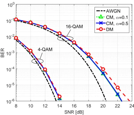
values already considered in the literature to be of practical interest [Ma-garini et al., 2011, Bisplinghoff et al., 2011]. The reader can consider that above those values, the transmission is so prohibitive that common constel-lation, e.g. QAMs, can not be considered. Hence, in these Subsections, one has to exploit strong codes and robust modulations [Pattan, 2000].

In the three Figures 2.8, 2.9 and 2.10 the results for the three values of

σPN ∈ S are reported. It is worth noting that, only σPN = 3· 10−2 and

σPN = 6.6· 10−2are below the threshold of σPN ≈ 0.1 rad that defines the

maximum standard deviation for which there is a good agreement between the two models. That threshold has already been observed in the previous Sections where dealing with the model properties, i.e. statistic of the phase noise, and mismatch power. In this Section that threshold is also validated through BER MC simulation.

(39)

SNR [dB] 8 10 12 14 16 18 20 BER 10-6 10-5 10-4 10-3 10-2 10-1 100 AWGN CM, α=0.1 CM, α=0.5 DM 16-QAM 4-QAM

Figure 2.8: BER versus SNR with QPSK and 16-QAM with σPN = 3· 10−2with QPSK

and 16-QAM.

Coherent demodulation of the discrete-time sequence is realized by pilot-aided trellis based demodulation scheme proposed in [Barletta et al., 2013]. Such a method is able to provide good tolerance to phase noise because it implements virtually optimal Bayesian tracking of the unknown phase. It relies on the insertion of known pilot symbols that are time-division multi-plexed with the information-bearing symbols. In the results shown in this Section a pilot overhead of 5% is used. Bayesian tracking [MacKay, 2003] is an important topic in this thesis and it will be introduced in Chapters 3 and 4.

Figure 2.8 reports the BER versus SNR for σPN = 3 · 10−2. An

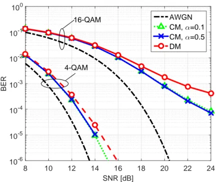
excel-lent fit is found between the BER curves of the two models. The AWGN performance is also reported as a reference in all Figures of this Section. In the case of σPN = 6.6· 10−2 the simulated BERs are shown in Figure

2.9. One can observe that for QPSK we still have a good agreement be-tween the two models, while, in contrast, with 16-QAM a small deviation appears at BER values lower than 10−3, being the performance achieved by DM slightly worse than that achieved by CM. Figure 2.10 shows results for σPN = 0.135. Due to strong phase noise, for both the two models a

(40)

SNR [dB] 8 10 12 14 16 18 20 22 24 BER 10-6 10-5 10-4 10-3 10-2 10-1 100 AWGN CM, α=0.1 CM, α=0.5 DM 4-QAM 16-QAM

Figure 2.9: BER versus SNR with QPSK and 16-QAM with σPN = 6.6· 10−2with QPSK

and 16-QAM.

BER floor is observed at high SNR with 16-QAM. The DM channel model exhibits a BER floor that is one order of magnitude lower than that of DM. From these results one concludes that when the DM channel model is used in computer simulations the resulting BER measure is always conservative. This gives to previous works exploiting DM rather than considering a CM approach an even more secure validation. Not only the DM is a good ap-proximation under the condition σPN < σPN, but it is even conservative in its

BER analysis. The true system can work even better because of the mem-ory introduced by all the filtering steps. Finally, in all the considered cases the roll-off factor has negligible impact on the BER performance achieved by the CM.

2.5

Phase Noise PSD

In this brief Section the author gives a frequency-domain analysis about the DM and CM mismatch, giving also a possible explanation of the better behavior of the CM compared to the DM.

(41)

SNR [dB] 8 10 12 14 16 18 20 22 24 BER 10-6 10-5 10-4 10-3 10-2 10-1 100 AWGN CM, α=0.1 CM, α=0.5 DM 4-QAM 16-QAM

Figure 2.10: BER versus SNR with QPSK and 16-QAM with σPN= 0.135 with QPSK and

16-QAM.

value of the its periodogram

|Px(f )|2 = T · E [ ∑N n=1xne j2πnf2 ] N , (2.23)

where T is the sampling time, i.e. symbol interval, and N the number of samples [Rabiner and Gold, 1975].

Recalling the simulation with block scheme as in Figure 2.2, the Power Spectral Density (PSD) of the two processes are simulated as the mean of the periodograms | ˆPx(f )|2 = T N M M ∑ m=1 N ∑ n=1 xnej2πnf 2 , (2.24)

where M is the number of averages of the periodogram taken by the simu-lator.

(42)

Normalized Frequency

10-6 10-5 10-4 10-3 10-2 10-1 100

Complex Exponential Periodogram [dB|

-100 -90 -80 -70 -60 -50 -40 -30 CM DM

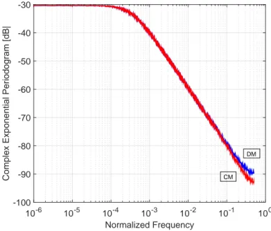
Figure 2.11: PSD of φiand φ′iof DM and CM respectively with σPN = 6.6· 10−2.

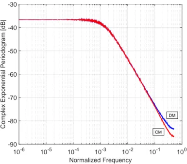
In Figures 2.11 and 2.12 the estimated PSDs of the DM and the CM phase noise complex exponential, i.e. ejφ and ejφ′, are plotted. In both scenar-ios, the CM phase noise PSD is narrower than the DM one. The difference between the two is apparent for normalized frequency greater than 10−1. This difference can be explained by observing that CM has been sampled after having been filtered through the matched filter, which increases the duration of the continuous-time phase noise memory thus narrowing the spectrum.

It is strongly intuitive that if one wants to track the phase noise in a carrier recovery system, the one with broader spectrum is worse tracked

[Rabiner and Gold, 1975]. The are several techniques to perform carrier recovery, like the Pilot-Aided trellis demodulation already presented [Barletta et al., 2013] or blind techniques, e.g. decision-directed-mode [Fatadin et al., 2009].

Finalizing the current dissertation, if one compares the results of this Sec-tion with the previous one about BER of the two models, he can find a sort of agreement in the behavior of the model mismatch. The better CM BER performances of the Bayesian tracking system in Section 2.4 find an explanation when comparing the two different PSD of the processes φ and

(43)

fre-Normalized Frequency

10-6 10-5 10-4 10-3 10-2 10-1 100

Complex Exponential Periodogram [dB|

-90 -80 -70 -60 -50 -40 -30 CM DM

Figure 2.12: PSD of φiand φ′iof DM and CM respectively with σPN = 0.135.

quencies can be better tracked by the low-pass nature of the Bayesian filter used to demodulate the sequence. This is another strong point to validate the results presented in the Chapter.

2.6

Conclusion

In this Chapter the limits of the symbol-spaced discrete-time channel model of Equations (1.1) that is commonly adopted to evaluate performance degra-dation introduced by discrete-time multiplicative Wiener phase noise have been analyzed. This so called Discrete Model (DM) is commonly assumed in the literature cited in this Chapter under the condition of “small” phase noise. However, nobody have yet studied how much “small” the phase noise must be.

Thus the author has derived the more accurate model obtained by filtering and sampling at symbol-rate the continuous-time received signal affected by multiplicative continuous-time Wiener phase noise reported in Equa-tion (2.9). In the Chapter this model is defined as Complete Model (CM). Particularly, CM takes into account the effects that affect a received signal before sampling and any Digital Signal Processing. The fit between the two models has been analyzed by means of statistical tests aiming to verify

(44)

temporal and distributional properties of both the DM and the CM phase noise processes. The power of the error resulting from the mismatch of the noiseless signals between the two models have also been simulated. One can conclude that, when the standard deviation of the discrete-time Wiener phase-noise increment is below the threshold of DM validity σPN = 0.1

rad, the discrete-time model provides a good approximation to the sampled filtered model with continuous-time phase noise with the same width of the spectral line. This can be concluded from the results of Section 2.3, where it is shown by MC simulation that the Power of the mismatch error is 20 dB below the power of the signals in the worst case, i.e. σPN → σPN. Note

that in most practical scenarios the values of σP N are way lower than the

threshold of validity of the DM.

The only notable difference between CM and DM phase noise process is the non-null correlation between the innovation of the phase noise ηi and itself

delayed by one sample. The little memory introduced however is negligible in practical application because the difference produced by exploiting this information has brought only a gain of 1 dB in terms of power of mismatch, that is already very low.

The good quality of the approximation is also demonstrated by analysis of Bit Error Rate performance, showing that BERs of QPSK and 16-QAM are close to each other for the two models. Moreover, from results coming from Sections 2.4 and 2.5, one can conclude that, not only DM is a good approximation of the CM when σPN < σPN, but the approximation is

con-servative. Indeed as one can see from Sections 2.4 and 2.5 DM’s BER is always a little bit worse than the CM one and the DM phase noise process is a bit more difficult to track with a carrier recovery system for its higher PSD components with high normalized frequencies.

(45)

CHAPTER

3

Bayesian Inference in State-based

Problems

Bayesian inference is the process of fitting a probability model to a set of data and summarizing the result by a probability distribution on the param-eters of the model and on unobserved quantities such as prediction for new observation.

After an introductory Section about Bayesian Inference, the author focuses the attention on the tracking of unknown processes, e.g. phase noise, to better analyze Channel performances and its models [Gelman et al., 2014]. Bayesian tracking is a really powerful tool, but it has its own limits when experiencing complex state models, e.g. physical transmission over an op-tic dispersive channel. This last one will be used as an example of the limits of such approach in the last Chapter Section.

3.1

Bayesian Tracking of Channel State

As it is said in the Introduction, Bayesian Tracking can be exploited in many applications. The main objective of a communication system is the transfer of information over a channel [Nguyen and Shwedyk, 2009]. When

Analysis of Wiener phase noise issues in optical transmission systems

A

NALYSIS OF

W

IENER

P

HASE

N

OISE

I

SSUES IN

O

PTICAL

T

RANSMISSION

S

YSTEMS

Abstract

I

Contents

List of Figures

List of Tables

List of Acronyms

CHAPTER

1

Introduction

1.1

1.2

1.3

CHAPTER

2

Modeling the phase Noise

2.1

h(t)

a

w(t)

e

h(-t)

r(t)

y(t)

y

2.2

10

10

0

0.1

0.2

0.3

σ

PN

PPC

1

16−QAM

α

= 0.1

16−QAM

α

= 0.5

QPSK

α

= 0.1

QPSK

α

= 0.5

10

10

0

0.1

0.2

0.3

σ

PN

PPC

2

16−QAM

α

= 0.1

16−QAM

α

= 0.5

_e

_PN

_PN

_PN