Scuola di Dottorato in Ingegneria “Leonardo da Vinci”
Corso di Dottorato di Ricerca in Ingegneria Meccanica
Elastohydrodynamic lubricated contacts under transient conditions
Tesi svolta per il conseguimento del titolo di dottore di ricerca
Candidato
Ing. Kenred Stadler
Tutori
Prof. Ing. Enrico Ciulli (DIMNP, Pisa)
Prof. Ing. Bruno Piccigallo (Accademia Navale, Livorno)
VI Ciclo 2008
Abstract
Many Elastohydrodynamic lubricated (EHL) contacts, such as rolling element bearings, gears or cam systems work under transient conditions due to changes in speed, load, or geometry. A better tribological understanding is necessary in order to give further insights and guidelines to engineers who need to design systems with EHL contacts experiencing transient conditions. However, due to the complexity a lot of fundamental research done in the field of EHL is mostly concentrated on steady-state conditions.
In this work, experimental investigations with an interferometric test rig as well as numerical studies have been carried out. At the University of Pisa, the existing experimental setup was modified in order to test under transient conditions. This involves also the development of new tools in order to analyze efficiently the results such as the film thicknesses and friction coefficients. For example, an image-processing tool was developed in order to reconstruct out of a white light interferogram the deformed surface of an EHL contact.
In particular the influence of thermal effects combined with transient effects was investigated. Thermal effects are caused by high slide-to-roll ratios, or contacting materials with different properties, whereas transient effects by changing the velocity over time. If the contacting materials have different thermal properties, at some contact conditions non-standard film shapes different from the usual EHL shape with a so-called “dimple” in the center of the contact exist. This can have some influence on the film thickness and hydrodynamic friction coefficient under steady state as well as transient conditions.
In collaboration with the University of Kyushu in Japan, as a study object for a numerical investigation a reciprocating EHL rolling point contact was chosen. In this field few studies exist and are of interest because the lubrication state of oscillating machine elements is often influenced by cavitation phenomena. Due to the complexity caused by the non-steady state and cavitation phenomena, there is no design equation for the oil-film thickness under oscillatory motion, while reliable estimations can be done for steady state conditions. Based on recent numerical solution methods a Multilevel Multigrid (MLMG) algorithm was developed in C/C++, which made it possible to carry out parametric studies relatively fast. With the help of the algorithm, as an intermediate step to obtain a future design equation, a first equation to predict the length of cavity at the outlet of an EHL contact has been developed. The knowledge of the cavity length is of importance, because after reversal of the rolling direction the outlet region becomes the new inlet region and thus the cavitation produced beforehand can be entrained into the conjunction. This can lead to starvation effects, which in turn can cause a decrease in film thickness and increase in wear. In addition, first complete simulations of reciprocating EHL rolling point contacts have been carried out and shown good agreement when comparing with experiments.
Sommario
Molti contatti in regime elastoidrodinamico (EHL), quali ad esempio quelli nei cuscinetti a corpi volventi, nelle route dentate, o nei sistemi con camme, lavorano in condizioni transitorie dovute a variazioni di velocità, carico o geometria. Nonostante ciò, data la complessità dell’argomento, molte ricerche effettuate nel campo dell’EHL si sono concentrate in passato su condizioni stazionarie. Una più approfondita conoscenza tribologica è però oggi necessaria per poter fornire più dettagliate informazioni ai progettisti.
L’attività svolta ha riguardato sia ricerche sperimentali sia studi numerici.
Per l’attività sperimentale è stata utilizzata un’attrezzatura interferometrica che è stata opportunamente modificata in modo da effettuare le prove EHL in condizioni di transitorio. Nuovi software sono stati sviluppati sia per la gestione delle prove sia per un’analisi più adeguata dei risultati, riguardanti il coefficiente d’attrito e l’altezza del meato (ad esempio è stato realizzato un software capace di ricostruire la deformata di un contatto EHL partendo da un interferogramma in luce bianca). È stata in particolare studiata l’influenza degli effetti termici, causati dagli alti valori di strisciamento o dalle diverse proprietà dei materiali a contatto, combinati con quelli dei transitori ottenuti con variazioni della velocità in funzione del tempo. Se i materiali di contatto hanno diverse proprietà termiche, in determinate condizioni di prova il meato assume forme diverse da quella classica, in particolare con l’insorgere del cosiddetto “dimple” nel centro del contatto. Ciò può avere una qualche influenza sulle altezze del meato e sul coefficiente d’attrito sia in condizione stazionarie, sia in condizioni transitorie. L’attività di tipo numerico ha riguardato prevalentemente lo studio di un contatto EHL di punto in moto alterno. In questo campo esistono ancora pochi studi anche perché sono spesso presenti fenomeni di cavitazione che rendono difficile l’indagine. A causa della complessità dovuta alla condizione transitoria ed ai fenomeni di cavitazione non esiste ad esempio un’equazione di progettazione per la stima dell’altezza del meato in condizioni oscillatorie, mentre si possono avere stime affidabili per i casi stazionari. È stato sviluppato un algoritmo
multilevel multigrid (MLMG) in C/C++ che ha consentito di eseguire studi
parametrici in tempi relativamente brevi. È stata quindi ricavata un’equazione per la stima dell’ampiezza della zona cavitata all’uscita del contatto EHL, quale primo passo per ottenere in futuro una formula di pratica utilità per la progettazione. La conoscenza dell’ampiezza della zona cavitata è particolarmente importante poiché dopo l’inversione del moto tale zona si trova all’ingresso del contatto con possibili effetti di mancanza di lubrificante, e quindi di riduzione di altezza del meato e aumento d’usura. Con il programma realizzato sono inoltre possibili simulazioni numeriche complete di un contatto EHL in condizioni di moto alterno.
Contents
Chapter 1 Introduction ...1
1.1 Elastohydrodynamic lubrication ...1
1.1.1 General aspects...1
1.1.2 Pressure profile and film shape of EHL contacts ...2
1.2 Research in the field of EHL – a historical review ...7
1.3 Background and objective of this thesis ...9
1.4 The layout of this thesis ...13
Chapter 2 Experimental procedure for transient conditions ...17
2.1 Experimental apparatus of the DIMNP ...17
2.2 General experimental procedure ...20
2.2.1 Data acquisition ...22
2.2.2 Camera trigger...23
2.2.3 High speed camera...25
2.3 Analysis of the friction coefficients under transient conditions ...28
Chapter 3 Measurement of the film thicknesses ...34
3.1 Existing solution at the DIMNP ...34
3.2 Optical interferometry – basic principals...36
3.2.1 Monochromatic light...37
3.2.2 White light ...39
3.2.3 Trichromatic light ...40
3.3 White light image processing ...41
3.3.1 Basic principle...42
3.3.1.1 Differential colorimetry ...42
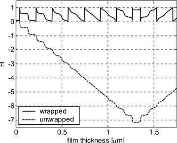
3.3.1.2 Phase unwrapping ...43
3.3.2 Concept of the image processing software ...50
3.3.3 Calibration table...51
3.3.4 Consideration on accuracy ...55
3.3.5 Example of white light program use ...57
3.3.6 Concluding remarks...61
3.4 Monochromatic light image processing ...63
3.4.1 Example of monochromatic light program use ...63
4.1 Experimental conditions ... 72
4.2 Film thickness investigations... 74
4.2.1 Film thickness results under steady state conditions ... 74
4.2.2 Film thickness results under transient conditions ... 79
4.3 Friction coefficient results... 83
4.3.1 Friction coefficient results under steady state conditions ... 84
4.3.2 Friction coefficient results under transient conditions... 89
4.4 Discussion ... 93
4.4.1 Film thicknesses ... 93
4.4.2 Friction coefficients ... 95
4.4.2.1 Influence of temperature viscosity wedge action on friction 95 4.4.2.2 Influence of the test rig characteristics on friction ... 97
4.4.3 Friction coefficient – Film thickness relation ... 98
4.4.4 Steady state friction coefficient measurements ... 99
4.5 Conclusions and considerations ... 100
Chapter 5 Numerical investigations ... 105
5.1 Numerical methods in the field of EHL... 105
5.2 Governing equations for the study of EHL ... 108
5.2.1 The Reynolds Equation... 108
5.2.2 The film thickness or deformation equation ... 109
5.2.3 The force balance equation ... 110
5.2.4 The lubricant model ... 110
5.2.4.1 Density equation... 110
5.2.4.2 Viscosity equation ... 111
5.2.5 Dimensionless equations ... 111
5.2.6 Dimensionless parameters ... 114
5.2.7 Discrete equations ... 116
5.3 Multilevel Multi-Grid method... 119
5.3.1 Correction Scheme (CS)... 120
5.3.2 Full Approximation Scheme (FAS) ... 122
5.3.3 Coarse grid correction cycle ... 123
5.3.4 Full Multigrid (FMG) ... 124
Chapter 6 Solving transient EHL problems ...135
6.1 Implementation of the transient term ...135
6.1.1 Verification and comparison for a transverse ridge ...142
6.1.2 Verification and comparison for a traversing cavity...144
6.2 Reversal of entrainment...146
6.2.1 Example of entrainment velocity reversal...147
6.3 Implementation of starvation effects ...148
6.3.1 The Elrod algorithm ...149
Chapter 7 Investigation of reciprocating EHL rolling point contacts...156
7.1 Cavitation in EHL contacts...157
7.1.1 Measurement of cavity pressure ...159
7.2 Simulation of the cavitation region...160
7.2.1 Output of the program ...162
7.3 Parametric study and equation for cavity length...165
7.3.1 Dependency of cavity length on Moes parameters ...166
7.3.2 Correction factors for cavity length equation ...170
7.3.3 Equation to estimate cavity length...172
7.4 Experimental verification of cavity length equation...174
7.4.1 Experimental setup and procedure...174
7.4.2 Results and discussion...176
7.5 Simulation of a reciprocating EHL rolling point contact ...181
7.5.1 Set of simulation parameters...181
7.5.2 Results and discussion...182
7.6 Conclusions...186
Chapter 8 Summary and perspective...189
References ...193
Appendix A System of equations...199
Notation
a half width of Hertzian contact
A amplitude of cavity or ridge, or matrix of coefficients ca light attenuation coefficient
D diameter of steel ball
eh,H discretization error on fine grid or coarse grid E’ reduced modulus of elasticity
f friction coefficient or test frequency
fh,H right hand side vector on fine grid or coarse grid
F applied load
G Hamrock and Dowson dimensionless material parameter Gh finest grid level (G2h next coarser level, etc.)
h dimensional film thickness hcen central dimensional film thickness hmin minimum dimensional film thickness
h mesh size
h00 dimensional central offset film thickness (rigid body approach) H dimensionless film thickness
H00 dimensionless central offset film thickness (rigid body approach) HSV hue, saturation, value color space
Hu hue component of an HSV image (phase unwrapped) Hw hue component of an HSV image (phase wrapped) Hcen central dimensionless film thickness
Hcff central fully flooded dimensionless film thickness Hinlet dimensionless height of lubricant at inlet
Hoil dimensionless height of lubricant at inlet i, j, k, t integer indices (nodes on calculation domain)
I, J coarse mesh integer indices (nodes on calculation domain) I0, I1, I2 light irradiances h H I interpolation operator H h I restriction operator K film thickness kernel matrix
thermal loading parameter
m, m1, m2 multilevel multi-integration correction patch widths M Moes dimensionless load parameter
n rpm or refractive index of lubricant nx,y number of mesh points
N total number of mesh points in computational domain
p dimensional pressure
p0 pressure coefficient in Roelands equation pcav dimensional cavitation pressure
pHz maximum Hertzian pressure pvacuum vacuum pressure (-0.1013 MPa)
P dimensionless pressure
Pcav dimensionless cavitation pressure rh,H residuum on fine grid or coarse grid
R, Rx, Ry reduced radii of curvature in X and Y directions
R radius of cavity
Rq mean square roughness
RGB red, green, blue color space S slide-to-roll ratio
t dimensional time
T dimensionless time or temperature uh,H general solution on fine grid or coarse grid
u1, u2 velocities of contacts 1 and 2 respectively, in the X direction ud circumferential speed of the glass disc
us circumferential speed of the steel ball sum of velocities of contacts
um average velocity of contacts
U Hamrock and Dowson dimensionless speed parameter W Hamrock and Dowson dimensionless loading parameter
applied load
wavelength of ridge
x, y dimensional coordinates X, Y dimensionless coordinates
Xc dimensional cavity length
Xd dimensionless position of surface defect z viscosity index (Roelands equation)
α pressure viscosity index (piezoviscosity index) α sim reference value (parametric study, 26.3 GPa-1) β temperature viscosity coefficient
δ change applied after relaxation ΔT non-dimensionalised timestep size
ΔX, ΔY mesh sizes in X and Y directions respectively ε coefficient in dimensionless Reynolds equation η0 viscosity at ambient pressure
η dimensional viscosity
η dimensionless viscosity θ fractional film content κ thermal conductivity
λ coefficient in dimensionless Reynolds equation
light wave length
Λ lambda ratio (dimensionless film thickness parameter) ν0 number of coarse grid smoothing cycles
ν1 number of pre-smoothing cycles ν2 number of post-smoothing cycles ρ0 density at ambient pressure
ρ dimensional density
ρ dimensionless density φ angle in polar coordinates
Φ phase shift
ω underrelaxation factor
Ω solution domain
CHAPTER 1
INTRODUCTION
Tribology can be described as a study that deals with the design, friction, wear and lubrication of interacting surfaces in relative motion. In engineering this field of study is still underestimated even if tribological problems in industrialized countries cause economical losses in the range of billions Euro/year [32]. The field of tribology includes problems in nearly all technical fields, from the aerospace industry like a “high-tech" bearing used in a spacecraft to medical problems in bioengineering like an artificial joint. The understanding of the underlying mechanisms requires an interdisciplinary knowledge from fields, such as physics, chemistry, materials science, mechanical engineering and mathematics.
In this thesis an important tribological phenomenon is studied: Elastohydro-dynamic lubrication.
1.1 Elastohydrodynamic lubrication
1.1.1 General aspectsElastohydrodynamic lubrication, hereinafter referred to as EHL, is a relatively recent branch of tribology which only became properly established in the early nineteen sixties. The topic is concerned with understanding and modeling lubrication problems in which solid surfaces deform under large pressures. In EHL contacts two solids are pressed against each other and the lubricant, present in the gap between the solids, prevents the two surfaces from touching. The contact pressures are so large that the elastic deformation of the solids is of the order of the lubricant film thickness (even higher). EHL contacts are present in many non-conformal mechanical systems, e.g. gears, cams and rolling element bearings as shown in Figure 1-1.
Figure 1-1: Typical EHL contacts (source: [13]).
At high contact pressures, up to 3.0 GPa, the viscosity will increase rapidly (piezoviscosity). This will change the behavior of the lubricant and strongly affect the fluid film formation. Therefore the viscosity-pressure relation and, in more general terms, the lubricant rheology is an essential element in the study of EHL. EHL is not only restricted to the aforementioned highly loaded contacts between steel surfaces; often called Hard-EHL. It applies also to situations where the stiffness of one or both solids in contact is small compared to the pressure in the lubricant film; often called Soft-EHL. Typical examples are rubber sealing’s, elastically distorted journal bearings or hip joint spherical pairs.
1.1.2 Pressure profile and film shape of EHL contacts
A typical EHL contact is illustrated in Figure 1-2. The entrainment of the lubricant is from the right to the left. In the inlet region the pressure starts to increase smoothly. Closer to the contact center the pressure slope decreases rapidly until the maximum pressure is reached (often close to the Hertzian pressure). Then the pressure decreases rapidly apart to a small region in the outlet area. There, a typical EHL feature develops; a pressure spike [72] followed by a local constriction in the film thickness (this pressure peak can reach values higher than the maximum Hertzian pressure). At the end of the contact region the pressure solution is zero (ambient pressure) in what is known as the cavitation region. This means that the lubricant film is no longer continuous; bubbles of air at ambient pressure are present in the oil film.
Figure 1-2: Pressure profile and film thickness of a typical EHL contact (source: [http://www.ime.rwth-aachen.de,2003]).
For most kinematic conditions in EHL the film thickness or deformation remains constant in the contact area (often referred to as central film thickness). The constriction in the outlet region contains the minimum film thickness. As a fast explanation, in high load cases such as EHL, the oil-film boundaries will diverge comparatively rapidly beyond the thin film zone. In the outlet region the pressure drops very fast to the ambient pressure, thus the pressure curve must terminate very near to the end of this zone. Consequently, in this zone large pressure gradients must exist to reduce the pressure to ambient pressure. Large pressure gradients at low pressures and low viscosities can be achieved only by a reduction in the film thickness. Thus, as shown in Figure 1-2, a local reduction in the film thickness occurs near the end of the thin film zone.
As already mentioned, compared to the classical hydrodynamic pressure buildup, in EHL two additional effects are present. Figure 1-3 illustrates the elastic deformation and the piezoviscosity. When the surfaces approach, the lubricant fluid pressure significantly increases. This leads to an increase of the viscosity with pressure (piezoviscosity) and the elastic deformation of the
surfaces in contact (this depends also on the contacting materials and lubricant used). The elastic deformation (h1 in Figure 1-3) as well as the piezoviscosity effect (h2 in Figure 1-3) leads to a significant increase of the film thickness. The film thickness predicted by the classical hydrodynamic theory would be significantly lower.
Figure 1-3: Effect of the elastic deformation and viscosity on EHL film generation (source: [http://www.ime.rwth-aachen.de,2003]).
Following, the most important parameters which influence the film formation in an EHL contact will be briefly introduced. Similar to the hydrodynamic lubrication theory, also in EHL contacts the film thickness depends on the hydrodynamic velocity (summation of the surface velocities in contact) and the load. With increasing velocity and decreasing load the film thickness increases and vice versa decreases with decreasing velocity and increasing load. For low velocities (or very high loads), the elastic deformations of the contacting bodies dominate. In this case the pressure distribution in contact will be very similar to the static Hertzian pressure distribution as can be seen in Figure 1-4. Furthermore for higher velocities the pressure distribution changes from the typical EHL case to the rigid body case [26]. In Figure 1-5 it can be seen that with increasing load the maximum pressures moves to the center of the contact and resembles the Hertzian pressure distribution.
Figure 1-4: Influence of the hydrodynamic velocity on EHL pressure distribution (1-lowest speed, 5-highest speed) (source: [26]).
Figure 1-5: Influence of the load on EHL pressure distribution (source: [http://www.ime.rwth-aachen.de,2003]).
An important parameter besides the velocity and the load is the viscosity, or more in general the lubricant itself. The viscosity and piezoviscosity (often also referred to as pressure viscosity index) influence the pressure distribution and also to what extend the pressure spike in the outlet region will develop. As an example, in Figure 1-6 the pressure distribution for two different oils is shown.
Figure 1-6: Influence of the oil property on EHL pressure distribution (source: [http://www.ime.rwth-aachen.de,2003]).
Figure 1-7: Influence of geometry on EHL pressure distribution (top: point contact, bottom: line contact) (source: [http://www.ime.rwth-aachen.de,2003]).
Naturally the geometry has also a big influence on the EHL film thickness and pressure distribution. In most cases one distinguishes between point contacts (e.g. ball-on-disc) and line contacts (e.g. cylinder-on-cylinder). In Figure 1-7, the pressure distribution of an EHL point and line contact is shown. (In line contacts often two infinite long cylinders are assumed, or that border effects are negligible.) In a point contact the pressure distribution changes in entrainment direction and transversal to the entrainment, whereas in line contacts only in the
direction of entrainment. In addition, line contacts support usually higher loads (depending on the axial contact length).
In the next section, a short summary of important works in the field of EHL is given. To summarize the complete work by many outstanding researchers in a few pages is somewhat difficult. In the literature there are comprehensive reviews for example Dowson and Ehret [24].
1.2 Research in the field of EHL – a historical review
The theory of lubrication was more or less born during the end of the 19th century. Stimulated from the experimental investigation of friction in lubricated journal bearings by Tower [87] where substantial pressures in the oil film have been accidentally discovered, Reynolds [75] derived the basic differential equation of fluid film lubrication, nowadays well known as “Reynolds Equation”. The equation relates the pressure in the lubricant film to its geometry and the velocity of the moving surfaces. He compared his theoretical results with the experiments of Tower. Reynolds’ equation was the first mathematical tool for the design of bearings. At approximately the same time, Hertz [45] was the first to describe the elastic deformation of two, non-conforming solids in contact and Barus [7] developed an exponential viscosity-pressure relation. It took about further 50 to 60 years until these pioneering works have been combined into what is now known as Elastohydrodynamic lubrication theory, EHL.
Successful application of Reynolds’ theory in the beginning of the 20th century to journal and thrust bearings failed when trying to model lubrication in gears. Martin [63] considered an isoviscous lubricant between two smooth rigid cylinders, representing the gear teeth. A relationship between the operating conditions and the minimum lubricant film thickness was obtained. However, the film thicknesses predicted were significantly less than the known surface roughness of gears. It was concluded that the successful operation of gears almost without wear as observed in practice could not be ascribed only to the fluid film action.
Almost 30 years after Martin the contradiction between theory and practical observations was solved first by Ertel [29] and Grubin [34]. They included the elastic deformation of a dry contact due to the high contact pressures and the
increase in viscosity with increasing pressure in the theoretical analyses. From the solution of Reynolds’ equation in the inlet region, with the elastic deformations according to Hertz [45] and the linear relation between the logarithm of the viscosity and the pressure proposed by Barus [7] a first film thickness estimation equation for the center of a line contact was derived. Compared to previous works the predicted film thicknesses were larger than the roughness of gears. The work of Ertel and Grubin provided the basis for the EHL theory. Since then, considerable progress has been made. Experimental techniques in order to evaluate the film thickness and pressure distribution as well as sophisticated numerical algorithms for the solution of the basic governing equations have been developed.
A first complete numerical solution of an EHL line contact was obtained in the beginning of the fifties by Petrusevich [72]. With the low computing power available at this time and the added mathematical difficulties a two dimensional point contact was impossible to solve. With the further development of computational power in the seventies Hamrock and Dowson [43] presented numerical solutions for a two dimensional EHL contact for a wide range of parameters involved. They combined these solutions to the first film thickness formula for point contacts. But the research was not limited to numerical studies. In parallel researcher like Roelands [76] developed a new lubrication model with a correlation between pressure, viscosity and temperature. His lubrication model is still in use nowadays.
Starting from the eighties computers became really powerful and numerical algorithms more and more efficient. Different approaches to solve the governing equation contemporary as direct methods by means of Gauss-Seidel iterations or by Newton-Raphson algorithms’ [70] or by indirect methods [30] have been developed.
Brandt [4] introduced the powerful multigrid method which has been applied to EHL lubrication by Lubrecht [59]. At the beginning of the nineties, Venner [89] could improve the multigrid approach. He resolved the convergence problem for high loads by distributive line relaxation. This allowed Lubrecht & Venner and many other researchers the study of more realistic EHL contacts conditions. Surface roughness and several transient conditions, by means of changing load,
velocity, geometry or all combined together have been simulated. The numerical works of Chang [11], Ai [1] and Hooke [48] dealing with line as well as point contacts are some examples. The influence of thermal effects can also be simulated by adding to the Reynolds and elastic deformation equation the energy equation, e.g. [86].
Reviewed so far briefly research activities with respect to the development of numerical algorithms, it needs to be mentioned that, also experimental techniques had been considerably improved. Given that a great part of this work is focused on experimental investigation, a very important experimental technique, applied also in this work, was basically developed by Gohar & Cameron [35] and Foord [31]. They introduced the optical interferometry method to EHL lubrication in order to measure the film thickness. Compared to capacitive techniques this method allows a very detailed measurement of the EHL contact shape and the film thicknesses up to the nanometer scale. In contrast, capacitive methods allow mostly only the measurement of an average film thickness and pressure.
The optical interferometry method was significantly refined by many researchers like Cann [10], Johnston [54], Sugimura [82] and Marklund [60]. Thus, it was possible to verify numerical simulations by experimental observations and to find new phenomena as for example done by Kaneta [55]. Experimental findings in turn should be included and explained also by numerical simulations. Since a numerical simulation is only as good as the theoretical model assumed, experiments can never be replaced by simulations to hundred percent. An appropriate combination of both, theoretical as well as experimental work is often necessary.
Also this work is describing experimental as well as numerical investigations. Some direct comparison with numerical and experimental results is done for the study of a reciprocating EHL rolling point contact presented at the end of this thesis.
1.3 Background and objective of this thesis
The tribology group at the University of Pisa has worked many years in the field of EHL lubrication. The research on EHL includes investigations for real
applications as well as fundamental studies. For example, in cooperation with the Avio® Aerospace Group the tribological behavior of gears is studied using high performance test rigs, whereas fundamental studies are carried out by using simple model geometries such as ball-on-disc machines.
The work presented here focus mostly on fundamental studies in the field of EHL. In Pisa, at the Department of Mechanical, Nuclear and Production Engineering (subsequently referred to as DIMNP) experimental investigations have been carried out with a closer look on thermal effects and transient effects. Some of these studies are reported for example in Bassani [2] and Ciulli [21]. This relatively fundamental study is of interest, because many machine elements such as roller bearings, gears and cams work under conditions where the effect of sliding is not negligible anymore. Even more the usage of non-metal materials like ceramics becomes more and more attractive in industry in order to reduce weight, to have a higher stiffness or because of the thermal resistance. However, different thermal properties of the contacting surfaces may influence the film formation and friction [23].
For pure rolling conditions (no sliding), works of e.g. Grubin [34], Dowson and Higginson [26] brought fundamental understanding of the working performance of machine elements with non-conformal lubricated contacts, by developing the EHL theory. Several studies have been made taking into account sliding effects. Wilson [96] and Olver [71] developed formulas where the deviation from the pure rolling film thickness values can be calculated by a correction factor and explained by inlet heating, or a temperature rise can be calculated by the bulk and flash temperature theory [52]. Smeeth and Spikes [79] tried to explain some of their experimental findings, measurements of the film thickness for different slide-to-roll-ratios S under steady state conditions, with the theory explained in [71],[96]. However, the inlet heating and rise in bulk temperature could explain the change in film thickness by different S only to some extent. Further insights were gained with the experimental work of Cameron [9] and Kaneta [55]. Kaneta has shown the formation of a dimple in the central part of the contact under high sliding conditions if materials with different thermal properties are used. The classical theory, however, assumed a flat plateau in the central part of the contact and the film thickness and shape are mainly determined by the
conditions at the entrance to the contact. In [56], Kaneta and Yang could verify the experimental findings with numerical simulations by solving also the energy equation and explaining the occurrence of dimples with the so-called temperature viscosity wedge effect.
So far most of these works were using steady state condition in order to explain thermal effects caused in sliding contacts. But it must be considered that most of the machine elements are working under transient conditions by means of changing radius of curvature, load or speed. In some experimental and numerical works using transient conditions, such as the ones of Sugimura [83] or Zhao [102], the effect of squeeze on the film thickness was investigated. In Zhai [101] friction coefficients have been simulated under transient conditions for a mixed contact. The effects of different slide-to-roll ratios combined with a change in velocity, however, are rarely investigated. First investigation have been done by Ciulli [17], who analyzed EHL friction coefficient data under transient conditions combined with sliding.
In this thesis, experimental studies such as [17] and [20] have been continued by modifying the existing experimental setup at the DIMNP. The experimental procedure such as the data analysis was improved in order to carry out efficiently EHL tests under transient conditions. In particular, friction coefficients and film thicknesses obtained when combining both, transient effects and thermal effects have been investigated. The research, however, consisted not only of experimental but also of theoretical components, as this adds more reality to the research project. A robust algorithm capable of simulating transient EHL point contacts was developed and applied to reciprocating EHL rolling point contacts. The final part of the numerical investigation has been carried out at the Kyushu University (Japan) in the Department of Mechanical Engineering Science (subsequently referred to as DMES).
In the field of reciprocating EHL contacts few studies exist and are still of interest because the lubrication state of oscillating machine elements is often influenced by cavitation phenomena. After reversal of the rolling direction the outlet region becomes the new inlet region and thus the cavitation produced beforehand in the outlet region can be entrained into the conjunction. The knowledge of the
lubrication state of such EHL contacts working under non-steady state conditions is very important in order to prevent wear or even complete failure. There are some works with respect to EHL contacts under non-steady state conditions, which try to contribute with relatively easy to use expressions or formulae for practical use. Hooke [47] has analyzed film thickness during reversal of entrainment in EHL line contacts and derived film thickness formulae. Sugimura et al. [84] developed an expression for EHL point contacts to estimate the film thickness under acceleration or deceleration and compared some of the results with Hooke. Unfortunately the use is still hindered, because a constant for the upstream distance must be estimated by experience or by experimental observations. Messe et al. [64] derived a method for a line contact to calculate the part of the film thicknesses were the Couette flow dominates. Close to the boundaries, however, where the pressure falls to zero and the minimum film thickness develops the Poiseuille flow becomes important. All those studies show that, EHL under transient conditions still needs further research. In addition, these works are assuming fully flooded conditions but these conditions are unfortunately not always found in real applications.
Wedevsen et al. [93] studied starvation phenomena for different supply conditions by optical interferometry. An important observation was that an oil-air meniscus is formed in the inlet region and moves towards the Hertzian contact circle as starvation increases. He developed formulae in order to predict film thickness based upon the position of the oil inlet meniscus. In numerical studies Hamrock and Dowson [44] adopted the inlet meniscus position method to describe starvation. The studies above are limited because in real applications the position and form of the oil inlet meniscus cannot be measured or estimated. Elrod [28] proposed an algorithm that automatically determines the position and shape of the meniscus between starved and pressurized regions. Chiu [12] studied starvation but also the amount of oil left in the track in a rolling contact system. He developed analytically a first replenishment model based on surface tension. Furthermore he derived expressions to estimate the film thickness based on the amount of oil replenished. Wikstroem et al. [95] stated that the time for replenishment only by surface forces in a rolling bearing is too short. Probably many effects, such as surface tension, spin, vibration and oil drops
refeed depending on the working conditions play an important role. Further research is still necessary.
In the experimental work of Nishikawa et al. [68] a significant reduction in film thickness due to starvation in a reciprocating point contact was shown depending on the stroke length. Izumi et al. [49] simulated a reciprocating rolling point contact for fully flooded and starved conditions. The influence of cavitation effects in his numerical model was too severe since no replenishment was included. Wang [92] and Kaneta et. al. [57] simulated pure rolling EHL of short stroke reciprocating motion and compared the results with experiments. Observations were done for two test frequencies. They implemented the replenishment of oil into the numerical model based on the experimental observation of the oil film layer at the meniscus position. Good agreements between numerical and experimental results were found. The practical usage, however, is probably limited to the few experimental conditions observed. Nevertheless, the numerical investigations done are very useful as a tool for further developments of easy to use expressions in engineering applications. Recently, Sugimura [85] and Izumi et al. [50],[51] introduced in their numerical analysis a cavity pressure and found good correspondence in cavity shape and size with experimental observations. The present work adopted this definition of cavity pressure for reciprocating EHL rolling point contacts.
The aim of the numerical investigation was not only to simulate a reciprocating EHL rolling point contact including the effect of cavitations but also the development of a first equation for the cavity length. This equation is easy to use and may give additional insights into the lubrication state of an oscillating EHL point contact together with film thickness estimations by other researchers, as reported before.
1.4 The layout of this thesis
Due to the organization of the work described above, this thesis can be divided into two parts. The following four chapters will focus on studies with the existing test rig of the Pisa tribology group. So far experimental EHL investigations at Pisa have been basically carried out under steady state conditions. In order to investigate also under transient conditions, by means of changing speeds, some
modifications were necessary. For example, as explained in Chapter 2, existing LabView® control programs had to be modified and extended. The experimental apparatus uses optical interferometry for film thickness measurements. Under transient conditions a high speed camera is needed in order to record fast events. The correct use of a high speed camera is tricky and therefore some important considerations will be given. In addition, the way of analyzing experimental results such as the traction coefficients and the film thicknesses is compared to tests carried out under steady state conditions different and new methods must be found. As written in Chapter 3, the film thickness and shape analysis has been significantly improved and speeded up by automatic image processing. A Matlab® program using recent image processing methods is developed. In Chapter 4, experimental observations combining thermal and transient effects by running tests for different slide-to-roll ratios and changing the speed over time with a sinusoidal law are reported. Due to the complexity of several effects interacting together such as transient squeeze effects and thermal effects like inlet heating or the temperature viscosity wedge action, it is still very difficult to interpret the results completely. That is why similar experiments are rarely found in literature. The basic findings will be presented and discussed.
The second half of this thesis will concentrate on numerical investigations. An accurate prediction of the film thickness and pressure in EHL contacts working under practical relevant situations is important. A common situation in engineering is reciprocating motion. This requires an algorithm that allows solutions with a large number of nodes (very fine grid) in a reasonable computing time. Therefore, it has been decided to start the numerical investigation using a recent multi level multi grid (MLMG) program which was developed by Lubrecht and Venner [91]. The starting program calculates the film thickness and shape as well as the pressure distributions for a steady state EHL point contact.
In Chapter 5, after a short theoretical introduction of the governing equations and the necessary mathematics needed for understanding the basic idea of the algorithm, further developments of the program will be presented and discussed in Chapter 6.
The goal was the development of a program which can simulate a reciprocating EHL rolling point contact including starvation effects due to cavitations. Thus the previous program has been extended step by step. First the program was extended to transient conditions by including the squeeze term into the Reynolds equation. In order to check the intermediate program versions, test simulations by introducing model roughness have been compared with results found in literature. Next, reciprocating motion was implemented, and again some results have been compared with other works. Following, starvation effects were introduced by implementing the well-known Elrod algorithm. In Chapter 7, after modifications by some assumptions, the cavitation region as observed in reciprocating EHL rolling point contacts could be simulated. This new numerical tool made a parametric study possible in order to find expressions easy to use for practical applications. An equation that estimates the cavity length at the outlet of an EHL point contact could be derived and was compared with experimental observations. At the end of Chapter 7, some complete transient simulations have been also compared with experiments.
CHAPTER 2
EXPERIMENTAL PROCEDURE FOR TRANSIENT CONDITIONS
2.1 Experimental apparatus of the DIMNP
The tribology laboratory of the DIMNP at the University of Pisa is furnished with a test rig for lubricated contacts as can be seen in Figure 2-1. All the investigations in Pisa have been done with this apparatus. The current situation of the test rig is reported in the following.
DC motor (1) high speed camera stereo microscope xenon lamp shaft for specimen gas bearing oil supply
shaft for disc
oil refeed DC motor (2) DC motor (1) high speed camera stereo microscope xenon lamp shaft for specimen gas bearing oil supply
shaft for disc
oil refeed
DC motor (2)
Figure 2-1: Test rig for lubricated contacts at the DIMNP.
Pure rolling conditions and combined rolling and sliding can be simulated. The test rig allows friction force measurements, but is also equipped for optical interferometry and digital image acquisition with a high speed camera. Furthermore, the test rig allows also the use of different geometries. A ball on
disc as well as a cylinder on disc contact for different radius of curvatures can be tested. The apparatus, however, is not limited only to non-conformal contacts. With little modifications by fixing the rotating shaft it is also possible to test for thrust bearing pads or for other defined model geometries.
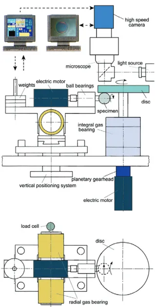
Figure 2-2: Schematic side view (top) and top view (bottom) of the major components of the test rig.
A schematic representation of the test apparatus is given in Figure 2-2. In order to test different slide-to-roll ratios, the specimen and the disc are driven by two separate DC motors. The slide-to-roll ratio S is defined to be:
s d e u u S u − = ( 2-1 )
and ue is the entraining velocity defined as
2
s d
e
u u
u = + ( 2-2 )
where ud is the circumferential speed of the disc at the position of the contact, and us is the circumferential speed of the steel ball.
The load is applied to the contact with weights via a lever mechanism supported on a radial gas bearing. Its axial motion (perpendicular to the drawing plane in the side view) is constrained by a load cell, which is used to measure the friction force.
The height of the lever mechanism is vertically adjustable. This allows that the rotating axis of the specimen can be kept horizontal and thus perpendicular to the axis of the disc for different specimen diameters. Longitudinal adjustments (horizontal in the figure) are possible to position the contact at different radii on the disc.
The motors are controlled through a program running on a standard PC (referred to as control PC). The rotational speeds of the disc and the specimen are measured with two incremental, optical encoders. As the rotational speed of the specimen may exceed the measurement range of the encoder during tests with high positive slide-to-roll ratios, optionally a tachometer can be used as a rotational speed transducer. Once the necessary parameters are given, the control software allows conducting experiments in a largely automated way. For transient experiments, sinusoidal speed profiles with a defined number of cycles can be realized.
The contact between the specimen and the disc is continuously lubricated by a jet of oil from a nozzle. The oil is recovered and led back into a controlled climate unit, where it is usually cooled or heated to a predefined temperature. Air conditioning in the laboratory contributes to a constant ambient temperature. The actual oil temperature is measured by thermocouples located close to the contact.
The optical apparatus includes a trinocular stereo zoom microscope, which is mounted inclined by 7° against the vertical above the contact. A semi-transparent mirror is fitted into the optical path below the microscope and can be adjusted angularly. A xenon lamp illuminates the contact. The high speed camera on top of the trinocular tube of the microscope is connected to a standard PC via a FireWire interface. For transient experiments, recording can be triggered externally through a signal generated by the control PC. The images are acquired with software provided by the camera’s manufacturer. They can be saved in TIFF format, which allows immediate further processing with the Matlab® Image Processing Toolbox or other software. Further details will be given in section 2.2.1.
Following, modifications, considerations and improvements of experimental procedures in measuring the friction force and film thickness under transient conditions will be described.
A great part of the experimental investigations has been carried out under steady state conditions. This is necessary in order to compare with other works, or to verify some results with the EHL theory (e.g. film thicknesses). Steady state results are also used as reference values for comparison with corresponding transient results. In the next chapters, however, the main emphasis is focused on experimental problems at transient conditions.
2.2 General experimental procedure
It is important to state how experiments under transient conditions have been carried out. Several problems arose and needed to be resolved first. In this work “transient conditions” means that, the velocity changes over time.
A change in load over time was not realized. It could be possible by modifying some mechanical parts and adding for example a controlled pneumatic cylinder
to the lever of the rotating shaft. Since both, the investigation of the film thicknesses as well as the friction coefficient was of interest, a transient change in load would have been too cumbersome. With the existing test rig, vibrations caused by a pneumatic cylinder on the lever would have a great influence on the load cell which is indirectly connected to the lever via the gas bearing as it was shown above.
As a first step a new control program was needed. Existing solutions; different LabView® control programs for steady state conditions; have been modified and extended. The new program is able to control the velocities of both DC motors independently, to change the speed over time and to trigger the high speed camera connected to another computer.
Important input parameters are:
• the velocity pattern, triangular or sinusoidal change of the entraining velocity between a minimum and maximum velocity
• the test frequency • the number of cycles • the slide-to-roll-ratio
• the geometry parameter of the specimens • the sample rate for the data acquisition
• several other constants for calibration purpose (e.g. for the load cell). In Figure 2-3 an exemplary module of the LabView® control program is shown.
Figure 2-3: Test parameter input of the control program.
Once the program is started the disc and the test specimen (in our case a steel ball) accelerate to the maximum entraining velocity. After the maximum velocity
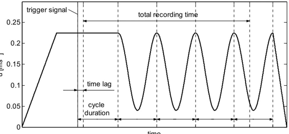
and a defined number of disc rotations is reached, the program will start the transient velocity pattern, triggers the high speed camera and records data; e.g. the traction force acting on the specimen, the temperatures measured by the thermalcouples close to the contact and voltage output of the tachometers and encoders. Finally, after running the desired amount of test cycles, the control program slows down the disc and specimen until the test rig stops. In Figure 2-4 an exemplary test run is shown.
0 0.05 0.1 0.15 0.2 0.25 u [ m s -1 ] time
total recording time
time lag cycle duration trigger signal
Figure 2-4: Entraining velocity over time as applied in the transient experiments.
2.2.1 Data acquisition
Two standard PC’s were utilized for the control setup. A Pentium II computer controlled the test rig. As a soft- and hardware, LabView® (Version 5) and a National Instrument® card (AT-MIO-16E-10) with the corresponding Data Acquisition Board (DAQ board SC-2345) were used. The other computer (Pentium IV) was connected to the high speed camera via a FireWire (IEEE 1394) interface. Another solution could have been to use one computer for both, the high speed camera and the National Instrument® hard- and software. This however leads to compatibility problems with the National Instrument® equipment used in this work. Furthermore, due to the high amount of pictures generated by the high speed camera it is convenient to have one computer for the image processing and storing, and another for controlling the
test rig and data acquisition (tachometer and encoder voltage, temperatures, traction forces, etc.).
For all possible test frequencies the sample rate was always set to be high enough that aliasing effects could be excluded. Compared to steady state conditions under transient conditions the sample rate has to be higher. However, the operation time of a standard PC is limited. This means for high sample rates the amount of data was higher than the amount that could be real time operated. Therefore, the data were stored first (“buffer” – no delay) and after a defined recording interval processed (e.g. the averaging operation was done).
The high speed CMOS camera (model 1200 HS manufactured by PCO AG, Germany) itself was controlled by the PCO AG CamWare® software. A speed of up to 636 frames per second at its maximum resolution of 1280×1024 pixels and a color depth of 30 bits can be reached. This is possible due to an internal memory of 4 GB. After recording, the images were transferred via the FireWire interface to the PC for further processing.
2.2.2 Camera trigger
During experiments under changing speed, within seconds, a huge amount of images will be generated. If the kinematic conditions change over time (in our case the speed) it will be somehow troublesome to select representative images for analysis purpose.
Therefore the high speed camera is started by a trigger signal in order to relate every image to the corresponding speed. For this purpose a rotary encoder connected to the shaft of the disc with two channels A and B is used. Channel A sends a TTL signal for a given increment (depending on the encoders accuracy) whereas channel B sends one TTL signal for each complete rotation of the encoder. After some filtering with an electronic circuit, the two TTL signals are connected with the input to the integrated counters on the National Instrument® board. Thus, it is possible to correlate the position of the disc with the encoder signal. Channel B is important to reset the signals counted for one encoder rotation. This is necessary in order to minimize the accumulation of counting errors with every rotation. Even if only an error of one increment for each rotation
occurs, without the use of Channel B the error would add up and consequently would make it impossible to locate the exact position of the disc.
After the maximum test speed is reached and a defined integer number of disc revolutions (Figure 2-5), a trigger signal to start the high speed camera is sent.
Figure 2-5: Parameter input for the high speed camera trigger.
As shown schematically in Figure 2-4, a time lag between the trigger signal and the actual acquisition of the first image was inevitable (e.g. due to the operation time of the computers, electrical circuits etc.). The time delay is relatively small and in a range of about 50 ms. However, when testing for higher frequencies the time lag must be determined in order to locate the correct images to the continuously changing speed. A similar discussion is reported in Ren [74].
As an example, let us assume a test frequency of 1 Hz and a frame rate of 1000 images per cycle. For a assumed time delay of 0.05 s theoretically 50 images will pass before the camera has even recorded the first image. Without the consideration of the time lag the shift of 50 images can lead to wrong interpretations when analyzing them. For higher test frequencies the shift would be even higher, whereas for low test frequencies the time lag can be neglected. Knowing the exact position of the disc, the time lag can be simply estimated by placing a black mark on the upper side of the disc (Figure 2-6).
Figure 2-6: Template to measure the time delay (schematically).
Prior to starting each experiment, the leading edge of the mark was positioned in the field of vision of the high speed camera. The trigger signal was activated after an integer number of disc revolutions and exactly one cycle duration before the beginning of the sinusoidal speed profile (see Figure 2-4). Thus, every recording contained one steady state cycle and several transient cycles. Knowing the recording frame rate and the theoretical number of dark images caused by the black mark passing by the camera’s field of vision, one can determine the time lag from the actual number of dark images at the beginning of a recording. The time lag is simply the number of dark images already passed divided by the frame rate. For more explanations the reader is referred to [18] and [19].
2.2.3 High speed camera
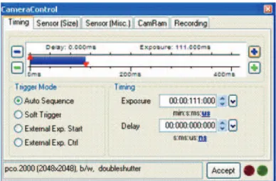
As already stated above, the camera settings are defined by the software CamWare®. After some test runs it was found that the frame rate needs to be adjusted. This kind of problem may depend on the equipment used, e.g. the high speed camera itself or the corresponding software. However, it is worth to give some explanations, since similar problems may occur in other applications if a high speed camera is in use.
As an example, for experiments carried out with a test frequency of 1 Hz a frame rate of 500 images/s was chosen. For this purpose the exposure time of the high speed camera is set to 2 ms. In Figure 2-7 is shown the control window of the PCO AG CamWare® software.
Figure 2-7: Control window for setting the exposure time and delay time (frame rate regulation).
Therefore one will record for 1-cycle and 1 s exactly 500 images. For a lower test frequency of 0.25 Hz, 1-cycle will be 4 s long. In order to have the same number of images for 1-cycle one needs to set the frame rate in such a way that only 125 images per second will be recorded. Increasing simply the exposure time to 8 ms will fail, because the images will be overexposed. In addition, the quality of the images would be different compared to the ones recorded for 1 Hz (exposure time 2 ms).
Theoretically one could set a delay time of 6 ms and an exposure time of 2 ms in order to obtain 8 ms. Unfortunately, in this way the frame rate will not give correct results. For example, if the frame rate is set as described, then the time passed between the 1st and the 126th image should be exactly 1 s. This is not the case and consequently, after recording many images under transient conditions, it would be very difficult to find the correct image to the corresponding velocity.
To overcome this problem, a correction time has to be calculated. First the sensor size of the high speed camera needs to be defined for the desired test conditions. (Often, for memory space optimization reasons, it is sufficient to use only a part of the cameras field of vision.)
Let us assume that one wants to calculate a correction time for a test frequency of 0.25 Hz using a frame rate of 500 Images per cycle. Furthermore one wants to record 4 cycles. This results in a total amount of 2000 images after 16 s. (The
maximum amount of images which can be recorded by the high speed camera changes depending on the sensor size and cam ram set.)
In order to calculate the correction time a test run is necessary. First, the frame rate is set as described above to a total trigger time of 8 ms. In other words, a delay time of 6 ms and an exposure time of 2 ms is set. The results of the test run are summarized in Table 2-1.
Table 2-1: Results for a delay time of 6 ms and an exposure time of 2 ms.
16 14.222059 54.541167 2001 0 0 40.319108 1 Theoretical Time [s] Actual Time [s] Time Indicator [s] Image
The difference between the theoretically expected time after 16 s and the actual time is nearly 2 s. This is a big error considering a frame rate of 125 images per second. Knowing the results above, the correction can be calculated as following
max max t Delay Exposure I = − ( 2-3 )
where tmax is the maximum time measured, Imax the corresponding image number, and “Exposure” the exposure time set. Thus,
14.222059
0.002 0.00510747576 2001
Delay = − = s
Therefore, the correction time will be
6 5.10747576 0.89252
theoretical
Correction=Delaytime −Delay = ms− ms= ms
Adding this correction time to the delay time one will obtain a correct frame rate as shown in Table 2-2. It can be seen that, including the correction time the error during the registration of 2000 images in 16 s is negligible.
Table 2-2: Results for a delay time of 6 ms+correction and an exposure time of 2 ms. 16 16.003753 32.375683 2001 12 12.002815 28.374745 1501 8 8.001876 24.373806 1001 4 4.000938 20.372868 501 1 1.000234 17.372164 126 0 0 16.371930 1 Theoretical Time [s] Actual Time [s] Time Indicator [s] Image Exposure time: 2ms Delay time: 6ms+0.89252ms
Another solution could be the additional use of an external signal generator. For the application explained here two external signals would be necessary. One signal needs to trigger every single picture of the high speed camera and another signal needs to define the time of exposure. In this work, however, such a signal generator was not available.
2.3
Analysis of the friction coefficients under transient
conditions
With the test rig explained above, basically the film thickness and the friction force were measured. Here, a short description of the procedure in analyzing the friction data obtained under transient conditions is given. A detailed explanation of the test conditions and experimental results is not intended in this section. As mentioned before, the friction force was measured by a load cell which constricts the axial movement of a gas bearing that supports the rotating shaft of the test rig. Compared to experiments carried out under steady state conditions the influence of noise (e.g. vibrations) becomes more evident under transient conditions. Furthermore under transient conditions the sample rate is higher. However, the operation time of a standard PC is limited. For high sample rates the amount of data was higher than the amount that could be operated. Therefore the raw data were stored (“buffer”) and after a defined recording interval the average operation was taken. The pre-averaged data still contain a lot of noise. In order to get rid of the high amount of noise, further average operations and filtering is necessary. For this purpose Matlab® was used.
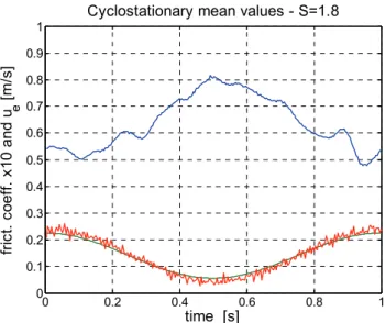
In general, good results have been obtained when averaging the measured data of several cycles. This means at least 20 cycles for friction force measurements under transient conditions have been recorded. In Figure 2-8, the results for the friction coefficients of a complete cycle after averaging 20 cycles (referred to as cyclostationary mean) can be seen. Also, the measured (red line) and theoretical (green line) mean entraining velocity ue is present. For this test the mean speed was changed with a sinusoidal law at a test frequency of 1 Hz between 0.055 m/s and 0.225 m/s. As evident the velocities show some fluctuation but correspond well with the theoretical speed. The friction coefficients show big fluctuations even after averaging 20 cycles.
0 0.2 0.4 0.6 0.8 1 0 0.1 0.2 0.3 0.4 0.5 0.6 0.7 0.8 0.9
1 Cyclostationary mean values - S=1.8
time [s] fr ic t. c oef f. x 10 and u e [m /s]
Figure 2-8: Full cycle of an averaged friction coefficient over time (test frequency of 1 Hz, S=1.8).
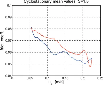
In Figure 2-9 the friction coefficient values are illustrated over the mean velocity. A difference in the friction coefficient values is found for accelerating (red line) and decelerating (blue line) speeds. This is due to transient effects and will be explained more in chapter 4. The occurrence of such so-called friction coefficient loops depends on the test conditions in non-steady state experiments and is reported also in other works like Hess et al [46].
0 0.05 0.1 0.15 0.2 0.25 0.04 0.05 0.06 0.07 0.08 0.09
0.1 Cyclostationary mean values S=1.8
ue [m/s] fr ic t. co ef f.
Figure 2-9: Full cycle of an averaged friction coefficient over mean velocity (test frequency of 1 Hz, S=1.8).
To sum up, in the cyclostationary mean cycle the fluctuations in the friction coefficient values are still relatively strong and show the need of further processing.
Thus, the cyclostationary mean cycle was high pass filtered by using the Fourier transform algorithm. For the filtering purpose the use of the mean cycle (see Figure 2-9) gave best results. Figure 2-10 shows the frequency spectrum of the raw friction coefficient data. Several peaks in a frequency range between 0 and 30 Hz are present. High pass filtering was carried out in the simple way that the FFT of the recorded signals is made, then the values corresponding to frequencies greater than a specified one (referred to as cutting frequency) are put to zero and the inverse transform is finally made. After many test runs it was figured out that, good results are obtained when using a cutting frequency which is 1.5 times the test frequency, or a cutting frequency which corresponds to the greatest rotation frequency of disc and specimen [17].
0 5 10 15 20 25 30 35 40 0.002 0.004 0.006 0.008 0.01 0.012 0.014 0.016 0.018 Amplitude S=1.8 frequency [Hz] am pl itude
Figure 2-10: FFT spectrum of the friction coefficient signal.
In Figure 2-11 are shown the raw friction coefficient data together with the filtered data for all 20 cycles. The necessity in averaging and filtering the friction data is very clear. It would be impossible to interpret results obtained in non-steady state experiments by just looking on the raw friction data.
Figure 2-11: Raw and filtered data over speed.
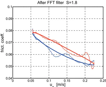
The final result of the present example is shown in Figure 2-12. For comparison reasons, the friction coefficient data after FFT filtering of the cyclostationary mean cycle and the unfiltered cyclostationary mean cycle are plotted together.
All told it can be seen that the filtering of a cyclostationary mean cycle, based on a sufficiently high number of cycles (in our case 20 cycles), with a cutting frequencies 1.5 times the test frequency, provides results suitable for comparisons not influenced by unwanted vibration effects.
0 0.05 0.1 0.15 0.2 0.25 0.04 0.05 0.06 0.07 0.08 0.09 0.1 After FFT filter S=1.8 ue [m/s] fr ic t. co ef f.
Figure 2-12: Friction coefficient data after FFT filtering and cyclostationary mean values (test frequency of 1 Hz, S=1.8).
CHAPTER 3
MEASUREMENT OF THE FILM THICKNESSES
During experiments under transient conditions, in order to analyze fast events, a big amount of interferogram images must be recorded. So far there was no possibility at the DIMNP to analyze large numbers of interferograms efficiently. Considering this situation, it was self-evident that the development of new or improved image processing programs could enhance the explanatory power of measurement results and above all reduce the time needed to obtain these results.
3.1 Existing solution at the DIMNP
Prior to the present work, at the DIMNP there were already some programs to analyze monochromatic interferograms in two dimensions, as the one described in [16]. Apart from the fact that this program did not run without modifications on more recent versions of Matlab®, it required the user to manually define a number of points from where the fringes were counted in different directions. Squarcini [80] presented a similar, but more sophisticated program based on phase unwrapping instead of fringe counting. This program could take into account shades of gray between the extremes of monochromatic interferograms, but still required subdivision of the image into several zones, which were processed in different ways.
Considering this expenditure of inputs and the limited suitability of monochromatic interferograms for transient experiments, further improvements of these programs did not seem promising.
So far the white light interferograms generated during experiments under transient condition needed to be analyzed by eye. To give someone an idea, a comparison between some exemplary outputs of the new image processing program with the manual image analysis method is demonstrated in Figure 3-1. With the previous method mostly the minimum and central film thickness was
determined from white light interferograms. A detailed description of the new image processing program will be given later.
Like the new program, the manual method employs a calibration table. This table relates a qualitative description of colors to film thicknesses. The table presented here is discretized in varying steps between 30 nm and 90 nm, consequently offering a resolution similar to a monochromatic interferogram analysis program. However, the accuracy depends also on the individual color perception of the person using the table.
-1500 -100 -50 0 50 100 150 0.1 0.2 0.3 0.4 0.5 0.6 y [μm] film th ic kn e ss [μ m] 0.95 purple 0.86 green 0.75 purple 0.66 green 0.59 purple 0.53 yellow 0.46 green 0.42 blue 0.39 purple 0.36 orange 0.33 yellow 0.30 green 0.24 blue 0.21 purple 0.18 orange 0.14 yellow 0.10 white <0.02 black FILM THICKNESS (μm) COLOR 0.95 purple 0.86 green 0.75 purple 0.66 green 0.59 purple 0.53 yellow 0.46 green 0.42 blue 0.39 purple 0.36 orange 0.33 yellow 0.30 green 0.24 blue 0.21 purple 0.18 orange 0.14 yellow 0.10 white <0.02 black FILM THICKNESS (μm) COLOR
Figure 3-1: Comparison of film thicknesses determined with the image analysis program and by manual table lookup (table for a refractive index of 1.5, according to [14], interferogram recorded under steady-state conditions,
ball Ø = 10.319mm, S = 0.25, ue = 0.25 ms-1).
In the present example, the color in the area where the minimum film thickness occurs can be described as a greenish yellow. Note that the color perceived by the eye differs between the two side lobes, probably due to non-uniform illumination. However, the value seems to be almost the same, since a film
![Figure 1-2: Pressure profile and film thickness of a typical EHL contact (source: [http://www.ime.rwth-aachen.de,2003])](https://thumb-eu.123doks.com/thumbv2/123dokorg/7333501.91104/17.748.167.612.102.483/figure-pressure-profile-thickness-typical-contact-source-aachen.webp)
![Figure 1-3: Effect of the elastic deformation and viscosity on EHL film generation (source: [http://www.ime.rwth-aachen.de,2003])](https://thumb-eu.123doks.com/thumbv2/123dokorg/7333501.91104/18.748.102.584.267.537/figure-effect-elastic-deformation-viscosity-generation-source-aachen.webp)