UNIVERSIT `
A DI BOLOGNA
SCUOLA DI INGEGNERIA E ARCHITETTURA CAMPUS DI CESENA
CORSO DI LAUREA MAGISTRALE IN INGEGNERIA E SCIENZE INFORMATICHE
APPLYING THE REACTIVE PROGRAMMING
PARADIGM: TOWARD A MORE DECLARATIVE
APPLICATION DEVELOPMENT APPROACH
Elaborata nel corso di: Programmazione Avanzata e Paradigmi
Supervisor:
Prof. ALESSANDRO RICCI Co-supervisor:
Prof. PHILIPP HALLER
Student: ALESSANDRO ZOFFOLI
ACADEMIC YEAR 2014–2015 SESSION I
Reactive Programming Declarative Streams State Side effects
Introduction xi
1 Reactive programming 1
1.1 Functional Reactive Programming . . . 2
1.1.1 Behaviors and Event Streams . . . 3
1.2 Evaluation model . . . 4
1.3 Glitches . . . 6
1.4 Lifting . . . 8
1.5 Reactive confusion . . . 9
2 State of the union 11 2.1 Scala.React . . . 11 2.1.1 Reactive . . . 12 2.1.2 Evaluation model . . . 15 2.2 RxJava . . . 16 2.2.1 Observable . . . 16 2.2.2 Subscription . . . 24 2.2.3 Scheduler . . . 25 2.2.4 Subject . . . 26 2.2.5 RxAndroid . . . 29 2.3 ReactiveCocoa . . . 30
2.3.1 Event and Signal . . . 31
2.3.2 ProperyType . . . 36
2.3.3 Action . . . 37
2.4 Akka Streams . . . 38
2.4.1 Source . . . 39
3 Towards reactive mobile application development 47 3.1 Abstracting the retrieval, manipulation and presentation of
data . . . 47
3.1.1 On Android . . . 48
3.1.2 On iOS . . . 51
3.2 Choosing an architectural pattern . . . 52
3.2.1 State of the art in iOS . . . 52
3.2.2 State of the art in Android . . . 55
3.2.3 Toward a common architecture: MVVM . . . 55
3.3 A case study . . . 57
3.3.1 A common architecture . . . 57
3.3.2 Implementation on Android . . . 60
3.3.3 Implementation on iOS . . . 71
3.3.4 Considerations . . . 78
4 Towards reactive event processing 79 4.1 Building a processing pipeline: a case study . . . 79
4.1.1 Implementation on Akka streams . . . 80
4.2 Implementation on RxScala . . . 87
4.2.1 Considerations . . . 90
5 A conclusive comparison 91 5.1 Operators, Expressions, Declarativness . . . 91
5.2 Hot and Cold, Push and Pull, Back-pressure . . . 92
5.3 Solving problems the reactive way . . . 93
A Functional Programming 95 A.0.1 Entities and value objects . . . 95
A.0.2 Services . . . 96
A.1 Algebraic data types . . . 96
A.2 ADTs and Immutability . . . 99
A.3 Referential trasparency . . . 102
A.3.1 Equational reasoning . . . 103
A.4 Patterns . . . 103
B Future and Promises 111 B.1 Futures . . . 112 B.2 Promises . . . 115 C Reactive Streams 117 C.1 Subscriber . . . 119 C.2 Subscription . . . 120 C.3 Publisher . . . 120 C.4 Processor . . . 121
After almost 10 years from “The Free Lunch Is Over” article, where the need to parallelize programs started to be a real and mainstream issue, a lot of stuffs did happened:
• Processor manufacturers are reaching the physical limits with most of their approaches to boosting CPU performance, and are instead turning to hyperthreading and multicore architectures;
• Applications are increasingly need to support concurrency;
• Programming languages and systems are increasingly forced to deal well with concurrency.
The article concluded by saying that we desperately need a higher-level programming model for concurrency than languages offer today.
This thesis is an attempt to propose an overview of a paradigm that aims to properly abstract the problem of propagating data changes: Reactive Programming (RP). This paradigm proposes an asynchronous non-blocking approach to concurrency and computations, abstracting from the low-level concurrency mechanisms.
The first chapter of this thesis will introduce the basics of RP, starting from simple abstractions and then exploring their main advantages and drawbacks.
The second chapter will present a detailed overview of some of the most popular and used frameworks that enable the developer to put RP principles in practice. This chapter will present the main abstractions and APIs for each framework, with a particular attention for the style and approach that the framework itself suggests in respect to the host language used.
and Android as the reference platforms, and will then explore a common architectural approach to better express and implement mobile applications. It won’t be a surprise that RP will have a central role in this chapter.
The fourth chapter will propose an approach to implement event pro-cessing application. This kind of applications will have an increasing role in our days, and RP expressiveness can be useful to model and express applications that interact and compute a lot of real-time data.
Finally, the fifth chapter will conclude the thesis, with some final note and comparison.
Reactive programming
When using the imperative programming paradigm, the act of capturing dynamic values is done only indirectly, through state and mutations. In this context, the idea of dynamic/evolving values is not a first class value in the paradigm. Moreover, the paradigm can only capture discrete evolving values, since the paradigm itself is temporally discrete.
Reactive programming is a programming paradigm that aims to provide a more declarative way to abstract computations and mutations.
Wikipedia defines reactive programming as:
a programming paradigm oriented around data flows and the propagation of change. This means that it should be possible to express static or dynamic data flows with ease in the program-ming languages used, and that the underlying execution model will automatically propagate changes through the data flow. In this definition emerges some key concepts:
• expressing computations in terms of data flows • change is propagated in a composable way
• the language or framework has to support declarativeness
• all the “plumbing work” is done by the execution model, ensuring that the actual computation respects the semantics
One of the best examples to describe reactive programming is to think of a spreadsheet, in which there’re three cells, A, B and C and A is de-fined as the sum of B and C. Whenever B or C changes, A updates itself.
The example is really simple and it’s also something that we’re used to know. Reactive programming is all about propagating changes throughout a system, automatically.
This chapter will focus on Functional Reactive Programming and Reactive Programming, in an attempt to provide formal definitions.
1.1
Functional Reactive Programming
Functional reactive programming has its origin with Fran (Functional re-active animation), a Haskell library for interre-active animations by Conal Elliott. Elliott found it difficult to express the what of an interactive ani-mation abstracting from the how, and built a set of expressive and recursive data types, combined with a declarative programming language.
Informally, functional reactive programming is a programming paradigm that brings a notion of time in the functional programming paradigm, pro-viding a conceptual framework for implementing reactive systems. In fact, FRP let the application achieve reactivity by providing constructs for spec-ifying how behaviors change in response to events.
Elliott says that FRP is all about two main things: denotative and temporally continuos. Infact, he also likes the term “denotative, continuous-time programming” to replace functional reactive programming, since it reduces the confusion.
Always about the denotative part, he means that the paradigm should be founded on a precise, simple, implementation-independent, composi-tional semantics that exactly specifies the meaning of each type and build-ing block. The compositional nature of the semantics then determines the meaning of all type-correct combinations of the building blocks.
From an Elliott’s quote:
Denotative is the heart and essence of functional programming, and is what enables precise and tractable reasoning and thus a foundation for correctness, derivation, and optimization.
About the continuous time part, there’s some confusion. Some claim that it’s an idea somehow unnatural or impossible to implement considering the discrete nature of computers. To these issues, Elliott answers in the following way:
This line of thinking strikes me as bizarre, especially when com-ing from Haskellers, for a few reasons: Uscom-ing lazy functional languages, we casually program with infinite data on finite ma-chines. We get lovely modularity as a result [. . . ]. There are many examples of programming in continuous space, for in-stance, vector graphics, [. . . ] I like my programs to reflect how I think about the problem space rather than the machine that executes the programs, and I tend to expect other high-level language programmers to share that preference.
Another name that Elliott suggests for continuous is resolution-independent, and thus able to be transformed in time and space with ease and without propagating and amplifying sampling artifacts. As an example, he proposes the “finite vs infinite” data structure issue:
We only access a finite amount of data in the end. However, allowing infinite data structures in the middle makes for a much more composable programming style. Each event has a stream (finite or infinite) of occurrences. Each occurrence has an asso-ciated time and value.
Fran integrates general ideas from synchronous data-flow languages into the non-strict, pure functional language Haskell. It takes a monadic ap-proach and encapsulates operations over time-varying values and discrete events into data structures that are evaluated by an interpreter loop. The main idea of FRP is to model user inputs as functions that change over time.
1.1.1
Behaviors and Event Streams
FRP introduces two special abstractions:
• behaviors or signals, values that are continuous functions of time. • event streams, values which are discrete functions of time.
Behaviors are dynamic/evolving values, and are first class values in themselves. Behaviors can be defined and combined, and passed into and out of functions.
Behaviors are built up out of a few primitives, like constant (static) behaviors and time (like a clock), and then with sequential and parallel combination. n-behaviors are combined by applying an n-ary function (on static values), “point-wise”, i.e., continuously over time.
In other terms, a Behavior simply sends values over time until it either completes, or errors out, at which point it stops sending values forever.
Examples of behaviours are the following: • time
• a browser window frame • the cursor position
• the position of an image during an animation • audio data
• . . .
Events enable to account for discrete phenomena, and each of it has a stream (finite or infinite) of occurrences. Each occurrence is a value paired with a time. Events are considered to be improving list of occurrences.
Formally, the points at which an event stream is defined are termed events and events are said to occur on an event stream.
Examples of event streams are the following: • timer events • key presses • mouse clicks • MIDI data • network packets • . . .
Every instance of FRP conceptually includes both behaviors and events. The classic instance of FRP takes behaviors and events as first-class values.
1.2
Evaluation model
The core of languages that support Reactive Programming is about how changes are propagated. From the programmer’s point of view this
should be as much transparent as possible. In other words, a change of a value is automatically propagated to all dependent computations without the user has to manually propagate the changes by himself.
At the language level this means that there should be a mechanism that is triggered when there’s an event occurrence at an event source. This mech-anism will fire a notification about the changes to dependent computations that will possibly trigger a recomputation, and so on.
The issue of who initiates the propagation of changes is a really impor-tant decision in designing a language or a framework that supports RP.
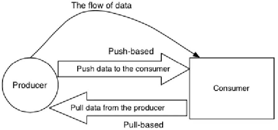
In simple terms the question is whether the source should push new data to its dependents (consumers) or the dependents should pull data from the event source (producer).
Figure 1.1: Push- Versus Pull-based evaluation model, from the paper “A survey on Reactive Programming”
In the literature there are two main evaluation models:
• Pull-Based, in which the computation that requires a value has to pull it from the source. The propagation is said to be demand-driven. The pull model has been implemented in Fran, also thanks to the lazy evaluation of Haskell. A main trait of this approach is that the computation requiring the value has the liberty to only pull the new values when it actually needs it. From another point of view, this trait can lead to a significant latency between an occurrence of an event and when its reactions are triggered.
• Push-Based, in which when the event source has new data it pushes the data to its dependent computations. The propagation is said to be data-driven. An example of a recent implementation that uses this model is Scala.React, that will be introduced later in this thesis. This approach also brings the issue of wasteful recomputation, since every new data that is pushed to the consumer triggers a recomputation. Typically, reactive programming languages use either a pull-based or push-based model, but there are also languages that employ both ap-proaches. In latter case there’ve both the benefits of the push-based model (efficiency and low latency) and those of the pull-based model (flexibility of pulling values based on demand).
1.3
Glitches
A glitch is a temporary inconsistency in the observable state. Due to the fact that updates do not happen instantaneously, but instead take time to compute, the values within a system may be transiently out of sync during the update process. This may be a problem, depending on how tolerant the application is of occasional stale inconsistent data. For example, consider a computation that is run before all its dependent expressions are evaluated and that can result in fresh values being combined with stale values.
The paper “A Survey on Reactive Programming” by Bainomugisha et al. depict the problem with the following program:
var1 = 1
var2 = var1 * 1 var3 = var1 + var2
The image related to the program above shows how the state of the program results incorrect (var3 is evaluated as 3 instead of 4) and that this also leads to a wasteful recomputation (since var3 is computed one time more than the necessary).
Glitches only happen when using a push-based evaluation model and can be avoided by arranging expressions in a topologically sorted graph. This implementation detail ensures that an expression is always evaluated after all its dependants have been evaluated.
Figure 1.2: Momentary view of inconsistent program state and recomputa-tion.
1.4
Lifting
The term lifting is used to depict the process of converting an ordinary operator to a variant that can operate on behaviors. This process is essential for the end user of the language/framework, since it ensures conciseness and composability. In other words, lifting is used to move from the non-reactive world to reactive behaviors.
Lifting a value creates a constant behavior while lifting a function applies the function continuously to the argument behaviors. There is no similar lifting operation for events, since an event would need an occurrence time as well as a value.
Lifting an operation can be formalized by the following definition, as-suming functions that only take one parameter (generalising to functions that take multiple arguments is trivial):
lif t : f (T ) → flif ted(Behavior < T >).
The flif ted function can now be applied to behaviors that holds values of
type T . Lifting enables the language or framework to register a dependency graph in the application’s dataflow graph.
Starting from the previous definition, the evaluation of a lifted function called with a behavior at the time step i can be formalized as follows:
flif ted(Behavior < T >) → f (Ti).
where Ti is the value of the behavior at the time step i.
In the literature there are at least three main lifting strategies:
1. Implicit lifting, that happens when an ordinary language operator is applied on behaviour and it is automatically lifted. Dynamically typed languages often use implicit lifting. Formally:
f (b1) → flif ted(b1).
2. Explicit lifting, usually used by statically typed languages. In this case the language provides a set of combinators to lift ordinary oper-ators to operate on behaviors. Formally:
3. Manual lifting, when the language does not provide lifting operators. Formally:
f (b1) → f (currentV alue(b1)).
1.5
Reactive confusion
In these days reactive programming and functional reactive pro-gramming are two terms that create a lot of confusion, and maybe are also over-hyped.
The definitions that come from Wikipedia are still pretty vague and only FRP introduced by Connal Elliott has a clear and simple denotative semantics. In advance to this, Elliott himself doesn’t like the name he gave to the paradigm.
The concepts behind these newly introduced paradigms are pretty simi-lar. Reactive programming is a paradigm that facilitates the development of applications by providing abstractions to express time-varying values and automatically propagating the changes: behaviors and events. Functional reactive programming can be considered a “sibling” of reactive program-ming, providing composable abstractions. Elliot identifies the key advan-tages of the functional reactive programming paradigm as: clarity, ease of construction, composability, and clean semantics.
In 2013 Typesafe launched http://www.reactivemanifesto.org, which tried to define what reactive applications are. The reactive manifesto didn’t in-troduce a new programming paradigm nor depicted RP as we intended RP in this thesis. What the reactive manifesto did instead was to depict some really relevant computer science principles about scalability, resilience and event-driven architectures, and RP is one of the tools of the trade.
Erik Meijer, in his talk “Duality and the End of Reactive”, concluded that all the hype and the buzzwords around the “reactive world” has no sense, and that the core of the paradigm is all about composing side effects. In his talk and related papers, he depicted the duality that links enumerables and observables.
In short, an enumerator is basically a getter with the ability to fail and/or terminate. It might also return a future rather than a value. An iterable is a getter that returns an iterator. If we take the category-theoretic dual of these types we get the observer and observable types.
Table 1.1: The essential effects in programming One Many
Synchronous T/Try[T] Iterable[T] Asynchronous Future[T] Observable[T]
And this conclusion is what let us to relate all the principal effects in pro-gramming, where in one axis there’s is the nature of the computation (sync or async) and in the other one there’s the cardinality of the result (one or many).
State of the union
The previous chapter quickly introduces the basic notions of RP. This chap-ter will give an overview of the state of the art for RP frameworks.
This thesis author arbitrarily choose four relevant libraries:
• Scala.React • RxJava
• ReactiveCocoa • Akka Streams
2.1
Scala.React
Scala.React is a framework that has been introduced with the paper “Dep-recating the Observer Pattern” from Maier, Odersky and Rompf. The key concepts around Scala.React originate in Elliot’s FRP, and Scala.React aims to provide a combinator-based approach for reactive programming. The paper depicts how the observer pattern should be considered an anti-pattern, since it violates a lot of software engineering principles such as encapsulation, composability, separation of concerns, scalability, uniformity, abstraction, semantic distance..
The authors aims to provide and depict an efficient use of object-oriented, functional, and data-flow programming principles to overcome the limita-tions of the existing approaches.
After many years from its presentation, the framework seems to be an academic library that can be neglectable in favor of the RxScala/RxJava
library. For the author of this thesis, the paper is really meaningful in the context of this thesis, since it introduces a set of abstractions that are close to the original model of FRP from Elliot.
2.1.1
Reactive
Following the idea to provide APIs that starts with basic event handling and ends in an embedded higher-order dataflow language, the framework introduces a generic trait Reactive, that factors out the possible concrete abstractions in the following way:
trait Reactive[+Msg, +Now] {
def current(dep: Dependant): Now
def message(dep: Dependant): Option[Msg] def now: Now = current(Dependent.Nil) def msg: Msg = message(Dependent.Nil) }
The trait Reactive is defined based on two type parameters: one for the message type an instance emits and one for the values it holds. Starting from the previous base abstraction, two further types can be defined:
trait Signal[+A] extends Reactive[A,A] trait Events[+A] extends Reactive[A,Unit]
The difference between the two types can be seen directly in the types: • In Signal, Msg and Now types are identical.
• In Events, Msg and Now types differ. In particular, the type for the type parameter Now is Unit. This means that for an instance of Events the notion of “current value” has no sense at all.
The two subclasses need to implement two methods, which obtain reac-tive’s current message or value and create dependencies in a single turn.
The next two sections will better examine the two abstraction introduced here.
NB: the examples and code provided in this chapter have been taken directly from the paper itself.
Events
The first type to take in consideration is the Event type.
To simplify the event handling logic in an application, the framework provides a general and uniform event interface, with EventSource. An EventSource is an entity that can raise or emit events at any time. For example:
val es = new EventSource[Int] es raise 1
es raise 2
To attach a side-effect in response to an event, an observer has to ob-serve the event source, providing a closure. Continuing with the previous example, the following code prints all events from the event source to the console. val ob = observe(es) { x => println("Receiving " + x) } ... ob.dispose()
observe( ) returns an handle of the observer,that can be used to unin-stall and dispose the observer prematurely, via its dispose() method. This is a common pattern in all of the other frameworks/libraries presented in this thesis.
The basic types for events handling are pretty neat and simple to reason about, since they are first-class values. The usage of these types starts to be helpful only if combined with a set of operators, that enables developers to build better and declarative abstraction.
For example, the Events trait defines some common operators as follows:
def merge[B>:A](that: Events[B]): Events[B] def map[B](f: A => B): Events[B]
def collect[B](p: PartialFunction[A, B]): Events[B]
When building abstractions, the developer doesn’t need to take care of the events propagation, since the framework itself provides this.
Signal
The Signal type represents the other half of the story.
In programming a large set of problems is about synchronizing data that changes over time, and signals are introduced to overcome these needs.
In simple words, a Signal is the continuous counterpart of trait Events and represents time-varying values, maintaining:
• its current value
• the current expression that defines the signal value
• a set of observers: the other signals that depend on its value
A concrete type for Signal is the Var, that abstract the notion of vari-able signal and is defined as follows:
class Var[A](init: A) extends Signal[A] { def update(newValue: A): Unit = ... }
A Var’s current value can change when somebody calls an update( ) operation on a it or the value of a dependant signal changes.
Constant signals are represented by Val:
class Val[A](value: A) extends Signal[A]
To compose signals, the framework doesn’t provide combinator methods at all, but introduce the notion of signal expressions, indeed. To better explain the concept, let’s look at a simple example.
val a = new Var(1) val b = new Var(2)
val sum = Signal{ a()+b() }
observe(sum) { x => println(x) }
a()= 7 b()= 35
Signals are primarily used to create variable dependencies as seen above. In other words, the framework itself already performs all the “plumbing work” of connecting the dependencies and propagating the changes.
The framework and the Scala language provide a convenient and simple syntax to get and update the current value of a Signal, and also to create variable dependencies between signals. For example:
• the code Signal{ a()+b() } creates a dependencies that binds the changes from a and b to be propagated and evaluated in the sum signal • the code a()= 7 is evaluated as a.update(7)
• the framework also provide an implicit converter that enables to create easily Val signals
2.1.2
Evaluation model
Scala.React’s propagation model is push-driven, and uses a topologically ordered dependency graph. This implementation detail ensures that an expression is always evaluated after all its dependants have been evaluated, so glitches can’t happen.
Scala.React proceeds in propagation cycles. The system is either in a propagation cycle or, if there are no pending changes to any reactive, idle. The model of time the system use is a discrete one.
Every propagation cycle has two phases: first, all reactives are synchro-nized so that observers, which are run in the second phase, cannot observe inconsistent data. During a propagation cycle, the reactive world is paused, i.e., no new changes are applied and no source reactive emits new events or changes values.
A propagation cycle proceeds as follows:
1. Enter all modified/emitting reactives into a priority queue with the priorities being the reactives’ levels.
2. While the queue is not empty, take the reactive on the lowest level and validate its value and message. The reactive decides whether it propagates a message to its dependents. If it does so, its dependents are added to the priority queue as well.
Table 2.1: The essential effects in programming One Many
Synchronous T/Try[T] Iterable[T] Asynchronous Future[T] Observable[T]
2.2
RxJava
The table represents a possible classification of the effects in programming. All the theory and the development of the reactive extensions libraries started with an intuition of Erik Meijer, that theorized that iterable/iterator are dual to observable/observer. And this hypothesis is what let us to relate all the principal effects in programming, where in one axis there’s is the nature of the computation (sync or async) and in the other one there’s the cardinality of the result (one or many).
The appendix on futures and promises covers the case of a computa-tion that returns a single value. This chapter will focus on the abstraccomputa-tion of Observables, analyzing RxJava as a case of study.
As the title of the repository states, RxJava is a library for composing asynchronous and event-based programs using observable sequences for the JVM.
The library was heavily inspired by Rx.NET by Microsoft and is de-veloped by Netflix and other contributors. The code is open source and recently, after 2 years of development, has reached the 1.0 version.
RxJava is also conform to the Reactive Streams initiative (see the ap-pendix), and this means that the hard problem of propagating and reacting to back-pressure has been incorporated in the design of RxJava already, and also that it interoperate seamlessly with all other Reactive Streams implementations.
2.2.1
Observable
The fundamental entity of RxJava is the Observable type. An observable is a sequence of ongoing event ordered in time.
An Observable can emit 3 types of item: • values
• completion event
RxJava provides a really nice documentation, with also some graphical diagrams, called marble diagrams.
Figure 2.1: A marble diagram
A marble diagram depicts how a an Observable and an Operator be-have:
• observables are timelines with sequence of symbols
• operators are rectangles, that accepts in input the upper observable and return in output the lower one
In RxJava, an Observable is defined over a generic type T, the type of its values, as follows:
class Observable<T> { ... }
An Observable can emit - in order - zero, one or more values, an error or a completion event.
An Observable is an immutable entity, so the only way to change the sequence of values it emits is through the application of an operator and the subsequent creation of a new Observable.
An entity can subscribe its interest in the values coming from an Observalbe through its subscribe( ) method, that accepts one, two or three Action parameters (that correspond to the onNext( ), onError( ) and onComplete( ) callbacks).
The classic “Hello, World” example in RxJava and Java 8 is the follow-ing:
Observable.just("Hello, world!").subscribe(s -> System.out.println(s));
The Observable type provides some convenience methods that return an observable with the given specification. An incomplete list of these is the following:
• just( ): convert an object or several objects into an Observable that emits that object or those objects
• from( ): convert an Iterable, a Future, or an Array into an Observ-able
• empty( ): create an Observable that emits nothing and then com-pletes
• error( ): create an Observable that emits nothing and then signals an error
• never( ): create an Observable that emits nothing at all
• create( ): create an Observable from scratch by means of a function • defer( ): do not create the Observable until a Subscriber subscribes;
create a fresh Observable on each subscription • . . .
Usually, observables created with these methods are used in conjunction with other observables and operators, to create more complex logics.
Operator
In RxJava, operators are what enable the developer to model the actual computation. An operator allows performing almost every type of ma-nipulation on the source observer in a declarative way.
Expressing a computation in terms of a stream of values is translated in building a chain of proper operators. Usually, looking at the signatures
and at the types of the operators is really helpful when choosing which operator is the right one for the goal to achieve.
An operator, to be applicable to an Observable, has to implement the Operator interface and has to be lifted. The lift function lifts a function (inside an Operator) to the current Observable and returns a new Observ-able that when subscribed to will pass the values of the current ObservObserv-able through the Operator function.
Operators are methods of the Observable class, so creating a chain of operators starting from a source observable is a pretty straightforward process.
RxJava provides a huge set of operators, and a lot of them is defined in terms of other ones. What follows is only a small introductive subset.
Map
Map is an operator that returns an Observable that applies a specified function to each item emitted by the source Observable and emits the results of these function applications. Its marble diagram is the following.
Figure 2.2: Map operator
To better clarify the concept of lifting introduced previously, let’s also look at the definition and implementation for Map.
public final <R> Observable<R> map(Func1<? super T, ? extends R> func) { return lift(new OperatorMap<T, R>(func));
...
public final class OperatorMap<T, R> implements Operator<R, T> {
private final Func1<? super T, ? extends R> transformer;
public OperatorMap(Func1<? super T, ? extends R> transformer) { this.transformer = transformer;
}
public Subscriber<? super T> call(final Subscriber<? super R> o) { return new Subscriber<T>(o) {
public void onCompleted() { o.onCompleted();
}
public void onError(Throwable e) { o.onError(e);
}
public void onNext(T t) { try { o.onNext(transformer.call(t)); } catch (Throwable e) { onError(OnErrorThrowable.addValueAsLastCause(e, t)); } } }; } } FlatMap
FlatMap returns an Observable that emits items based on applying a function that is supplied to each item emitted by the source Observable, where that function returns an Observable, and then merging those resulting Observables and emitting the results of this merger.
Filter
Figure 2.3: FlatMap operator
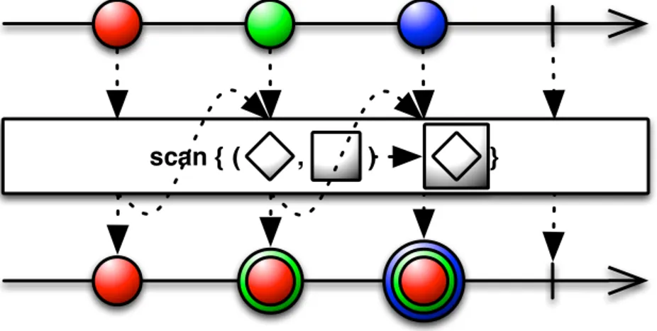
Scan
Scan returns an Observable that applies a specified accumulator function to the first item emitted by a source Observable, then feeds the result of that function along with the second item emitted by the source Observable into the same function, and so on until all items have been emitted by the source Observable, and emits the final result from the final call to your function as its sole item.
Figure 2.5: Scan operator
Take
Take returns an Observable that emits only the first n items emitted by the source Observable.
A complex example
// Returns a List of website URLs based on a text search Observable<List<String>> query(String text) { ... }
// Returns the title of a website, or null if 404 Observable<String> getTitle(String URL){ ... }
query("Hello, world!") // -> Observable<List<String>> .flatMap(urls -> Observable.from(urls)) // -> Observable<String>
.flatMap(url -> getTitle(url)) // -> Observable<String> .filter(title -> title != null)
Figure 2.6: Take operator
// -> Observable<Pair<Integer, String>>
.map(title -> new Pair<Integer, String>(0, title))
.scan((sum, item) -> new Pair<Integer, Word>(sum.first + 1, item.second)) .take(5)
.subscribe(indexItemPair ->
System.out.println("Pos: " + indexItemPair.first + ": title:" + indexItemPair.second ));
The example starts with the hypothesis of having two methods that returns observable, for example coming from the network layer of an appli-cation. query return a list of url given a text and getTitle returns the title of a website or null.
The computation aims to return all the title of the websites that match the “Hello, World!” string.
The code itself is pretty self-explanatory, and shows how concise and elegant a computation can be using the approach suggested by RxJava in respect to its imperative-style counterpart.
Error handling
The previous sections introduced the basics of Observable and Operator. This section will introduce how errors are handled in RxJava.
As introduced previously, every Observable ends with either a single call to onCompleted() or onError().
What follows is an example of a chain of operators that contains some transformation that may also fail.
Observable.just("Hello, world!") .map(s -> potentialException(s))
.map(s -> anotherPotentialException(s)) .subscribe(new Subscriber<String>() {
@Override
public void onNext(String s) { System.out.println(s); }
@Override
public void onCompleted() { System.out.println("Completed!"); }
@Override
public void onError(Throwable e) { System.out.println("Ouch!"); } });
The onError() callback is called if an Exception is thrown at any time in the chain, thus the operators don’t have to handle exceptions in first place since they are propagated to the Subscriber, which has to manage all the error handling.
2.2.2
Subscription
In RxJava, Subscription is an abstraction that represents the link between an Observable and a Subscriber.
A subscription is a quite simple type:
public interface Subscription { public void unsubscribe();
public boolean isUnsubscribed(); }
The main usage for subscription is in its unsubscribe( ) method, that can be used to stop the chain, terminating wherever it is currently executing code.
CompositeSubscription is another useful type, that simplify the man-agement of multiple and related subscriptions. A composite subscription comes with an algebra that defines the behaviors of its methods:
• add(Subscription s), adds a new Subscription to the Compos-iteSubscription; if this is unsubscribed, will explicitly unsubscribing the new Subscription as well
• remove(Subscription s), removes a Subscription from the Com-positeSubscription, and unsubscribes the Subscription
• unsubscribe(), unsubscribes to all subscriptions in the Composite-Subscription
• unsubscribing inner subscriptions has no effect on the composite sub-scription
2.2.3
Scheduler
In the previous sections a lot of concepts have been introduced. This section will cover one of the most important aspects of the framework: schedulers. A scheduler is an object that schedules unit of work, and it’s implemented through the the Scheduler type. This type allows to specify in which execution context the chain or part of the chain has to run. In particular, the developer can choose in which thread:
• an Observable has to run, with subscribeOn( ) • a Subscriber has to run, with observeOn( )
The framework already provide some schedulers:
• immediate( ), that executes work immediately on the current thread • newThread( ), that creates a new Thread for each job
• computation( ), that can be used for event-loops, processing call-backs and other computational work
• io( ), that is intended for IO-bound work, based on an Executor thread-pool that will grow as needed
A really nice feature is the fact that applying the execution of a chain to a particular scheduler doesn’t break the chain of operators, keeping the code clean and with a good level of declarativness.
An example of usage of schedulers is the following, in which an image is fetched from the network and then processed. A network request is a typical io-bound operation and it’s performed in io() scheduler, while a processing operation is a cpu-bound operation and it’s performed in a computation() scheduler. myObservableServices.retrieveImage(url) .subscribeOn(Schedulers.io()) .observeOn(Schedulers.computation()) .subscribe(bitmap -> processImage(bitmap));
2.2.4
Subject
Subject is a further entity that is provided by the framework. A Subject is a sort of bridge or proxy that acts both as an observer and as an Observable:
• because it is an observer, it can subscribe to one or more observ-ables
• because it is an Observable, it can pass through the items it observes by re-emitting them, and it can also emit new items
Subject has the “power” of turning a cold observable hot. In fact, when a Subject subscribes to an Observable, it will trigger that Observable to begin emitting items (and if that Observable is “cold” — that is, if it waits for a subscription before it begins to emit items). This can have the effect of making the resulting Subject a “hot” Observable variant of the original “cold” Observable.
The framework provides a wide range of subjects, each one with its own semantics. What follows is an overview of the main popular and used.
PublishSubject
PublishSubject emits to an observer only those items that are emitted by the source Observable(s) subsequent to the time of the subscription. This means that an observer will not receive the previous emitted items.
Figure 2.7: PublishSubject
ReplaySubject
ReplaySubject emits to any observer all of the items that were emitted by the source Observable(s), regardless of when the observer subscribes. To keep the memory consumption limited, this subject also use a bounded buffer that enable to discard old items when the limit size has been reached.
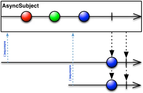
AsyncSubject
Figure 2.9: AsyncSubject
An AsyncSubject caches and only remember the last value of the Ob-servable, and only after that source Observable completes emits that value.
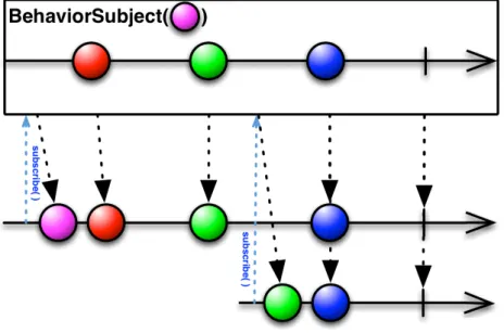
BehaviorSubject
When an observer subscribes to a BehaviorSubject, it begins by emitting the item most recently emitted by the source Observable (or a seed/default value if none has yet been emitted) and then continues to emit any other items emitted later by the source Observable(s).
Figure 2.10: BehaviorSubject
2.2.5
RxAndroid
The previous sections cover all the main topic of RxJava. This section will go a step further, introducing some additional features that bring RxJava to the Android ecosystem.
RxAndroid is a separate module of RxJava that gives some useful bindings to the developer.
The AndroidSchedulers package provides some specific scheduler for the Android threading system.
The additional schedulers provided are:
• AndroidSchedulers.mainThread( ), that will execute an action on the main Android UI thread
• AndroidSchedulers.handlerThread(Handler handler), that uses the provided Handler to execute an action
A typical example of the usage of mainThread( ) is the following, that performs a download in the scheduler io( ) and the show the image to the user:
.subscribeOn(Schedulers.io())
.observeOn(AndroidSchedulers.mainThread())
.subscribe(bitmap -> myImageView.setImageBitmap(bitmap));
ViewObservable is another feature that adds some bindings for an-droid View that returns observables of events that come from the UI, such as:
• clicks( ), that emits a new item each time a View is clicked • text( ), that emits a new item each time a TextView’s text content
is changed
• input( ), same as above, for CompoundButtons • itemClicks( ), same as above, for AdapterViews
These methods are useful to bind the events from the user of an applica-tion, reifying its action and reacting with some operaapplica-tion, in a declarative way.
2.3
ReactiveCocoa
ReactiveCocoa (RAC) is an opensource framework for FRP, developed by Github for the iOS and OS X platforms. RAC has been around for some years now. It started as an Objective-C framework and now it’s object of an almost-complete rewrite using the brand new language introduced by Apple, Swift.
At the time of writing (may/june/july 2015), RAC 3.0 is in beta. The 3.0 version offers new APIs in Swift, that are also mostly backward compatible with version 2.0 (that is written in Objective-C).
Using Swift, the APIs now have a better and cleaner form. In fact, Swift is a language that allows to build composable abstraction pretty easily, sup-porting immutability (value types vs reference types), high-order functions, optionals, custom operators, etc. . .
In the community of iOS and OS X developers RAC is an emerging trend that is clearly gaining the attention of an increasing number of users, confirming the general trend of RP and FRP in our industry.
2.3.1
Event and Signal
The first abstraction that the framework introduces is the notion of event. An event enables to account for discrete phenomena, and each of which has a stream (finite or infinite) of occurrences. Each occurrence is a value paired with a time. Events are considered to be improving list of occurrences. Or, in simpler words, events are things that happen.
In RAC, events are first-class citizens, with the following type:
public enum Event<T, E: ErrorType> { case Next(Box<T>)
case Error(Box<E>) case Completed case Interrupted }
The Event type, taken alone, doesn’t say much. It’s just an enum with some possible related values.
In Swift, an enum is a value type that defines a common type for a group of related values and enables you to work with those values in a type-safe way within your code.
The other fundamental type in RAC is the Signal type, defined as:
public final class Signal<T, E: ErrorType>
A signal is just a sequence of events in time that is conforms to the grammar Next* (Error | Completed | Interrupted)?. The grammar in-troduces a precise semantics and clarify the meaning of the concrete possible instances for the Event type:
• .Next represents an event that carry information of a given type T • .Error represents an event that carry an error of a given type E • .Completed represents a successful terminal event
• .Interrupted represents an event that indicates that the signal has been interrupted
Just like RxJava’s Observable, also RAC’s signal can be distincted in two main categories: hot and cold signals. The main difference from RxJava’s implementation is that in RAC this fundamental distinction can be found di-rectly in the types. In fact, RAC defines Signalas hot and SignalProducer as cold signals.
NB : the previous introduction of Signal is general and applicable on both Signal and SignalProducer.
The next sections will go deeper and explore more on Signals and Sig-nalProducers.
Signal
As introduced previously, Signal implements the abstraction of hot signal as a signal that typically has no start and no end.
A typical practical example for this type can be represented by the press events of a button or the arrival of some notifications. They are just events that happens with no relevance of the fact that someone is observing them.
Using a popular philosophical metaphor:
If a tree falls in a forest and no one is around to hear it, it does make a sound.
Looking at the documentation, a Signal is defined as a push-driven stream that sends Events over time. Events will be sent to all observers at the same time. So, if a Signal has different observers subscribed to its events, every observer will always see the same sequence of events.
The documentation says another crucial thing that clarifies the mod-elling choice made by the developers:
Signals are generally used to represent event streams that are already “in progress”, like notifications, user input, etc. To rep-resent streams that must first be started, see the SignalProducer type.
The RAC’ maintainers decided to keep the distinction between hot and cold Signal at the type level, so RAC offers both the Signal and SignalProducer types.
class Signal<T, E: ErrorType> { ...
}
Signal is parameterized over T, the type of the events emitted by the signal and E, the type that denotes the errors.
A Signal can be created by passing to the initializer a generator clo-sure, which is then invoked with a sink of type SinkOf<Event<String, NoError>>. The sink is then used by the closure to forward events to the Signal through the sendNext( ) method. A similar approach has been implemented also by Akka Streams.
In many cases, a stream of events that has no start and no end can’t terminate with an error. A simple example of this case is a stream of press events from a button. To overcome this possibility, RAC introduces the type NoError, meaning that the signal can’t error out.
For the “button example”, the type for the related signal might be Signal<Void, NoError>, which means:
• the user of the signal only cares about the occurrence of the event, no further information will be provided
• the signal can’t error out, since in this particular case it has no sense to model the fact that a button press can fail
The button example is just one of many others. If we consider the amount of events that come from the UI, a lot of trivial examples come out quickly:
• a signal that models the changes of a text field
• a signal that models the arrival of notifications (remote, local, etc. . . ) • any other signal created combining other signals
• . . .
An example for the creation of a Signal is the following, taken from a blog post of Colin Eberhardt, where a new String is produced every second.
func createSignal() -> Signal<String, NoError> { var count = 0
sink in
NSTimer.schedule(repeatInterval: 1.0) { timer in sendNext(sink, "tick #\(count++)")
}
return nil }
}
To attach some side effect at each Next, Error or Completed event that is produced by a Signal, an observer has to register its interest using observe. The observe operator accepts some closures or functions for any of the event types the user of the API is interested in.
The real deal in using Signals is their power in term of declarativeness when combining Signals with operators to create new Signals to work with. In RAC, all operations that can be applied to signals are simply free functions, in contrast to the “classical-method-definition-on-the-Signal-type approach”. As an example, the map operator signature is defined as follows, with the Signal on which the transformation will be applied passed as an argument:
public func map<T, U, E>(transform: T -> U) (signal: Signal<T, E>) -> Signal<U, E> { ...
}
To keep the APIs fluent RAC also introduces the pipe-forward operator |>, defined as follows:
public func |> <T, E, X>(signal: Signal<T, E>, transform: Signal<T, E> -> X) -> X {
return transform(signal) }
The |> operator doesn’t do anything special, since it only creates a specification.
RAC already offers a numbers of built in operators as free functions, such as combineLatest, zip, takeUntil, concat, . . .
A complete but simple example of usage of all of the aspects introduced is the following:
createSignal()
|> map { $0.uppercaseString } |> observe(next: { println($0) })
The beauty of this approach is that the chain of operations fits the types of each operation, so when the code compiles (and if the user of the APIs has learned the semantics of each operators) the computation acts as expected. All the relevant work for the newcomers of the paradigm consist in taking the time needed to learn the basics and play with the types and the operators.
SignalProducer
The previous section introduced Signal as the type that implements the “hot signal” abstraction. This section will cover the other half of the story. In RAC, “cold signals” are implemented with the SignalProducer type, defined as follows:
public struct SignalProducer<T, E: ErrorType> { ...
}
The generic types are the same as its “hot” counterpart, and also the initializer is pretty similar, with a generator closure:
func createSignalProducer() -> SignalProducer<String, NoError> { var count = 0
return SignalProducer { sink, disposable in
NSTimer.schedule(repeatInterval: 0.1) { timer in sendNext(sink, "tick #\(count++)")
} } }
Using a popular philosophical metaphor, again:
If a tree falls in a forest and no one is around to hear it, it doesn’t make a sound.
Or, in other words, if no one subscribes to the SignalProducer, nothing happens. For SignalProducer, the terminology for subscribing to its events is start( ).
If more than one observer subscribe to the same SignalProducer, the re-sources are allocated for each observer. In the example above, every time an observer invoke the start( ) method on the same SignalProducer instance, a new instance of NSTimer is allocated.
Also on SignalProducers can be applied a wide range of operators. RAC doesn’t implement all the operators twice for Signal and SignalOperator, but it offers a pipe-forward operator that lifts the operators and transformation that can be applied to Signal to also operate on SignalProducer.
The implementation of |>, that applies on the SignalProducer type using Signal’s operator, is the following:
public func |> <T, E, U, F>(producer: SignalProducer<T, E>,
transform: Signal<T, E> -> Signal<U, F>) -> SignalProducer<U, F> { return producer.lift(transform)
}
2.3.2
ProperyType
The previous sections introduced the abstractions that RAC offers to de-scribe signal. This section will introduce other collateral but useful types.
PropertyType is a protocol that, when applied to a property, allows the observation of its changes. Its definition is as follows:
public protocol PropertyType { typealias Value
var value: Value { get }
var producer: SignalProducer<Value, NoError> { get } }
The semantics of this protocol is neat: - the getter return the current value of the property - the producer return a producer for Signals that will send the property’s current value followed by all changes over time
Starting from this protocol, RAC introduces: - ConstantProperty, that represents a property that never change - MutableProperty, that represents
a mutable property - PropertyOf, that represents a read-only view to a property
These types are really usefull when used in combination with the <~ operator, that binds properties together. The bind operator comes in three flavors:
/// Binds a signal to a property, updating the property’s /// value to the latest value sent by the signal.
public func <~ <P: MutablePropertyType>(property: P, signal: Signal<P.Value, NoError>) -> Disposable {}
/// Creates a signal from the given producer, which will /// be immediately bound to the given property, updating the /// property’s value to the latest value sent by the signal. public func <~ <P: MutablePropertyType>(property: P,
producer: SignalProducer<P.Value, NoError>) -> Disposable { }
/// Binds ‘destinationProperty‘ to the latest values /// of ‘sourceProperty‘.
public func <~ <Destination: MutablePropertyType,
Source: PropertyType where Source.Value == Destination.Value> (destinationProperty: Destination,
sourceProperty: Source) -> Disposable { }
What these operators do is to create the wires that link each property to each others, in a declarative manner. Each property is observable, through its inner SignalProducer.
2.3.3
Action
The last concept that RAC APIs introduce is the notion of Action.
An action is something that will do some work in the future. An action will be executed with an input and will return an output or an error. Its type is generic, and it’s exposed as:
The constructor of an Action accepts a closure or a function that creates
a SignalProducer for each input, with the type Input -> SignalProducer<Output, Error>).
A practical and useful use of Action is in conjunction with CocoaAction, which is another type that wraps an Action for use by a GUI control, with key-value observing, or with other Cocoa bindings.
2.4
Akka Streams
Akka Streams is a library that is developed on top akka actors, and aims to provide a better tool for building ephemeral transformation pipelines.
Akka actors are used as a building block to build a higher abstraction. Some of the biggest issues on building systems on untyped actor are the following:
• actors does not compose well • actors are not completely type safe
• dealing with an high number of actors, with also a complex logic behind each behaviors, is really error prone and bring back an evil concept: global state.
An actor can be seen as a single unit of consistency.
From the introduction of the documentation of akka streams:
Actors can be seen as dealing with streams as well: they send and receive series of messages in order to transfer knowledge (or data) from one place to another. We have found it tedious and error-prone to implement all the proper measures in order to achieve stable streaming between actors, since in addition to sending and receiving we also need to take care to not overflow any buffers or mailboxes in the process. Another pitfall is that Actor messages can be lost and must be retransmitted in that case lest the stream have holes on the receiving side. When dealing with streams of elements of a fixed given type, Actors also do not currently offer good static guarantees that no wiring errors are made: type-safety could be improved in this case.
To overcome these issues, the developers behind Akka started developing Akka Streams, a set of APIs that offers an intuitive and safe way to build stream processing pipelines, with a particular attention to efficiency and bounded resource usage.
Akka Streams is also conform to the Reactive Streams initiative (see the appendix), and this means that the hard problem of propagating and react-ing to back-pressure has been incorporated in the design of Akka Streams already, and also that Akka Streams interoperate seamlessly with all other Reactive Streams implementations.
In Akka Streams, a linear processing pipeline can be expressed using the following building blocks:
• Source: A processing stage with exactly one output, emitting data elements whenever downstream processing stages are ready to receive them, respecting their demand.
• Sink: A processing stage with exactly one input, signalling demand to the upstream and accepting data elements in response, as soon as they’re produced.
• Flow: A processing stage which has exactly one input and output, which connects its upstream and downstreams by transforming the data elements flowing through it.
• RunnableFlow: A Flow that has both ends attached to a Source and Sink respectively, and is ready to be run().
The APIs also offer another core abstraction to build computation graphs:
• Graphs: A processing stage with multiple flows connected at a single point.
The next sections will depict all the core abstractions introduced here.
2.4.1
Source
In Akka Streams, a Source is a set of stream processing steps that has one open output. In Scala, the Source type is defined as follows:
The Out type is the type of the elements the source produces.
It either can be an atomic source or it can comprise any number of internal sources and transformation that are wired together. Some examples of the former case is given from the following code, that shows some of the utility constructor for the Source type.
// Create a source from an Iterable Source(List(1, 2, 3))
// Create a source from a Future
Source(Future.successful("Hello Streams!"))
// Create a source from a single element Source.single("only one element")
// an empty source Source.empty
An example of the latter case is when a Flow is attached to a Source, resulting in a composite source, as in the following example.
val tweets: Source[Tweet] = Source(...)
val filter: Flow[Tweet, Tweet] = Flow[Tweet].filter( t => t.hashtags.contains(hashtag))
val compositeSource: Source[Tweet] = tweets.via(filter)
The via( ) method transforms a source by appending the given pro-cessing stages, and it’s the glue that enables to build composite sources.
2.4.2
Sink
The dual to the Source type is the Sink type, which abstracts a set of stream processing steps that has one open input and an attached output. In Scala the Sink type is defined as follows:
The In type is the type of the elements the sink accepts.
It either can be an atomic sink or it can comprise any number of internal sinks and transformation that are wired together. Some examples of the former case is given from the following code, that shows some of the utility constructor for the Sink type.
// Sink that folds over the stream and returns a Future // of the final result as its materialized value
Sink.fold[Int, Int](0)(_ + _)
// Sink that returns a Future as its materialized value, // containing the first element of the stream
Sink.head
// A Sink that consumes a stream without doing // anything with the elements
Sink.ignore
// A Sink that executes a side-effecting call for every // element of the stream
Sink.foreach[String](println(_))
An example of the latter case is given by a Flow that is prepend to a Sink to get a new composite sink, as in the following example:
val sum: Flow[(Long, Tweet), (Long, Tweet)] =
Flow[(Long, Tweet)].scan[(Long, Tweet)](0L, EmptyTweet)( (state, newValue) => (state._1 + 1L, newValue._2)) val out: Sink[(Long, Tweet)] = Sink.foreach[(Long, Tweet)]({
case (count, tweet) => println(count + " Current tweet: " + tweet.body + " - " + tweet.author.handle)
})
val compositeOut: Sink[(Long, Tweet)] = sum.to(out)
2.4.3
Flow and RunnableFlow
The previous sections introduced the two ends of a computation. This section will introduce the Flow abstraction: a processing stage which has
exactly one input and one output. In Scala, the Flow type is defined as follows.
class Flow[In, Out]
The Out type is the type of the elements the flow returns and the In type is the type of the elements the flow accepts.
A RunnableFlow is a flow that has both ends attached to a source and sink, and represents a flow that can run. A trivial example of RunnableFlow in action is the following:
val in: Source[Tweet] = Source(...)
val out: Sink[Tweet] = Sink.foreach(println) val runnableFlow: RunnableFlow = in.to(out)
runnableFlow.run()
As already introduced, Akka Streams implements an asynchronous non-blocking back-pressure protocol standardised by the Reactive Streams speci-fication, and the user doesn’t have to manually manage back-pressure han-dling code manually since this is already provided by the library itself with a default implementation.
In this regards, there are two main scenarios: slow publisher with fast subscriber and fast publisher with slow subscriber.
The best scenario is the former, where all the items produced by the publisher are always delivered to the subscriber with no delay due to a lack of demand. In fact, the protocol guarantees that the publisher will never signal more items than the signalled demand, and since the subscriber however is currently faster, it will be signalling demand at a higher rate, so the publisher should not ever have to wait in publishing its items. This scenario is also referred as push mode, since the publisher is never delayed in pushing items to the subscriber.
The latter case if more problematic, since the subscriber is not able to keep the pace of the publisher in accepting incoming items and needs to signal its lack of demand to the publisher. Since the protocol guarantees that the publisher will never signal more items than the signalled demand, there the following strategies available:
• buffering the items within a bounded queue, so the items can be pro-vided when more demand is signalled
• drop items until more demand is signalled
• as an ultimate strategy, tear down the stream if none of the previous strategies are applicable
This latter scenario is also referred as pull mode, since the subriber drives the flow of items.
2.4.4
Graph
Since not every computation is or can be expressed as a linear processing stage pipeline, Akka Streams also provide a graph-resembling DSL for build-ing stream processbuild-ing graphs, in which each node can has multiple inputs and outputs.
The documentation refers to graph operation as junctions, in which multiple flows are connected at a single point, enabling to perform any kind of fan-in or fan-out.
The Flow graph APIs provide a pretty straight forward abstraction:
• Flows represent the connection within the computation graph • Junctions represent the fan-in and fan-out point to which the flows
are connected
The APIs already provide some of the most useful juctions, like the following:
• Merge[In] - (N inputs , 1 output) picks randomly from inputs pushing them one by one to its output
• Zip[A,B] – (2 inputs, 1 output) is a ZipWith specialised to zipping input streams of A and B into an (A,B) tuple stream
• Concat[A] – (2 inputs, 1 output) concatenates two streams (first con-sume one, then the second one)
• Merge[In] – (N inputs , 1 output) picks randomly from inputs pushing them one by one to its output
• Broadcast[T] – (1 input, N outputs) given an input element emits to each output
The documentation also provide a simple but brilliant example that illustrates how the DSL provided by the library can be used to express graph computation keeping a great level of declarativeness and code readability.
The following image shows a graph that expresses a computation in which:
• the edges are flows
• the nodes are a sink, a source and two junctions
Figure 2.11: A handwritten graph expressing a computation
The corresponding computation can be implemented as follows: val g = FlowGraph.closed() {
implicit builder: FlowGraph.Builder[Unit] => import FlowGraph.Implicits._
val in = Source(1 to 10) val out = Sink.ignore
val bcast = builder.add(Broadcast[Int](2)) val merge = builder.add(Merge[Int](2)) val f1, f2, f3, f4 = Flow[Int].map(_ + 10) in ~> f1 ~> bcast ~> f2 ~> merge ~> f3 ~> out
bcast ~> f4 ~> merge }
When building and connecting each component, the compiler will check for type correctness and this is a really useful things. The check to control whether or not all elements have been properly connected is done at run-time, though.
The framework also provides the notion of partial graph. A partial graph is a graph with undefined sources, sinks or both, and it’s useful to
structure the code in different components, that will be then connected with other components. In other words, the usage of partial graphs favours code composability.
In many cases it’s also possible to expose a complex graph as a simpler structure, such as a Source, Sink or Flow, since these concepts can be viewed as special cases of a partially connected graph:
• a source is a partial flow graph with exactly one output • a sink is a partial flow graph with exactly one input
• a Flow is a partial flow graph with exactly one input and exactly one output
One last feature that this section will depict and that Akka Stream supports is the possibility to insert cycles in flow graphs. This feature is potentially dangerous, since it may lead to deadlock or liveness issues.
The problems quickly arise when there’re unbalanced feedback loops in the graph. Since Akka Stream is based on processing items in a bounded manner, if a cycle has an unbounded number of items (for example, when items always get reinjected in the cycle), the back-pressure will deadlock the graph very quickly.
A possible strategy to avoid deadlocks in presence of unbalanced cy-cles is introducing a dropping element on the feedback arc, that will drop items when back-pressure begins to act.
A brilliant example from the documentation is the following, where a buffer( ) is used with a 10 items capacity and a dropHead strategy. FlowGraph.closed() { implicit b =>
import FlowGraph.Implicits._ val merge = b.add(Merge[Int](2)) val bcast = b.add(Broadcast[Int](2))
source ~> merge ~> Flow[Int].map {
s => println(s); s } ~> bcast ~> Sink.ignore
merge <~ Flow[Int].buffer(10, OverflowStrategy.dropHead) <~ bcast }
An alternative approach in solving the problem is by building a cycle that is balanced from the beginning, by using junctions that balance
the inputs. Thus, the previous example can also be solved in the following manner, with:
• a ZipWith( ) junction, that will balance the feedback loop with the source
• a Concat( ) combined with another Source( ) with an initial ele-ment that performs an initial “kick-off”. In fact, using a balancing operator to balance a feedback loops require an initial element in the feedback loop, otherwise we fall in the “chicken-and-egg” problem.
FlowGraph.closed() { implicit b => import FlowGraph.Implicits._
val zip = b.add(ZipWith((left: Int, right: Int) => left)) val bcast = b.add(Broadcast[Int](2))
val concat = b.add(Concat[Int]()) val start = Source.single(0)
source ~> zip.in0
zip.out.map { s => println(s); s } ~> bcast ~> Sink.ignore zip.in1 <~ concat <~ start
concat <~ bcast }
Towards reactive mobile
application development
The first chapter introduced the literature and the main concepts of the RP paradigm, and the second one depicted some of the main popular and used libraries and framework for RP. This chapter will propose a concrete application of the paradigm to some practical use cases that recur pretty frequently when developing mobile application nowadays.
Thus, this chapter will focus its attention on mobile application devel-opment, in both the Android and iOS platforms.
The main idea that brings RP to mobile application development is in the abstraction that considers an app as a function, or as a flow of user inputs that are continuously evaluated, filtered, combined, and so on, producing a some sort of outputs and effects.
3.1
Abstracting the retrieval, manipulation
and presentation of data
The first use case proposed is about a quite common set of actions, such as the retrieval, manipulation and presentation of some sort of data. Every simple or complex application has at least a part in the app life-cycle in which it queries some provider (a cache, a local database, a Rest API) to fetch some resource, so this initial use case can be considered as a foundational building block for every application.