UNIVERSITÀ DEGLI STUDI DI CATANIA
FACOLTÀ DI INGEGNERIA ELETTRICA ELETTRONICA E
INFORMATICA
XXVII cycle Ph.D. in System Engineering
Davide Spina
Multi-Data Sensor Fusion
for Robotics Applications
Ph.D. Thesis
Tutor: Prof. G. Muscato Coordinator: Prof. L. Fortuna
Preface
Thanks to faster and better integrated processing units, as well as increasingly miniaturized and precise sensors, Robotics is experiencing a period of significant development.
New technology is making robots increasingly more autonomous. Data from different sensors can be fused and processed in real time by on-board processing units in order to make the robot perform either more or less complicated tasks.
Unmanned Ground Vehicles (UGV) and Unmanned Aerial Vehicles (UAV) equipped with sensors and microprocessors/microcontrollers can be remotely piloted. They can also move autonomously with the help of different navigation and localization methods.
Power electronics is contributing to a transformation in many fields such as robotics, automotive and consumer devices.
Some new applications of power electronics are discussed in the first chapter of this thesis. One of these describes how new power electronics devices allow the use of distributed instead of centralized control in industrial robotics.
Multi-sensor data fusion theory is presented in the second chapter; the Kalman Filter and Particle Filter are described.
Inertial sensors and magnetometers are introduced in the third chapter with the description of a calibration procedure for each sensor.
Two new methods of multi-sensor data fusion, based on low-cost Micro Electro-Mechanical Systems (MEMS) Inertial Sensors, to estimate joint angles of industrial manipulators are described in the fourth chapter. The results of two experimental tests are also presented to evaluate and to compare the performances of the two methods.
A method to estimate the attitude and heading of an UAV is described in the fifth chapter. In order to check the performance of the developed method, at the end of the fifth chapter, a comparison test with a high accuracy system is presented.
A localization algorithm for a wheeled UGV equipped with a GPS and an inertial platform is described in the sixth chapter. Simulation tests and experimental results are also presented at the end of the sixth chapter.
Summary
Preface ... 2 Summary ... 4 1 Power Electronics ... 8 1.1 Introduction ... 8 1.2 Automotive applications ... 9 1.3 Mechatronics applications ... 101.4 Power Electronics for Robotics Application ... 13
2 Multi-sensor data fusion ... 15
2.1 Introduction ... 15
2.2 The Kalman Filter ... 17
2.3 The Extended Kalman Filter ... 19
2.4 Particle Filter ... 20 3 Inertial Sensors ... 23 3.1 Introduction ... 23 3.2 Gyroscopes... 23 3.2.1 CALIBRATION ... 26 3.3 Accelerometers ... 27 3.3.1 STATIC CONDITIONS... 28 3.3.2 DYNAMIC CONDITIONS ... 30 3.3.3 CALIBRATION ... 31 3.4 Magnetometers ... 33 3.4.1 CALIBRATION ... 35 4 Industrial Robotics ... 40
4.1 Introduction ... 40
4.2 Model of the Manipulator ... 43
4.3 Methodology ... 48 4.4 Kalman Filter ... 51 4.5 Particle Filter ... 53 4.6 Experimental Setup ... 55 4.7 Experimental Results ... 56 4.7.1 First Experiment ... 57 4.7.2 Second Experiment ... 63 4.8 Dynamic Acceleration ... 70
5 UAV Attitude Heading Reference System ... 77
5.1 Introduction ... 77 5.2 CANaerospace... 77 5.2.1 Main features ... 78 5.2.2 Frame Format ... 79 5.2.3 Frame NSH ... 81 5.2.4 Frame NOD ... 90 5.2.5 Frame DSD ... 93 5.2.6 Errors Management ... 95 5.3 EKF UAV ... 95 5.3.1 QUATERNIONS ... 97
5.3.2 UAV MODEL AND STATE PREDICTION ... 102
5.3.3 STATE CORRECTION ... 104
5.4 Chebyshev Filtering ... 106
5.6 Firmware Development and Optimization ... 110
5.6.1 Firmware Block Scheme ... 110
5.7 Results ... 113
6 UGV Localization ... 117
6.1 Introduction ... 117
6.2 The model of the robot ... 117
6.3 The Localization algorithm ... 120
6.4 GPS Accuracy and Precision ... 123
6.4.1 Distance Root Mean Squared (DRMS) ... 124
6.4.2 Circular Error Probability (CEP) ... 125
6.4.3 Dilution of Precision (DOP) ... 126
6.4.4 Variance of the GPS noise ... 126
6.5 Results ... 129
7 Conclusion ... 133
1 Power Electronics
1.1 Introduction
In recent years, energy saving has become an increasingly important topic for many reasons such as:
The economic crisis has led the governments of many countries to adopt energy saving policies with the view to becoming self-sufficient.
Due to of the economic crisis people are more sensitive about energy saving in order to reduce the costs.
People have become aware of the fact that main energy sources like oil, gas and coal are limited and often pollutant.
International agreements in order to reduce pollution and global warming.
In this context, technologies that allow energy savings have become more widespread.
Nowadays is easy to see solar panels in the roof of a house, or being overtaken by an electric car.
At the basis of most of the technologies that lead to energy savings that are spreading, there is the power electronics.
Power electronics is one of the technologies that has spread lately even thanks to the big progresses of the engineering science, and that is contributing most to energy savings.
For example, a cooling system that uses a power electronic system, consumes 30% less energy than a normal one.
Power electronics is a branch of electronics that is responsible for managing the electric energy instead of dealing with the information.
1.2 Automotive applications
In the automotive field, examples of power electronic applications are the drive by wire and the kinetic energy recovery system (KERS).
The drive-by-wire technology in the automotive industry refers to the use of electrical or electromechanical systems for performing vehicle functions, like steering or braking, instead of hydraulic or mechanical systems.
Substituting mechanical parts with electronics systems, makes cars lighter but even more complex.
In a modern car it is possible to find tens of microcontrollers and several electronic control units (ECUs) that control all the electronics devices and communicate to each other in order to ensure a safe and enjoyable drive.
Figure 1: drive-by-wire
The kinetic energy recovery system (KERS) is an automotive system for recovering the kinetic energy of moving vehicle during braking.
To accomplish this goal is necessary a sophisticated control system that, for example, allows the power electronics devices to store this energy in a battery or in a super-capacitor.
Figure 2: kers
1.3 Mechatronics applications
In the mechatronics field, an application of the power electronics is the distributed control.
A distributed control system (DCS) is a control system wherein control elements are distributed throughout the system.
Typical mechatronics systems, use a single controller at a central location.
In an industrial manipulator with centralized control, the cabinet contains all the hardware for the control ( such as the motor drives), and it is large, expensive and inflexible.
Figure 4: cabinet of an industrial robot
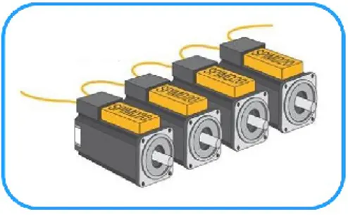
An example of power electronics device for distributed control is represented by the SPIMD20 of STMicroelectronics.
Figure 6: distributed solution
SPIMD20 is an 2 kW integrated motor drive for decentralized control; it can be installed directly on the motor case [1].
With this module it is possible to obtain the following advantages:
- Minimizing cabling systems and installation cost; - Control panel optimization from rack to the equipment; - Flexibility of automation architecture;
SPIMD20 is a complete compact motor drive solution in a single, robust and reliable module, including full bridge IGBT inverter, control unit and communication interface based on real-time industrial Ethernet.
It is ideal for applications with high number of 3-phase Brushless motors and real-time constraints:
- Packaging machines; - Process machines; - Multi-axial controls; - Robotics.
1.4 Power Electronics for Robotics Application
As described in the previous paragraph, the development of power electronics has made many interesting scenarios, such as industrial robotics and mobile robotics, possible in Robotics application.
New families of inverter, for example, allow the use of decentralized control. Thanks to the small dimensions of new inverter, indeed, it is possible to move the controllers of a robot directly on its axes, with advantages in terms of cable costs and flexibility.
Decentralized control in industrial robotics needs the knowledge of the state of each link; this is possible by means multi-sensor data fusion techniques that fuse together measurements coming from different sensors such as accelerometers, gyroscopes and encoders.
Power electronics devices, like inverter, can be very useful also in mobile robotics application, such as the control of unmanned ground vehicles (UGV) or unmanned aerial vehicles. In order to control the movements of an UGV, inverters allow the transformation of the control commands into the appropriate signals for the motors. Therefore, it is very important to know the right position of the motors axes. By using multi-sensor data fusion techniques, is also possible to localize the UGV, as is described in the sixth chapter of this thesis.
2 Multi-sensor data fusion
2.1 Introduction
The knowledge of the state of a dynamic system like an industrial robot is necessary in order to understand its dynamic behavior and to solve many control problems.
Theoretically the dynamics of a linear system can be determined from a complete knowledge of its mathematical model.
The discrete-time model of a linear system is:
𝒙𝒌 = 𝑨 𝒙𝒌−𝟏+ 𝑩 𝒖𝒌 (𝟏)
Where 𝑥𝑘 ∈ ℜ𝑛 is the state vector of the system at the current step k , xk-1 is
the state of the system at the previous step k-1, 𝑢𝑘 ∈ ℜ𝑙is the input of the system, 𝐴 ∈ ℜ𝑛𝑥𝑛is the state matrix that relates the state at the previous time step to the state at the current step, 𝐵 ∈ ℜ𝑛𝑥𝑙is the output matrix that relates the optional control input u to the state x.
However, unfortunately, the model of the system often is not enough accurate and is subject to the process noise w.
𝒙𝒌= 𝑨 𝒙𝒌−𝟏+ 𝑩 𝒖𝒌+ 𝒘𝒌−𝟏 (𝟐)
Another way to determine the state of the system could be by knowing the relation between the sensor measurements 𝑧𝑘 ∈ ℜ𝑚 and the state:
𝒛𝒌= 𝑯 𝒙𝒌 (𝟑)
Where the matrix 𝐻 ∈ ℜ𝑚𝑥𝑛 relates the state 𝑥
But usually the sensor measurements are noisy and the relation with the state is inaccurate:
𝒛𝒌= 𝑯 𝒙𝒌+ 𝒗𝒌 (𝟒)
where v is the measurement noise.
Multi-sensor data fusion:
allows to overcome these problems in order to get a better estimation of the state of the system, indeed it permits to exploit the advantages and to compensate the disadvantages of different sensors. is the process of combining observations from a number of different sensors to provide a robust and complete description of an environment or process of interest.
finds wide application in many areas of robotics such as object recognition, environment mapping, and localization.
method based on the Recursive Bayesian Filtering techniques, allows to integrate measurements from inertial sensors with measurements from different kind of sensors.
Recursive Bayesian Filtering techniques, are widely used for estimating the state of a dynamic system, because allow to overcome problems caused by uncertainty and noise.
Given the state space model of a dynamic system, composed by the state transition function and the measurement function,
{𝒙𝒌 = 𝒇( 𝒙𝒌−𝟏, 𝒖𝒌, 𝒘𝒌−𝟏) (𝟓) 𝒛𝒌 = 𝒉( 𝒙𝒌, 𝒗𝒌) (𝟔)
where f and h can be both linear or non-linear, the goal of the Recursive Bayesian Filtering is to estimate the evolution of the system state using all the measurements collected until the current time [2].
As the state of the system is a random variable, all the information about the state provided by the measurements are contained in the posterior probability density function (pdf) p(x), therefore the Recursive Bayesian Filtering has to provide an estimation of the posterior pdf.
𝒑(𝒙) = 𝒑(𝒙𝟎:𝒌|𝒛𝟏:𝒌) (𝟕)
Figure 8: Steps of Recursive Bayesian filter
2.2 The Kalman Filter
In the case in which both the transition and the measurement functions are linear and either the process and the measurement noise are Gaussian and additive, the optimal solution is given by the Kalman Filter (KF) [3].
The Kalman filter is essentially a set of mathematical equations that implement a predictor-corrector type estimator that is optimal in the sense that it minimizes the estimated error covariance when the previously cited conditions are met [3].
Given the linear dynamic state-space model of a system:
{𝒙𝒌 = 𝑨 𝒙𝒌−𝟏+ 𝑩 𝒖𝒌+ 𝒘𝒌−𝟏 (𝟖) 𝒛𝒌 = 𝑯 𝒙𝒌+ 𝒗𝒌 (𝟗)
where the process and measurement noise wk and vk have a normal probability
distributions:
𝒑(𝒘)~𝑵(𝟎, 𝑸) (𝟏𝟎) 𝒑(𝒗)~𝑵(𝟎, 𝑹) (𝟏𝟏)
the Kalman filter provides an a posteriori state estimate 𝒙̂𝒌 as a linear combination of an a priori estimate 𝒙̂𝒌− and a weighted difference between an actual measurement 𝒛𝒌 and a measurement prediction 𝑯 𝒙̂𝒌−:
𝒙
̂𝒌 = 𝒙̂𝒌−+ 𝑲
𝒌(𝒛𝒌− 𝑯 𝒙̂𝒌−) (𝟏𝟐) The difference (𝒛𝒌− 𝑯 𝒙̂𝒌−) in equation 12 is called measurement innovation, or
residual. The residual reflects the discrepancy between the predicted and the actual
measurements . A residual of zero means that the two are in complete agreement.
𝑲𝒌 is the Kalman gain or blending factor that minimizes the covariance 𝑷𝒌 of the posteriori error 𝒆𝒌 :
𝑷𝒌= 𝑬[𝒆𝒌𝒆𝒌𝑻] (𝟏𝟑) 𝒆𝒌 = 𝒙𝒌− 𝒙̂𝒌 (𝟏𝟒)
One form of K that minimizes the posteriori error covariance is given by:
𝑲𝒌 = 𝑷𝒌−𝑯𝑻(𝑯𝑷𝒌−𝑯𝑻+ 𝑹)−𝟏 (𝟏𝟓)
Table 1
Initial estimates for 𝒙̂𝒌−𝟏and 𝑷𝒌−𝟏 Time Update (“Predict”)
Project the state ahead 𝒙̂𝒌−= 𝑨 𝒙̂𝒌−𝟏+ 𝑩 𝒖𝒌 Project the error covariance ahead 𝑷𝒌−= 𝑨𝑷𝒌−𝟏𝑨𝑻+ 𝑸
Measurement Update (“Correct”)
Compute the Kalman gain 𝑲𝒌 = 𝑷𝒌−𝑯𝑻(𝑯𝑷𝒌−𝑯𝑻+ 𝑹)−𝟏 Update estimate with measurement zk 𝒙̂𝒌 = 𝒙̂𝒌−+ 𝑲𝒌(𝒛𝒌− 𝑯 𝒙̂𝒌−) Update the error covariance 𝑷𝒌= (𝑰 − 𝑲𝒌𝑯) 𝑷𝒌−
2.3 The Extended Kalman Filter
In the real world, the previously mentioned hypotheses are rarely encountered and therefore you have to cope with nonlinearities.
Generally, for nonlinear filtering, no exact optimal solutions can be obtained, however, under the assumption that the process and the measurement noise are Gaussian and additive, a classical method to solve the nonlinear filtering problem is the Extended Kalman Filter (EKF). In the EKF a linearization around the current estimate is applied to the system and the conventional Kalman filtering technique is further employed.
Let us consider a process governed by the non-linear equations:
{𝒙𝒌= 𝒇( 𝒙𝒌−𝟏, 𝒖𝒌, 𝒘𝒌−𝟏) (𝟏𝟔) 𝒛𝒌 = 𝒉( 𝒙𝒌, 𝒗𝒌) (𝟏𝟕)
with f and h non-linear functions, to estimate the state we need first to linearize the system around the current estimate by means of the following Jacobians [3]:
𝑊[𝑖,𝑗]= 𝜕𝑓[𝑖] 𝜕𝑤[𝑗] (𝑥̂𝑘, 𝑢𝑘, 0) (𝟏𝟕) 𝐴[𝑖,𝑗]= 𝜕𝑓[𝑖] 𝜕𝑥[𝑗](𝑥̂𝑘, 𝑢𝑘, 0) (𝟏𝟖) 𝐻[𝑖,𝑗] = 𝜕ℎ[𝑖] 𝜕𝑥[𝑗](𝑥̂𝑘, 0) (𝟏𝟗) 𝑉[𝑖,𝑗] = 𝜕ℎ[𝑖] 𝜕𝑣[𝑗](𝑥̂𝑘, 0) (𝟐𝟎)
Finally, the equations of the extended Kalman filter are:
Table 2
Initial estimates for 𝒙̂𝒌−𝟏and 𝑷𝒌−𝟏 Time Update (“Predict”)
Project the state ahead 𝒙̂𝒌−= 𝒇(𝒙̂
𝒌−𝟏, 𝒖𝒌, 0) Project the error covariance ahead 𝑷𝒌−= 𝑨
𝒌𝑷𝒌−𝟏𝑨𝒌𝑻+ 𝑾𝒌𝑸𝒌−𝟏𝑾𝒌𝑻 Measurement Update (“Correct”)
Compute the Kalman gain 𝑲𝒌= 𝑷𝒌−𝑯𝑻(𝑯𝑷𝒌−𝑯𝑻+ 𝑽𝒌𝑹𝒌−𝟏𝑽𝒌𝑻)−𝟏 Update estimate with measurement zk 𝒙̂𝒌= 𝒙̂𝒌−+ 𝑲𝒌(𝒛𝒌− 𝒉( 𝒙̂𝒌−, 𝟎)) Update the error covariance 𝑷𝒌= (𝑰 − 𝑲𝒌𝑯) 𝑷𝒌−
2.4 Particle Filter
Because EKF always approximates the posterior pdf as a Gaussian, it works well for some types of nonlinear problems, but it may provide a poor performance in some cases when the true posterior pdf is non-Gaussian (e.g. heavily skewed or multi-modal).
When the model is highly nonlinear or the noise is non-Gaussian, KF and its variants are no longer suited for estimating the state of a dynamic system.
The alternative to the Gaussian filters to which KF belong, is represented by the nonparametric filters.
The main difference between Gaussian filters and nonparametric filters is the different representation of the posterior pdf. The first class represents this pdf with a fixed function, the Gaussian function, while, on the other hand, the nonparametric filters represents the posterior pdf through a finite number of values, each of which roughly corresponds to a portion of the state space.
Among the nonparametric filters, the PF represent the posterior pdf through a high number of samples or particles. The aim of PF, as the Recursive Bayesian
Filtering technique, is to estimate the posterior pdf but, since it is generally
impossible to sample from it, the Monte Carlo Importance Sampling method is used [4]. The key idea of the Monte Carlo Importance Sampling method is to generate samples from a different pdf with particular characteristics called importance function instead of sampling from the posterior pdf directly and for each generated sample use a weighting factor to account for the mismatch between functions.
Therefore, ultimately the PF represents the required posterior pdf by a set of random samples or particles, generated as aforementioned, with associated weights.
In order to avoid the divergence of the estimation, a resampling step is executed by replicating the samples with high importance weights and removing samples with low weights.
Let us consider a process governed by the non-linear equations:
{𝒙𝒌 = 𝒇( 𝒙𝒌−𝟏, 𝒖𝒌, 𝒘𝒌−𝟏) (𝟐𝟏) 𝒛𝒌 = 𝒉( 𝒙𝒌, 𝒗𝒌) (𝟐𝟐)
Table 3 𝑓𝑜𝑟 𝑖 = 1: 𝑁𝑠 𝑥𝑘 𝑖 ~𝑞(𝑥𝑘|𝑥𝑘−1 𝑖 , 𝑧𝑘) = 𝑝(𝑥𝑘|𝑥𝑘−1 𝑖 ) 𝑤𝑘 𝑖 = 𝑤𝑘−1 𝑖 𝑝𝑣(𝑧𝑘|𝑥𝑘𝑖) End for 𝑁𝑜𝑟𝑚𝑎𝑙𝑖𝑧𝑒 𝑤𝑒𝑖𝑔ℎ𝑡𝑠 𝑅𝑒𝑠𝑎𝑚𝑝𝑙𝑒 𝒙 ̂𝒌 = 𝒙̂𝒌−𝟏+ ∑ 𝑤𝑘 𝑖 𝑁𝑠 𝑖=1 𝑥𝑘 𝑖
A comparison between the equations of the extended Kalman filter and the equations of the particle filter is shown in the following figure:
3 Inertial Sensors
3.1 Introduction
Inertial sensors are particular sensors that exploit the inertia of a mass contained inside them, to measure angular rates (gyroscopes) or linear accelerations (accelerometers).
In recent years the performances of MEMS inertial sensors have improved and their cost has decreased and thus they have been used successfully in many applications such as virtual reality, autonomous vehicle navigation and robotics.
As described in the following pages of this chapter, the accelerometers and gyroscopes measures are not sufficient for those applications where is necessary to have complete information about the attitude and the orientation of a rigid body like a robot.
In this chapter, indeed, the magnetometers are described as well.
Moreover, in addition to the main features and the principles of operation, for each sensor a calibration procedure is described.
For the calibration of the inertial sensors, a Kuka robot manipulator was used as a precision instrument to move the gyroscopes at known angular velocities and to let accelerometers assume known orientations.
3.2 Gyroscopes
The first gyroscope was a mechanical device (Fig.10) composed by a rotor and a Cardan suspension (gimbal) that, due to the law of conservation of angular momentum, when the rotor rotates at a fixed angular velocity, tends to maintain its rotation axis (spin axis) oriented in a fixed direction.
Figure 10: gyroscope
Each torque applied to the spin axis, due to the rotation of the gyroscope frame, causes a momentum orthogonal to the torque. The measure of the action of a servomotor that maintains the spin axes parallel to itself, provides the measure of the angular velocity of the initial rotation.
Today in precise application the optical gyroscopes are widely diffused and in particular the optical fiber gyroscopes that have high precision, are very simple and are not expensive since not require high precision mechanical parts.
Inexpensive vibrating structure gyroscopes manufactured with MEMS technology have become widely available. Internally, MEMS gyroscopes use lithographically constructed versions of one or more of the following mechanisms: piezoelectric, tuning forks, vibrating wheels, or resonant solids of various designs. MEMS gyroscopes are used in automotive roll-over prevention and airbag systems, image stabilization, and have many other potential applications.
The angular velocity measured by a gyroscope ωm [rad/sec] differs from the
expected one ω, due to the not unitary scale factors s, the constant component of the bias b and a random process n(t) that models the noise and the variable component of the bias.
𝝎𝒎 = 𝒔𝝎 + 𝒃 + 𝒏(𝒕) (𝟐𝟑)
The performance of the different types of gyroscopes are usually described by the stability of the bias and by the stability of the scale factor.
Nowadays gyroscopes are mainly used to get the angular velocity and the orientation in applications such as compasses, aircraft, mobile robots, computer pointing devices, consumer electronics, etc.
By integrating, with a processing unit, the angular velocity measured by a gyroscope, it is possible to get the tilt angle of the device.
Therefore, in addition to the angular velocity, gyroscopes allow to get information about the orientation of an object like for example an aircraft (fig.11):
However the integration of the measured angular velocity causes an accumulation of the noise over time that brings to the drift problem.
To contrast the drift problem of the gyroscopes measurements integration, it can be occasionally subtracted from the measurement or, as in this work is explained, it is possible to use a multi-sensor fusion method.
3.2.1 CALIBRATION
To convert the gyroscope's raw measurements to meaningful angular velocities a calibration procedure could be necessary, in particular for highly sensitive applications [5].
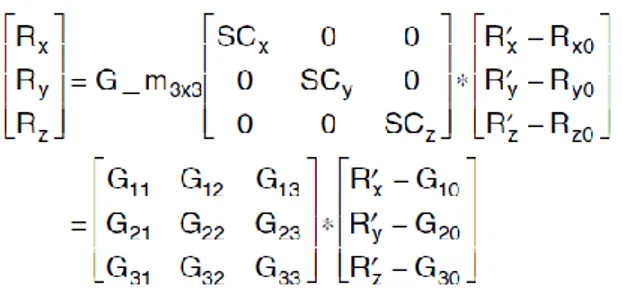
Considering a triaxial gyroscope, the relationship between the raw measurements and the meaningful angular velocity, can be written in the following way:
Figure 12: relationship between raw and calibrated measures
Where Rx, Ry, Rz are the calibrated angular velocity of each axis, G_m is the misalignment matrix between the gyro sensing axes and the device body axes,
SCx, SCy, SCz are the scale factors caused by the mismatch of the sensitivity of
each axis, Rx’, Ry’, Rz’ are the raw measurement of the gyroscope and Rx0, Ry0, Rz0 are the zero-rate level or bias for each axis.
One possible calibration procedure consists in the calculation of 12 parameters (G11…G30) by means of the least square method.
In particular the steps of the procedure are:
- Measure the zero-rate level Rx0, Ry0, Rz0 of each axis;
- Rotate the board around each axis at different known angular velocity and collect the measurements;
- Construct the known applied angular velocity matrix (Y); - Construct the gyroscope’s raw measurements matrix (w);
- Apply the Least Squares method to determine the 12 calibration parameters (X);
𝐘 = 𝐰 ∙ 𝐗 𝐗 = [𝐰𝐓𝐰]−𝟏𝐰𝐓𝐘 (𝟐𝟒)
3.3 Accelerometers
An accelerometer is a device that measures linear accelerations.
Conceptually, an accelerometer behaves as a damped mass on a spring; it is composed of a mass m constrained to two guides that can move only along a specific direction. The mass is also connected to the frame by a spring (with stiffness k) that acts parallel to the guides.
By measuring the displacement of the mass it is possible to get the acceleration to which the mass is subjected.
Figure 13: scheme of an accelerometer
Similarly to the case of the gyroscopes, the acceleration am [m/s^2] measured
by an accelerometer differs from the expected one, due to the not unitary scale factor, the constant component of the bias b and due to a random process n(t) that models the noise and the variable component of the bias.
𝒂𝒎= 𝒔𝒂 + 𝒃 + 𝒏(𝒕) (𝟐𝟓)
The various types of accelerometers can differ for the materials used, manufacturing technology, principle of operation (pendulum, quartz resonant, floated mechanical), the operating range, bandwidth, etc.
Therefore important performance parameters are the stability of the bias and the stability of the scale factor.
Accelerometers can be heavily miniaturized and represent the reference product for the MEMS industries.
3.3.1 STATIC CONDITIONS
The accelerometers, in static conditions, are sensitive only to the acceleration of gravity g, and then can be used to partially reconstruct the orientation of a body [6].
Figure 14: pitch angle
𝐑𝐎𝐋𝐋 𝐀𝐍𝐆𝐋𝐄 𝜸 = 𝒂𝒕𝒂𝒏𝟐(𝑨𝒚, 𝑨𝒛) (𝟐𝟔) 𝐏𝐈𝐓𝐂𝐇 𝐀𝐍𝐆𝐋𝐄 𝜽 = 𝒂𝒕𝒂𝒏𝟐(𝑨𝒙, 𝑨𝒛) (𝟐𝟕)
Where 𝐴𝑥, 𝐴𝑦, 𝐴𝑧 are the components of gravity vector, that are measured in static conditions.
The reconstruction of the attitude of a body is partial because accelerometers are insensitive to rotations about an axis parallel to the vector g.
Figure 15: heading angle
For this reason, in many applications, where it is necessary reconstruct the complete orientation of a body, magnetometers are used as well.
3.3.2 DYNAMIC CONDITIONS
In dynamic conditions accelerometers sense also the external inertial accelerations to which it is subjected:
For movements on linear paths, accelerometers in addition to gravity detect the component of the linear acceleration too:
Figure 16: linear path
For movements on curved paths, accelerometers detect centripetal (acp) and
tangential acceleration (at) in addition to gravity:
Figure 17: curved path
Nowadays, accelerometers are also used to help the GNSS (Global Navigation Satellite Systems) as the GPS to evaluate the speed or the position of an object when a satellite signal is not available, for example inside buildings or in tunnels. However, the speed provided by the accelerometer is increasingly unreliable over time due to the drift of integration and to the noise.
𝑎(𝑡) =𝑑𝑣(𝑡) 𝑑𝑡 = 𝑑2𝑝(𝑡) 𝑑𝑡2 (𝟐𝟗) 𝑣(𝑡) = 𝑣0+ ∫ 𝑎(𝑡)𝑑𝑡 𝑡 𝑡0 (𝟑𝟎) 𝑝(𝑡) = 𝑝0+ 𝑣0(𝑡 − 𝑡0) + ∫ ∫ 𝑎(𝑡)𝑑𝑡 𝑡 𝑡0 (𝟑𝟏) 3.3.3 CALIBRATION
To convert the accelerometer’s raw data to meaningful angular accelerations, a calibration procedure could be necessary, in particular for highly sensitive applications [6].
Considering a tri-axial accelerometer, the relationship between the raw measurements and the meaningful acceleration, can be written in the following way:
Figure 18: relationship between raw and calibrated measures
Ax1, Ay1, Az1 are the normalized acceleration of each axis;
A_m is the misalignment matrix between the accelerometer sensing axes and
the device body axes;
A_SCx, A_SCy, A_SCz are the scale factors of each axis that represent the
mismatch of the sensitivity;
Ax, Ay, Az are the accelerometer raw measurements of each axis; A_OSx, A_OSy, A_Osz are the offsets of each axis;
The previously relation can be rewritten in the following way:
Figure 19: matrix form of the relationship
One possible calibration procedure consists in the calculation of 12 parameters (ACC11…ACC30) by means of the least square method.
In particular the steps of the procedure are:
1. Collect accelerometer raw data at 6 known stationary positions; 2. Construct the matrix of sensor raw data (w);
3. Construct the known earth gravity vector (Y);
4. Then apply the Least Squares method to determine the 12 calibration parameters (X);
3.4 Magnetometers
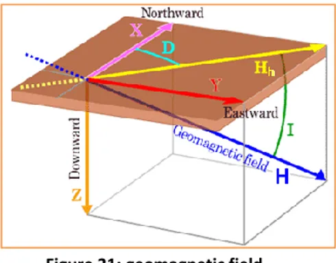
Magnetometers are measurement instruments that measure magnetic fields such as the geomagnetic field.
Local earth magnetic field H has a component Hh(Xh,Yh) on the horizontal plane pointing to the earth’s magnetic north.
Figure 20: magnetic and geographic poles
Figure 21: geomagnetic field
As it is possible to notice in the figures 19 and 20, magnetic poles are not aligned with the Geographic poles, and the angle D takes into account this misalignment.
The projection of the geomagnetic field on the 3 axes allows the heading angle to be computed.
Heading is defined as the angle between the X axis (northward) and
Hh(Xh,Yh) [6].
YAW ANGLE = 𝒂𝒓𝒄𝒕𝒂𝒏 (𝒀𝒉
𝑿𝒉) (𝟑𝟑)
Figure 18: heading angle
In order to get correct heading information from the magnetic measurements, it is necessary to consider two different cases:
1. Leveled position:
If Roll and Pitch angles are both equal to zero, no compensation is necessary and Xh and Yh are equal to the magnetic measurements.
2. Tilted position:
If Roll and/or Pitch angles are not equal to zero, a tilt compensation is necessary.
Xh = Xmcos(Pitch) + Zmsin(Pitch) (34) Yh = Xmsin(Roll)sin(Pitch) + Ymcos(Roll)- Zmsin(Roll)cos(Pitch) (35)
Where pitch and roll angle can be computed using the accelerometer measurements.
3.4.1 CALIBRATION
To convert the magnetometer’s raw data to a meaningful magnetic information a calibration procedure could be necessary, in particular for highly sensitive applications [6].
Considering a tri-axial magnetometer, the relationship between the raw measurements and the meaningful acceleration can be written in the following way:
Figure 19: relationship between raw and calibrated measures
where Mx1, My1 and Mz1 are the normalized magnetic measurements of each axis, M_m is the misalignment matrix between the magnetic sensor sensing axes and the device body axes, M_SCx, M_SCy and M_SCz are the scale factors of each axis (mismatch of the sensitivity of the sensor sensing axes), M_si is the alignment matrix to compensate the soft-iron distortion, Mx, My and Mz are the
magnetometer raw measurements of each axis, M_OSx, M_OSy and M_Osz are the offsets of each axis caused by hard-iron distortion [6].
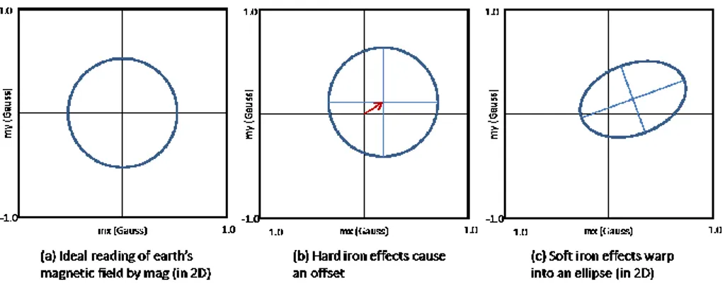
Hard-iron interference magnetic field is normally generated by ferromagnetic materials with permanent magnetic fields that are part of the handheld device structure. These materials could be permanent magnets or magnetized iron or steel. They are time invariant. These unwanted magnetic fields are superimposed on the output of the magnetic sensor measurements of the earth's magnetic field. The effect of this superposition is to bias the magnetic sensor outputs.
A soft-iron interference magnetic field is generated by the items inside the handheld device [6]. They could be current carrying traces on the PCB or magnetically soft materials. They generate a time varying magnetic field that is superimposed on the magnetic sensor output in response to the earth's magnetic field. The effect of the soft-iron distortion is to make a full round rotation circle become a tilted ellipse.
Figure 20: hard and soft iron distortions
Without hard-iron and soft-iron distortions the magnetic measures should be in a sphere of radius equal to the earth’s magnetic field strength, but actually they draw a tilt ellipsoid which can be described by the following equation:
Figure 21: magnetic measures ellipsoid equation
where x0, y0 and z0 are the offsets M_OSi (i = x, y, z) caused by hard-iron distortion, x, y and z are the magnetic sensor raw data Mx, My and Mz, a, b and c are the semi-axes lengths, d, e and f are the cross axis effect to make the ellipsoid tilted, R is the earth’s magnetic field strength.
If there is no soft-iron distortion inside the device, or the soft-iron effect is very small and can be ignored:
Figure 22: simplified ellipsoid equation
Therefore, the least square fitting ellipsoid method can be used to discover the parameters of M_SCi, M_OSi (i = x, y, z) and [M_si].
Let's assume there is no soft-iron distortion. The soft-iron matrix [M_si] is a 3x3 identity matrix. Then above equation can be rewritten as:
After three full round rotations magnetic sensor raw data have been collected, it is possible to combine Mx, My, and Mz as column vector and row vector. Then the above equation becomes:
The least square method can be applied to determine the parameters X vector as:
Then,
Let,
Then obtain:
Let,
Then,
The scale factor M_SCi (i = x, y, z), the offset caused by hard-iron distortion
M_OSi, and the 3x3 matrix [M_si] caused by soft-iron distortion have been
determined. Applying these parameters to the measurements of the rotations, we obtain a centered unit sphere.
Similarly, the least square method can be used to determine the [M_si] 3x3 matrix when there is soft-iron distortion.
4 Industrial Robotics
4.1 Introduction
Current efforts of research activity in Industrial Robotics are mainly focused on improving the performance of the robot, reducing the cost, improving the safety, introducing new features (plug and play , modularity, redundancy, human robot interaction) [7][8].
Nowadays the most common sensors to measure the joints angles of an industrial manipulator are the encoders. Through the joints angles by using kinematic equations you can get the position and the orientation of every link of the manipulator.
High precision and accuracy are necessary in many robotics applications such as manufacturing [8][9], welding [9], and increasingly medical applications [10].
The encoders, in particular the high resolution ones, have the advantage of being very accurate, but unfortunately they suffer of some weaknesses such as the high cost and the need of a tight mechanical coupling [11] with the motor shaft.
Therefore, measurements from the encoders of the robot joints do not always suffice to provide the accurate position of the joints, since the motor angle does not exactly coincide with the joint angle, due to gear backlash and joint flexibility.
MEMS Inertial sensors overcome these problems since they are low cost and do not need mechanical coupling; thus, they can represent another way to measure the joints angles of an industrial manipulator.
The aim of this work is to estimate the joints angles of a 6-DOF manipulator by integrating inertial sensors measurements by means of Recursive Bayesian Filtering techniques such as the Kalman Filter (KF) and the Particle Filter (PF).
A brief state of the art of the use of inertial sensors in the estimation of joint angle is now presented.
Regarding to the use of the MEMS inertial sensors to measure the joints angles of a robotic arm, some methods with different configuration of sensors based on the rigid-body kinematics are analyzed in [12]. Experimental results show that after calibration, it is possible to get good estimation of joints angles and angular rates.
MEMS inertial sensors need a calibration procedure to ensure meaningful measurements. Two calibration procedures are described in [11]. The proposed techniques allow detecting the joint angles of a mini-excavator that works in harsh working environment, by using accelerometers.
Low cost MEMS inertial sensors can be even used in combination with low resolution encoders in order to exploit the advantages and to compensate the disadvantages of both and eventually, obtain a sensor fusion approach as proposed in [13], to estimate angle and angular rate.
In order to get good and reliable results in the estimation of the joints angles of a manipulator, it is essential to know both the mounting position and the orientation of the sensors; a method to estimate the orientation and the mounting position of the accelerometer on the robot is proposed in [14].
In [15] measurements from an optical sensor and inertial sensors are fused together by means of a KF to estimate the end effector position.
In [16] there are some experiments of applying of the EKF to estimate the joints angles of a robotic manipulator by using low-cost MEMS accelerometer in order to control the manipulator. Two calibration accelerometer approaches are illustrated.
In [17] another useful application of the PFs which allow to estimate position and orientation of an object using a position sensor and an inertial measurement unit is shown. In this paper, a PF is used to estimate the orientation and a KF is used to estimate the position and the velocity. The presented experimental results show that this hybrid method is able to find a good estimation of the orientation
even when the initial orientation is completely unknown. Moreover, factors like number of particles and position sensor noise are demonstrated to affect the orientation error.
Recursive Bayesian Filtering based on inertial sensors have been used to track the movements of the human hand and control a robot manipulator in [18].
There are not many publications regarding the application of the PF to industrial robotics. Nevertheless it is very interesting to investigate on this topic, because PFs can offer many advantages compared to the EKF.
In [19] a PF is used to estimate the joints positions and the joints angular velocities of three DOF industrial robot, using measurements that come from an accelerometer, mounted on the end effector of the robotic manipulator, and from the encoders of the joints motors. In addition, the dynamic model of the robot is used and no process noise is considered, moreover a comparison with the EKF is performed.
An efficient approach that incorporates the Kalman filter (KF) and particle filter (PF) to estimate the position and orientation of the manipulator is proposed in [20].
The angle, the angular velocity and the angular acceleration of the first three joints of a 6 DOF robot are instead estimated in the works [21] and [22] using both a PF and an EKF, still through information from an accelerometer on the tool and motor angle measurements. In this case, a laser positioning system is also used to evaluate the performance. In the case of the EKF a Gaussian distribution of the noise is assumed, and a linearization only in the measurement relation is performed.
In order to obtain a high accuracy for positioning and orientation of the end-effector of industrial robots, in [23] the PF and the EKF are compared with the results indirectly obtained by a PD controller. Starting from the differential equation of a dynamic model of a two-link flexible manipulator and using Gamma noise (non-Gaussian) as both system noise and observation noise, the results show that PF and EKF have better performance (lower error variances) than PD controllers.
Similarly, in [24] the PF and the EKF are applied to a standard industrial manipulator as sensor fusion techniques and, moreover, the Cramer Rao Lower Bound is used to evaluate the performance of the angular position estimation.
Also in this case motor angle measurements and accelerometer measurements are used in the filters and the result is evaluated with respect to the tracking performance and in terms of position accuracy of the tool.
Measurements from a 3-axis gyroscope mounted on the end-effector is also used in [25] for estimating the end-effector position. A double weighting system is used to weigh the fusion of the sensors measurements and then to evaluate the particle weight for each sensor. Experiments are performed on a 3-DOF robotic manipulator and the results show that the approach improves the position estimate accuracy.
A method to estimate joints angles of a manipulator arm using one MEMS accelerometer and gyroscope pair instead of one optical encoder for each link is presented in [26].
In this work the kinematic model of the manipulator has been used and, unlike most of the cited works, in the methods proposed in this work, the encoders have not been used.
4.2 Model of the Manipulator
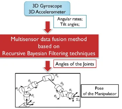
The aim of this work is to estimate the joints angles of an anthropomorphic manipulator using inertial sensors measurements combined together by means of a new Recursive Bayesian Filtering based multi-sensor fusion method.
Figure 28: pose estimation scheme
In particular both KF and PF have been used. In order to use both KF and PF, the knowledge of the model of the anthropomorphic manipulator is needed.
The robot can be considered as a multi-body system, composed by 6 joints and the angle of each single joint is considered as state variable.
Regarding to the use of the sensors measurements into the model equations, for each joint, the gyroscope measurements have been used in the transition equation to obtain the derivative of the joint angles, while the accelerometer measurements have been used in the measurements equation.
The equations of the dynamic state-space model that characterize the manipulator are the following:
{𝒒𝒋(𝒌 + 𝟏) = 𝒒𝒋(𝒌) + ∆𝒕 ∗ 𝒒̇𝒋(𝒌) + 𝒓𝒌−𝟏 (𝟑𝟔) 𝒈𝒋= 𝑹𝟎 𝒋 ∗ 𝒈𝟎+ 𝒗𝒌 (𝟑𝟕)
Where g0, gj are the accelerations of gravity expressed in the base reference
system of the manipulator and in the reference system of the j-th joint respectively, while 𝑅0 𝑗 is the rotation matrix between the base reference system and the reference system of the j-th joint.
All the reference systems have been chosen according to the Denavit-Hartenberg convention (Fig. 31) that is the standard approach [27].
Figure 29: reference systems
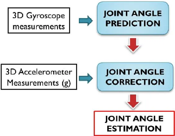
The proposed multi-sensor fusion method is based on Recursive Bayesian Filtering, and it is composed by two main steps, prediction and correction. In particular gyroscopes measurements are used for the prediction step in the state transition equation while the accelerometers measurements in the measurement function for the correction of the estimation.
The state transition equation is obtained by discretizing the time, with sampling step Δt, and approximating the derivative of the joint angle with the Euler method for numerical integration:
𝒒𝒋(𝒌 + 𝟏) = 𝒒𝒋(𝒌) + ∆𝒕 𝒒̇𝒋(𝒌) (𝟑𝟖)
The derivative of the joint angle 𝑞̇𝑗 is obtained using the gyroscopes measurements ω with the following relation:
{𝝎𝒋}(𝟎)= {𝝎𝒋−𝟏}(𝟎)+ 𝒒̇𝒋{𝒉𝒋−𝟏}(𝟎) (𝟑𝟗)
Where {ωj}(0) is the angular velocity of the j-th arm expressed in the base
reference system of the manipulator and hj-1 is the rotation versor of the j-th arm
joint.
In this relation the angular velocity {ωj}(0) of the j-th arm is expressed in the
base reference system of the manipulator, however we are interested in evaluating the angular velocity in the reference system of the joint, therefore the following transformation for the j-th joint should be applied:
𝝎𝒋(𝒋)= 𝑹𝟎𝒋 ∗ 𝝎𝒋(𝟎) (𝟒𝟎)
By substituting:
𝝎𝒋(𝒋)= 𝑹𝟎𝒋 ∗ {𝝎𝒋−𝟏}(𝟎)+ 𝒒̇𝒋∗ 𝑹𝟎 𝒋
∗ {𝒉𝒋−𝟏}(𝟎) (𝟒𝟏)
Finally, the state transition equation is:
𝒒̇𝒋= (𝑹𝟎 𝒋
∗ 𝒉𝒋−𝟏) †
𝒒𝒋(𝒌 + 𝟏) = 𝒒𝒋(𝒌) + ∆𝒕 ∗ (𝑹𝟎 𝒋
∗ 𝒉𝒋−𝟏) †
∗ (𝝎𝒋(𝒋)− 𝑹𝟎𝒋𝝎𝒋−𝟏(𝟎)) + 𝒓𝒌 (𝟒𝟑)
Where the symbol † indicate the pseudoinverse (left inverse in this case) matrix, that is the generalization of the inverse matrix for the case in which the matrix is not a square matrix .
Both 𝑅0 𝑗 and hj-1 depends on the state at the previous step qj(k), hence,
considering the angular velocities as input, the relation between the current state and the state at previous step is nonlinear and the process noise is additive.
The prediction of the angle is obtained by integrating the gyroscopes measurements, but it carries to the drift problem.
The drift of the estimation is because of the accumulation of the white noise of the reading in the integration.
To contrast the drift problem of the gyroscopes measurements integration, a new state variable, the bias, is introduced for each gyroscope.
The equations for the biases are slightly different for the EKF and for PF and will be presented in the next sections.
As regards the measurement function, during slow movements, the 3-axis accelerometer senses the components of the acceleration of gravity g expressed in the reference system of the j-th joint and therefore it is possible to exploit the acceleration of gravity in the base system as reference in order to obtain the joint angle:
𝒈𝒋= 𝑹𝟎 𝒋 ∗ 𝒈𝟎+ 𝒗𝒌 (𝟒𝟒)
In the measurement function, that is nonlinear, the rotation matrix 𝑅0 𝑗depends on the predicted state qj(k+1) , obtained at the previous step with the state transition equation, and, therefore, as it is possible to see in the previous equation, also the measurement function is nonlinear.
However, in our considered manipulator configuration, the axis of the first a joint is always parallel to the gravity acceleration vector, then in this case it is impossible to use the accelerometers measures to correct the estimation of the angle of the first joint.
Figure 24: joint estimation scheme
4.3 Methodology
Analyzing the structure of an anthropomorphic manipulator it is possible to notice that in order to reduce costs and to avoid redundancy, the minimum number of inertial platforms needed is three.
As it is possible to see in Fig. 31, the three inertial platforms are mounted on the 2nd, on the 4th, and on the 6th joint, respectively.
Figure 25: IMU boards
Figure 26: joint angles
With this choice it is possible to decouple the general estimation problem in three sub problems, hence three cascaded Filters may be considered (Fig. 35).
Figure 27: cascaded filters
Each Filter will estimate two joint angles, and in particular the first filter will estimate the angles of the first and the second joint, the second filter will estimate the angles of the third and the fourth joint and finally the third filter will estimate the angles of the fifth and sixth joint.
In addition, each filter will estimate the related three gyroscopes biases:
[𝒙𝒏] = [ 𝒒𝟐𝒏−𝟏 𝒒𝟐𝒏 𝒃𝒙_𝝎𝟐𝒏 𝒃𝒚_𝝎𝟐𝒏 𝒃𝒛_𝝎𝟐𝒏] (𝟒𝟓)
Therefore the equations of the derivative of joints angles become:
{𝒒̇𝟏(𝒌) 𝒒̇𝟐(𝒌)} = [ 𝐬𝐢𝐧 𝒒𝟐(𝒌) 𝟎 𝐜𝐨𝐬 𝒒𝟐(𝒌) 𝟎 𝟎 𝟏 ] † {𝝎𝟐}(𝟐) (𝟒𝟔)
{𝒒̇𝒒̇𝟑(𝒌) 𝟒(𝒌)} = [ 𝐬𝐢𝐧 𝒒𝟒(𝒌) 𝟎 𝟎 𝐜𝐨𝐬 𝒒𝟒(𝒌) −𝟏 𝟎 ] † ({𝝎𝟒}(𝟒)− 𝑹𝟐 𝟒{𝝎𝟐}(𝟐)) (𝟒𝟕) {𝒒̇𝒒̇𝟓(𝒌) 𝟔(𝒌)} = [ 𝐬𝐢𝐧 𝒒𝟔(𝒌) 𝟎 𝐜𝐨𝐬 𝒒𝟔(𝒌) 𝟎 𝟎 𝟏 ] † ({𝝎𝟔}(𝟔)− 𝑹𝟒 𝟔{𝝎𝟒}(𝟒)) (𝟒𝟖)
In the equations (47) and (48) it is possible to notice that, in order to estimate the proper joint angles, for the second and the third filter it is necessary to subtract the gyroscopes measurements of the previous arms.
4.4 Kalman Filter
Since the equations of the model are nonlinear, the Extended version of the KF has been used in this work.
Prediction of the state is realized with the following equations:
{𝒙𝒌+𝟏|𝒌𝒏 } = [Ф]{𝒙𝒌𝒏} + [Г]{𝒙̇𝒌𝒏} + 𝒓𝒌 (𝟒𝟗) [𝑷𝒌+𝟏|𝒌𝒏 ] = [𝑨𝒌+𝟏|𝒌][𝑷𝒌𝒏][𝑨𝒌+𝟏|𝒌] 𝑻 + [𝑾𝒌+𝟏|𝒌][𝑸][𝑾𝒌+𝟏|𝒌] 𝑻 (𝟓𝟎) Where [Ф] = [1 0 0 1], [Г] = [ ∆t 0
0 ∆t] since ∆𝑡 is the sampling time of the filter and 𝑟𝑘 is the process noise.
𝑃𝑘+1|𝑘𝑛 is the matrix of the error covariance, the matrices 𝐴𝑘+1|𝑘 and 𝑊𝑘+1|𝑘 are the Jacobian of the state equations:
[𝐴𝑘+1|𝑘] = 𝜕𝑓(𝑥𝑘+1|𝑘𝑛 ) 𝜕𝑥 (51) [𝑊𝑘+1|𝑘] = 𝜕𝑓(𝑥𝑘+1|𝑘𝑛 ) 𝜕𝑟 (52)
and the matrix Q is the covariance matrix of the process noise r.
In the EKF the biases are supposed constant during the prediction phase and in each step they are added to the gyroscopes measurements.
Therefore, in the prediction phase, the predicted gyroscopes biases have been added to the gyroscopes measurements, before they are integrated:
{𝑏𝜔𝑗(𝑗)(𝑘 + 1)} = {𝑏𝜔𝑗(𝑗)(𝑘)} (53)
{𝜔𝑗(𝑗)(𝑘 + 1)} = {𝜔𝑗(𝑗)(𝑘 + 1)} + {𝑏𝜔𝑗(𝑗)(𝑘 + 1)} (54)
After the prediction step, accelerometers measurements are used to correct the state estimation; in the EKF the correction is obtained using the following equations: [𝐾𝑘+1𝑛 ] = [𝑃 𝑘+1|𝑘𝑛 ][𝐻𝑘+1|𝑘] 𝑇 ([𝐻𝑘+1|𝑘][𝑃𝑘+1|𝑘𝑛 ][𝐻𝑘+1|𝑘] 𝑇 + [𝑉𝑘+1|𝑘][𝑆][𝑉𝑘+1|𝑘] 𝑇 )−1 (55) {𝑥𝑘+1𝑛 } = {𝑥 𝑘+1|𝑘𝑛 } + [𝐾𝑘+1𝑛 ] ({𝑧𝑘+1𝑛 } − [𝑅({𝑥𝑘+1|𝑘𝑛 })]2𝑛−2 2𝑛 {𝑔𝑘+1}2𝑛−2) (56) [𝑃𝑘+1𝑛 ] = (𝐼 − [𝐾 𝑘+1𝑛 ][𝐻𝑘+1|𝑘])[𝑃𝑘+1|𝑘𝑛 ] (57)
Where 𝐾𝑘+1𝑛 is the Kalman gain, 𝐻𝑘+1|𝑘 and 𝑉𝑘+1|𝑘 are the Jacobian of the measurement equation and S is the covariance matrix of the accelerometers noise
v. [𝐻𝑘+1|𝑘] = 𝜕ℎ(𝑥𝑘+1|𝑘𝑛 ) 𝜕𝑥 (58) [𝑉𝑘+1|𝑘] = 𝜕ℎ(𝑥𝑘+1|𝑘𝑛 ) 𝜕𝑣 (59)
Both the Jacobian, related to the process noise and accelerometers noise respectively, are identity matrices, because the noises are additive.
For the second and the third filter, to be able to calculate the Jacobian (58) it is necessary to use the joint angles estimated by the previous filters.
Therefore, the second filter will have as inputs the gyroscopes measurements of the first board and the estimation of the first and the second joint angle; finally, the third filter will have as input the gyroscopes measurements of the second board and the estimation of the first, the second, the third and the fourth joint angles.
4.5 Particle Filter
In the PF, for each particle i, the prediction step is realized with the prior pdf:
𝑥𝑘 𝑖 ~𝑝(𝑥𝑘|𝑥𝑘−1 𝑖 ) = 𝑓( 𝑥𝑘−1, 𝑢𝑘) (60)
It is possible to notice that it consists of evaluating the state transition equation of the model of the manipulator, like for the EKF, many times as the particle number.
As regards the gyroscopes biases, they have been modelled through a Gaussian distribution, with the same standard deviation of the gyroscope
measurements and have been accumulated step by step; two non-linear weighting factors, the sine and cosine functions, have been used for the x and y components, to weigh more the bias of the axis involved in the rotation.
{𝑛𝑜𝑖𝑠𝑒−𝜔𝑗 𝑗 (𝑘)} = 𝑛𝑜𝑟𝑚𝑟𝑛𝑑 (0, 𝑠𝑡𝑑 {𝜔𝑗𝑗} ) (61) 𝑏𝜔𝑗𝑥(𝑗)(𝑘 + 1) = 𝑏𝜔𝑗𝑥(𝑗)(𝑘) + 𝑠𝑖𝑛(𝑞𝑘 𝑖 ) ∗ 𝑛𝑜𝑖𝑠𝑒−𝜔𝑗𝑥 𝑗 (𝑘) (62) 𝑏𝜔𝑗𝑦(𝑗)(𝑘 + 1) = 𝑏𝜔𝑗𝑦(𝑗)(𝑘) + 𝑐𝑜𝑠(𝑞𝑘 𝑖 ) ∗ 𝑛𝑜𝑖𝑠𝑒 −𝜔𝑗𝑦 𝑗(𝑘) (63) 𝑏𝜔𝑗𝑧(𝑗)(𝑘 + 1) = 𝑏𝜔𝑗𝑧(𝑗)(𝑘) + 𝑛𝑜𝑖𝑠𝑒−𝜔𝑗𝑧 𝑗(𝑘) (64) {𝜔𝑗(𝑗)(𝑘)} = {𝜔𝑗(𝑗)(𝑘 + 1)} + {𝑏𝜔𝑗(𝑗)(𝑘 + 1)} (65) Where {𝑛𝑜𝑖𝑠𝑒−𝜔𝑗
𝑗(𝑘)} is the Gaussian noise accumulated step by step, 𝑏𝜔 𝑗
(𝑗) is the gyroscopes bias and normrnd is the MATLAB function for Gaussian distribution.
In the PF, a weight is associated to each particle to give more importance to the best particles by means of the accelerometers measurements:
𝑤𝑘 𝑖 = 𝑤𝑘−1 𝑖 𝑝(𝑧𝑘|𝑥𝑘 𝑖 ) (66)
𝑤𝑘 𝑖 = 𝑤𝑘−1 𝑖 𝑝𝑣(𝑧𝑘− ℎ( 𝑥𝑘)) (67)
Where 𝑤𝑘 𝑖 is the particle weight index and 𝑝
𝑣 is the pdf of the accelerometers noise that in this case is Gaussian.
Even for the PFs, like the EKFs, the second filter needs the estimation of the first and the second joint angles, while, the third filter needs the estimation of the first, the second, the third and the fourth joint angles.
In order to avoid the divergence of the estimation, a resampling step is executed by replicating the samples with high importance weights and removing samples with low weights.
Finally the state estimation is:
𝑥̂𝑘 = 𝑥̂𝑘−1+ ∑ 𝑤𝑘 𝑖 ∗ 𝑃𝑎𝑟𝑡𝑖𝑐𝑙𝑒𝑠
𝑖=1
𝑥𝑘 𝑖 (68)
In both techniques the initialization of the state is performed by using the accelerometers measurements in static conditions, but in the EKF the initial state corresponds to the angle obtained from the accelerometers measurements while in the PF the particles are initialized with a Gaussian distribution centered in the angle obtained from the accelerometers measurements.
4.6 Experimental Setup
The robot used for the experiments is a KUKA KR 5 sixx R850 that is a six degrees-of-freedom anthropomorphic robot.
Figure 28: Kuka KR 5 sixx R850
The inertial platform used in this work is the MTi by Xsens that includes a triaxial accelerometer and a triaxial gyroscope.
In the experiments that have been conducted, the three IMUs mounted on the arms send the raw data to a PC for offline processing to get the estimation of the angles of the joints. The estimation of the state can be compared with the joint angles measured by the high-resolution encoders of the robot. In the first part of the experiments the robot is maintained in static conditions in order to initialize the state of the system and to compensate the offset of the gyroscopes.
4.7 Experimental Results
About fifty experimental tests have been performed to assess the real performance and limitations of the method.
The results of two tests are presented.
The sample time ∆t used for both filtering techniques is 0.012 s and the number of particles is 2000. The estimation of the joints angles obtained with the simple gyroscopes integration is also presented.
4.7.1 First Experiment
The first test is composed by single joint movements.
In order to evaluate the performance of the proposed methods, the encoders have been used as reference precision system.
Figure 29: joint angles
As it is possible to notice from the images below, in the first experiment, the first board has the best performance while the last one has the worst performance for both methods.
The error on the estimation of the angles of the two first joints is very low and is, in both methods, between +1° and -1°.
Figure 30: angle error on the first joint
Figure 31: : angle error on the second joint
As regard the estimation of the angles of the third and the fourth joint, the two methods have almost the same performances and the maximum error is for both almost 1.5°.
Figure 38: : angle error on the third joint
0 20 40 60 80 100 120 140 160 -1 -0.5 0 0.5 1 time [s] q 1 e rr [° ] EKF PF gyros 0 20 40 60 80 100 120 140 160 -1 -0.5 0 0.5 1 time [s] q 2 e rr [° ] EKF PF gyros 0 20 40 60 80 100 120 140 160 -2 -1 0 1 2 time [s] q 3 e rr [° ] EKF PF gyros
Figure 39: : angle error on the fourth joint
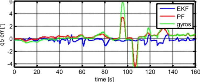
As it is easy to see in the tables 1,2 and 3 , the error in the estimation of the angles of the fifth and sixth joints is higher than that of the other joints, because the last board feels the inaccuracy of the previous estimations and because in the last joint there are more vibrations.
Figure 32: : angle error on the fifth joint
Figure 33: : angle error on the sixth joint
0 20 40 60 80 100 120 140 160 -2 -1 0 1 2 time [s] q 4 e rr [° ] EKF PF gyros 0 20 40 60 80 100 120 140 160 -4 -2 0 2 4 6 time [s] q 5 e rr [° ] EKF PF gyros 0 20 40 60 80 100 120 140 160 -4 -2 0 2 4 6 time [s] q 6 e rr [° ] EKF PF gyros
The maximum error in the fifth joint is about 4.5° with PF and about 1° with EKF, while in the sixth joint is almost 4° with EKF and almost 6° with PF.
In the estimation of the angles of the last two joints, the two methods have different performance and in particular the EKF has better performance than the PF because the EKF is able to compensate the noise caused by the vibrations.
Table 4: joints estimation error (EKF) [°]
joint mean standard deviation root mean square max 1 0.01 0.16 0.16 0.37 2 -0.08 0.11 0.13 0.66 3 0.22 0.20 0.30 1.22 4 -0.01 0.17 0.17 0.99 5 -0.21 0.27 0.35 1.16 6 0.25 0.85 0.89 3.91
Table 5: joints estimation error (PF) [°]
joint mean standard deviation root mean square max 1 -0.34 0.16 0.37 0.69 2 -0.06 0.13 0.14 0.59 3 0.18 0.54 0.57 1.39 4 -0.14 0.60 0.62 1.59 5 0.31 0.83 0.88 4.41 6 2.85 1.78 3.36 5.59
Table 6: joints estimation error (Gyros integration) [°]
joint mean standard deviation root mean square max 1 0.02 0.16 0.16 0.37 2 0.39 0.20 0.44 0.90 3 -1.04 0.65 1.23 2.02 4 0.11 0.28 0.30 0.99 5 0.23 1.38 1.40 7.11 6 4.72 3.20 5.71 10.58
In order to understand if the proposed methods are valid alternatives to the classic encoder, is important to analyze the performance in positioning of the end effector.
The position of the end-effector of the manipulator is shown in the following figure:
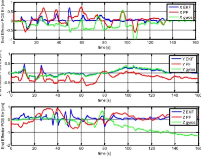
Figure 35: end effector position error
Although each joint angle estimation has a small error, these errors lead to an error in the position of the end effector that is less than 1 cm in both methods. As it is possible to notice from the tables 4, 5 and 6, the simple integration of the gyroscopes has worse performance than the two proposed methods.
Table 7: end-effector position error (EKF) [cm]
Axis Mean standard deviation root mean square max X 0.03 0.11 0.12 0.70 Y 0.02 0.13 0.14 0.46 Z 0.10 0.15 0.18 0.81
Table 8: end-effector position error (PF) [cm]
Axis Mean standard deviation root mean square max X 0.08 0.17 0.23 0.76 0 20 40 60 80 100 120 140 160 -1 -0.5 0 0.5 1 time [s] E n d E ffe ct o r P O S E rr [cm ] X EKF X PF X gyros 0 20 40 60 80 100 120 140 160 -1 -0.5 0 0.5 1 time [s] E n d E ffe ct o r P O S E rr [cm ] Y EKF Y PF Y gyros 0 20 40 60 80 100 120 140 160 -2 -1 0 1 time [s] E n d E ffe ct o r P O S E rr [cm ] Z EKF Z PF Z gyros
Y -0.21 0.18 0.19 0.65
Z 0.23 0.25 0.32 0.88
Table 9: end-effector position error (Gyros integration) [cm]
Axis Mean standard deviation root mean square max X -0.17 0.23 0.29 1.07 Y 0.03 0.15 0.16 0.39 Z -0.40 0.50 0.64 1.29 4.7.2 Second Experiment
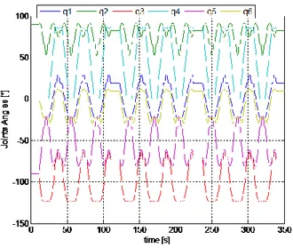
In the second experiment reported in this paper, the robot performs movements that simulate a possible realistic industrial application like grasping an object that lies in a given position , in this case at the lower right of the robot, and then it moves in another position that in this case is in the upper left. These movements involve all the joints in combination (Fig.45).
Figure 36: second experiment path
Figure 37: joint angles
As shown in the figures below, the joints that have the rotation axis parallel to the gravity suffer of a bigger error with respect to the other joints, because it is not possible to correct their estimation by means of the accelerometers measurements.
The estimation of the angle of the first joint , that as previously said is always parallel to the gravity, has a maximum error of about 2° in both EKF and PF cases.
From the results of the estimation of the angle of the first joint it is possible to see that there is a small offset between the two methods because, for its own intrinsic characteristics, the PF suffers the unfeasibility to be able to correct the estimation with the accelerometers measurements, more than the EKF.
As it is possible to see in the tables 7, 8 and 9, the estimation of the angle of the second joint has always an error approximately equal to zero with both methods.
Figure 38: angle error on the first joint
Figure 39: angle error on the second joint
Even for the angles of the third and fourth joints, that are never parallel to the gravity, the error of the estimation is very low with both methods.
0 50 100 150 200 250 300 350 -2 -1 0 1 time [s] q 1 e rr [° ] EKF PF gyros 0 50 100 150 200 250 300 350 -4 -3 -2 -1 0 1 time [s] q 2 e rr [° ] EKF PF gyros
Figure 48: angle error on the third joint
Figure 40: angle error on the fourth joint
Figure 41: angle error on the fifth joint
Figure 42: angle error on the sixth joint
The results of the estimation of the angles of the last two joints are the most interesting because, like for the second joint, it is possible to notice that the PF
0 50 100 150 200 250 300 350 -4 -2 0 2 4 time [s] q3 e rr [° ] EKF PF gyros 0 50 100 150 200 250 300 350 -4 -2 0 2 4 time [s] q 4 e rr [° ] EKF PF gyros 0 50 100 150 200 250 300 350 -4 -2 0 2 4 time [s] q 5 e rr [° ] EKF PF gyros 0 50 100 150 200 250 300 350 -6 -4 -2 0 2 4 time [s] q 6 e rr [° ] EKF PF gyros
suffer the presence of more vibrations and the parallelism with the gravity more than the EKF.
By using the PF the estimation error of the angle of the fifth and the sixth joints has a maximum value of about 4°.
As it was said before, the EKF has better performance than the PF, and in fact the estimation error of the angle of the last two joints is always below 1°.
Table 10: joints estimation error (EKF)
joint mean standard deviation root mean square max 1 0.93 0.43 1.02 1.79 2 -0.01 0.07 0.07 0.26 3 0.05 0.12 0.14 0.40 4 -0.06 0.14 0.15 0.47 5 -0.15 0.24 0.28 1.22 6 0.04 0.36 0.36 0.98
Table 11: joints estimation error (PF)
joint mean standard deviation root mean square max 1 -1.34 0.42 1.41 2.19 2 -0.01 0.08 0.08 0.29 3 0.05 0.17 0.18 0.81 4 0.02 0.23 0.23 1.03 5 -0.04 1.46 1.46 3.75 6 0.43 1.46 1.52 3.78
Table 12: joints estimation error (Gyros integration)
joint mean standard deviation
root mean square
![Table 6: joints estimation error (Gyros integration) [°]](https://thumb-eu.123doks.com/thumbv2/123dokorg/4519461.34865/63.629.144.505.146.320/table-joints-estimation-error-gyros-integration.webp)