Ecosystem respiration in a Mediterranean Turkey oak forest: eddy covariance and chamber-based models comparison

(1)

UNIVERSITÀ DEGLI STUDI DELLA TUSCIA

Dipartimento per l’Innovazione nei Sistemi Biologici, Agroalimentari e Forestali

Corso di Dottorato di Ricerca in

E

COLOGIA

F

ORESTALE XXV ciclo

“Ecosystem respiration in a Mediterranean Turkey oak forest:

eddy covariance and chamber-based models comparison”

Coordinatore Dottoranda Prof. Paolo De Angelis Claudia Consalvo

Tutor

Prof. Paolo De Angelis

(2)

(3)

Abstract

Eddy covariance and up-scaled chamber measurements were used to estimate ecosystem respiration (Reco) in a Quercus cerris L. coppice forest in Central Italy. The annual variation of Reco and its components, was analyzed in relation to seasonal changes in soil temperature and soil moisture. Chamber measurements on soil, stems and leaves were carried out between June 2010 and December 2012. Each plot was chosen to be always within the footprint of the eddy covariance tower installed in the forest compartment.

The ecosystem respiration and its main components shown a strong seasonal variability. Summer aridity played a crucial role on the observed reduction of respiration that was evident both in soil and stem CO2 efflux rates. Soil respiration (Rs) and stem respiration (Rstem)

increased from winter to spring, decreased in summer and suddenly increased in autumn after rainfall events. A different trend was showed by leaf dark respiration (Rl) that increased from

spring to summer and decreased in autumn.

Based on up-scaled chamber measurements, ecosystem respiration (Recocuv) showed a

significant temporal variation over the year. Rs and Rstem followed the same trend of

ecosystem respiration estimated by eddy covariance (Recoeddy) with a reduction during

summer months consequently to summer drought. On the contrary, Rl peaked in August and

decreased in autumn and was responsible for the decoupling of the two Reco estimates. The total annual Recoeddy chosen as reference was 9.11 t C ha-1 y-1, while the total annual

contribution of Rs, Rstem and Rl was 6.79, 1.77 and 4.74 t C ha-1 y-1, respectively. Thus, the

relative contribution of each component was 51% for the soil, 13% for the stem and 36% for leaves, confirming that whole ecosystem respiration is dominated by soil respiration. Recocuv

was 32% larger than ecosystem respiration estimated by eddy covariance.

Through model validation techniques was possible to quantify the uncertainty. The results showed that method of estimation used, sample size, and biotic and abiotic factors influencing the respiration rates, can lead to both underestimation and overestimation higher than 50%. The main contribution of errors was showed by stem CO2 efflux because of the bad model

performance during the growing period. Therefore, the sources of uncertainty identified suggest that the comparison between the estimation of Recocuv and Recoeddy, is feasible only if

the errors are minimized. An adequate sample size, use of prediction models suitable for Mediterranean environments and, standardized methods as much as possible, are needful.

(4)

(5)

Riassunto

La tecnica eddy covariance e le misure con cuvetta scalate a livello ecosistemico, sono state usate per stimare la respirazione ecosistemica (Reco) in un bosco ceduo di Quercus cerris L. in Italia centrale. La variazione annuale della Reco e delle sue componenti è stata analizzata in relazione alle variazioni stagionali di temperatura e umidità del suolo. Le misure di efflusso di CO2 con cuvetta

dal suolo, dai fusti e dalle foglie sono state effettuate tra giugno 2010 e dicembre 2012. L’area sperimentale è stata scelta per essere sempre dentro la footprint della torre eddy covariance installata nella particella forestale oggetto di studio. La respirazione dell'ecosistema e le sue componenti principali hanno mostrato una forte variabilità stagionale. L’aridità estiva ha svolto un ruolo cruciale nella riduzione di respirazione ed è stata evidente sia nei tassi di efflusso di CO2 dal

suolo che dai fusti. I tassi di respirazione del suolo (Rs) e dei fusti (Rstem) sono aumentati

dall'inverno alla primavera, sono diminuiti in estate e sono improvvisamente aumentati in autunno dopo alcuni eventi piovosi. Un andamento diverso è stato mostrato dalla respirazione fogliare (Rl),

che è aumentata dalla primavera all'estate ed è diminuita in autunno. Sulla base delle misure da cuvetta scalate, la respirazione ecosistemica (Recocuv) ha mostrato una significativa variazione

temporale nel corso dell'anno. Rs e Rstem hanno seguito lo stesso andamento della respirazione

ecosistemica stimata con la tecnica eddy covariance (Recoeddy) con una riduzione durante i mesi

estivi, a causa della siccità. Al contrario, Rl ha raggiunto un picco nel mese di agosto ed è poi

diminuita in autunno essendo così responsabile del disaccordo delle due stime di Reco. La Recoeddy

annuale, scelta come riferimento, è stata stimata pari a 9.11 t C ha-1 anno-1, mentre, il contributo totale annuo di Rs , Rstem e Rl è stato di 6.79, 1.77 e 4.74 t C ha- 1 anno-1, rispettivamente. Pertanto il

contributo relativo di ciascuna componente è stato del 51% per il suolo, del 13% per i fusti e del 36% per le foglie, confermando che la respirazione ecosistema è dominata dalla respirazione del suolo. Recocuv è stata maggiore della Recoeddy del 32%.

Attraverso tecniche di validazione è stato possibile quantificare l'incertezza delle stime. I risultati hanno dimostrato che il metodo di stima utilizzato, la dimensione del campione, e i fattori biotici e abiotici che influenzano i tassi di respirazione, possono portare sia ad una sottostima che ad una sovrastima superiore al 50%. Il contributo maggiore all’errore di stima è stato dato dall’efflusso di CO2 a causa delle cattive prestazioni del modello durante il periodo di crescita. Pertanto, le fonti di

incertezza individuate suggeriscono che il confronto tra la stima di Recocuv e Recoeddy, è fattibile

solo se sono ridotti al minimo gli errori quindi, utilizzando un campione di dimensioni adeguate, modelli di previsione adatti ad ambienti mediterranei e metodi standardizzati di misura.

(6)

(7)

3 To predict long-term trends in carbon sequestration by ecosystems, it is necessary to understand the responses of ecosystem respiration, defined as the sum of soil microbial, root, leaf and stem respiration to environmental factors (Johnson et al., 1996; Valentini et al., 2000; Vourlitis & Oechel, 1999). A consensus exists with respect to the importance of temperature and water availability in determining ecosystem CO2 emissions. Several reviews have examined the

analysis and description of temperature induced increases in soil respiration (Kätterer et al., 1998; Kirschbaum, 1995; Lloyd & Taylor, 1994). Less consistent results have been recorded with respect to the influence of soil moisture on respiration, so that different functions describing the dependence have been applied (Davidson et al., 1998; Epron et al., 1999; Fang & Moncrieff, 1999; Norman et al., 1992). Information on the processes controlling net carbon gain have often been obtained in extreme habitats, e.g. shaded, hot or cold but, respiration may be more important than photosynthesis in controlling interannual variability in net ecosystem production (Valentini et al., 2000). The Mediterranean environment is special in that prolonged drought reoccurs annually in a relatively predictable, simple manner with a long-term slow drying of the system followed by rewetting. Thus, Mediterranean sites are ideal to examine temporal changes in ecosystem carbon balance in response to soil water availability and temperature (Di Castri, 1981; Rovira & Vallejo, 1997). Long-term effects of warming and drying can only be obtained from forests in which seasonal drought is a regular feature. In order to better understand the effects of environmental factors on respiration fluxes, in the current study, stem, soil and leaf CO2 efflux of a Mediterranean deciduous species, turkey oak (Quercus cerris L.) were measured.

The study was conducted in a coppice forest in Central Italy and a comparison between the up-scaled chamber measurements and ecosystem respiration estimated by eddy covariance was carried out.

1.1 Stem CO2 efflux

Interest in stem respiration is increasing as many quantitative estimates show that it is a large component of the annual carbon balance of forest ecosystems. The stem CO2 efflux (Rstem),

accounts for 11% - 23% and 40% - 70% of the carbon assimilated in temperate and tropical forest ecosystems, respectively (Ryan et al. 1995; Chambers et al. 2004). In previous studies conducted in Mediterranean forests, Rstem varies in the range between 8% -11% (Guidolotti et al.,

(12)

4 Despite stem CO2 efflux is an important component of forest ecosystem carbon budgets and net

ecosystem CO2 exchange, little is known about Rstem in Mediterranean forests. It is important

quantify the contribution and the evolution of CO2 through the different seasons. Few studies

have examined the seasonal respiration throughout an entire year. Some have shown that the response of respiration to temperature clearly varies among months (Guidolotti et al., 2013; Paembonan, et al., 1991). Temperature sensitivity of stem respiration is usually expressed in terms of Q10 (the rate of change in respiration resulting from a 10°C increase in temperature).

Numerous studies on temperature sensitivity of stem respiration have been conducted across different forest types of the world and reported different Q10 values, varying from 1.00 to 6.40

(Acosta et al., 2011; Damesin et al., 2002; McGuire et al., 2007).

Rstem is a complex process composed of different sources of CO2 and with many controlling

factors (Teskey et al., 2008). Due to the large effect that temperature has on rates of respiration, it has often been used to predict Rstem. However, the relationships between Rstem and temperature

vary greatly. In some studies, strong correlations have been reported. For example, in different study on Pinus spp. Rstem was strongly correlated with stem temperature (Tstem) (Xu et al., 2000;

Zha et al., 2004). In other studies, Rstem was correlated with a time-lagged Tstem (Kim et al., 2007;

Lavigne & Ryan, 1997; Lavigne, 1996; Ryan et al., 1995; Acosta et al., 2008). Zach et al. (2009) found that for trees in tropical montane forest, Rstem was independent from Tstem in the wet

season, but was well correlated with Tstem in the dry season. Other studies have found weak, or

non-existent, correlations between Rstem and temperature in trees. Teskey & Mcguire (2002)

found that Rstem was poorly correlated with Tstem in Quercus alba trees, Bowman et al. (2005)

reported that diel variation in Rstem could not be explained by Tstem. Chambers et al. (2004)

reported that there was no relationship between Rstem and Tstem in Central Amazon tropical forest.

Zach et al. (2010) found that Rstem was completely uncoupled from the diel pattern of Tstem. They

observed positive, negative, and completely uncoupled relationships between Rstem and Tstem in

20 mature canopy trees during the dry season in a tropical montane forest. Taken together, these results suggest that temperature is not always a reliable predictor of Rstem.

Temperature exerts strong control on the rate of cellular metabolism but there are many other factors that can complicate the relationship between this rate and the amount of CO2 on stem

surface. Among these are the CO2 absorption and transport in the transpiration stream (Saveyn et

al., 2007a; Teskey & Mcguire, 2002), the long radial diffusion pathways of CO2 and high bark

resistance to gaseous diffusion (Ceschia et al., 2002; Stockfors, 2000), the corticular photosynthesis, especially important for young stems and branches (Cernusak & Marshall, 2000;

(13)

5 Sprugel, 1990; Wittmann et al., 2001; Wittmann & Pfanz, 2007, 2008; Wittmann et al., 2006), the cambial activity, substrate supply and growth (Damesin et al., 2002; Stockfors & Linder, 1998) and other environmental and physiological factors that either directly or indirectly affect Rstem including sap flow, phenology, stem oxygen concentration, solar radiation, and water

deficits (Aubrey & Teskey, 2009; Bowman et al., 2005; Brito et al., 2010; Damesin et al., 2002; Gruber et al., 2009; Maieret al., 2010; Meir et al., 2008; Saveynet al., 2007b; Zach et al., 2010). Within the same species, trees of different size have different stem CO2 efflux rates because size

also appears to influence Rstem. Diameter at breast height (DBH) has been found to be correlated

with Rstem in tropical and temperate forests (Bowman et al., 2005; Chambers et al., 2004; Kim et

al., 2007; Zach et al., 2008) and in a Mediterranean montane beech in Central Italy (Valentini et al., 1996). However, Kim et al. (2007) reported that Rstem in Pinus densiflora stand decreased

with increasing diameter.

Several previous studies have shown differences between stems for volume-based or area-based respiration (Sprugel, 1990; Stockfors, 2000), but these differences are rarely considered when scaling-up to the stand level. Many studies have shown differences among trees for stem maintenance and growth respiration, which were correlated to live cell volume and annual dry-matter production, respectively (Ryan, 1990). Thus is important determining the best unit of scale. The unit chosen (surface area, sapwood volume) can greatly affect the final results. Surface area, for instance, was found to be the best unit for expressing maintenance respiration of Picea abies (Stockfors & Linder, 1998) because the living cells were concentrated in the outer wood. Nevertheless, (Ryan, 1990) found maintenance respiration of Pinus contorta and Picea engelmannii was better estimated by sapwood volume. Stockfors (2000) in a study on Picea abies, showed that respiration at the breast height generally provided an acceptable estimate of respiration of the whole stem, especially if surface area was used as unit for scaling up. About the sampling height, he found that for a tree with an even distribution of living cells in the stem, scaling-up whole-year respiration by sapwood volume causes only small errors (7% - 12%) disregarding sample height. For a tree with living cells concentrated near the surface, scaling up by surface area produce an equally small error (2% - 14%) if the sample is taken at 140 cm height or higher.

Differences in stem respiration could be the result of differing site characteristics, but evaluations of stem respiration also depend on measurement and calculation methods. Quantifying the stem respiration of a forest ecosystem requires CO2 efflux measurements in the

(14)

6 local and non continuous field respiration measurements to estimates of carbon loss at the ecosystem level for the duration of one year.

Most studies concerning stem respiration have been done on conifers. Investigations of other woody species, especially deciduous broadleaved trees, need to be expanded.

1.2 Soil respiration

Soil respiration is an important component of forest carbon balance, accounting for 60% - 80% of total ecosystem respiration (Reco) and significantly affecting the interannual variability of net ecosystem production (Law et al., 1999; Law et al., 2001; Matteucci et al., 2000).

The contribution of Rs to Reco may differ among ecosystems, depending on site biomass

(Longdoz et al., 2000), vegetation type (Janssens et al., 1999) or plant age (Buchmann, 2000; Tedeschi et al., 2006).

Several biotic and abiotic factors influence soil CO2 production: soil temperature and moisture

(Epron et al., 1999; Law et al., 1999), soil organic matter quantity and quality (Coûteaux et al., 1995; Taylor et al., 1989), root and microbial biomass, root nitrogen content (Rey et al., 2002; Ryan et al., 1996), soil acidity and texture and site productivity (Raich & Schlesinger 1992; Raich & Potter 1995). Several examples of equations expressing the dependence on soil temperature (Davidson et al., 1998; Kucera & Kirkham, 1971; Witkamp, 1966) or soil water content (Carlyle & Than, 1988; Hanson et al., 1993; Rout & Gupta, 1989; Reichstein et al., 2003; Yuste et al. 2005) have already been provided. It is recognized that these factors usually account for 80% of temporal variability of soil CO2 efflux. However, no agreement, either on the

shape of the relationship (Lloyd & Taylor, 1994) or on the measurement procedure for these factors (depth, time and spatial frequency) has been achieved (Reichstein & Beer, 2008).

Temperature has been the most often studied factor influencing soil respiration and all studies confirm a nonlinear positive direct relationship between temperature and soil respiration. Several shapes have been proposed and the most commonly used are reviewed by Kätterer et al. (1998), Kirschbaum (1995) and Lloyd & Taylor (1994). The simplest is the exponential Q10 relationship

(the rate of change in respiration resulting from a 10°C increase in temperature).

Due to temperature related increases in respiration, ecosystems will become a net source of CO2

by 2050, although it is not clear which effect the drought would have on the full accounting of carbon dynamics (Cox et al., 2000). The effect of soil water status on soil respiration has been

(15)

7 described empirically via absolute or relative measures of volumetric water content and soil water potential as reviewed by Rodrigo et al. (1997). The relationship between soil water status and soil-respiratory processes is complex, since may individual processes vary with soil water content, in particular gas and solute diffusion, enzyme activities, and growth and mortality of microorganisms (Killham, 1994; Marshal et al., 1996). Also rewetting events often increase soil respiration, which can be explained by remineralization of dead biomass or by desorption processes, which make labile substrate available to microbes (Orchard & Cook, 1983). After a long soil drying and subsequent rewetting, soil respiration rates can exceed rates under well watered conditions before the drying (Birch, 1958). This effect has been found being of importance also for ecosystem carbon dynamics (Borken et al., 2003; Jarvis et al., 2007; Xu & Baldocchi, 2004). Thus, despite the obvious importance of biological control of soil respiration, empirical models have often focused mainly on the abiotic controls. Even for global and interannual variation, models are developed that predict soil respiration solely from climate variables (Raich et al., 2002; Raich & Potter, 1995).

Respect to temperature, less consistent results have been recorded about the influence of soil moisture on respiration and different functions describing the dependence have been applied: linear (Epron et al., 1999; Norman et al., 1992) exponential (Davidson et al., 1998; Fang & Moncrieff, 1999) and hyperbolic (e.g. Hanson et al., 1993).

Climatic variables determine most of the temporal variability in soil respiration at different scales (Davidson & Janssens, 2006; Janssens et al., 2001; Pregitzer et al., 2000). In this study an empirical model, originally developed to estimate ecosystem respiration, that accounts for variation in temperature and soil moisture, was fitted to the data of two years and, an evaluation of the model accuracy was performed.

1.3 Leaf respiration

A key factor in determining the biosfere’s response to global climate change is the impact of the abiotic environment on rates of leaf respiration (Ryan, 1991, Valentini et al., 2000, Atkin et al., 2008).

Leaf respiration represents a major source of CO2 release in plants. Mitochondrial respiration

produces much of the metabolic energy and carbon skeletons necessary for the growth and maintenance of plant tissues. In this process, between 25 and 75% of the carbon gained daily through photosynthesis is released into the atmosphere in the form of CO2 (Amthor, 2000).

(16)

8 In natural condition air temperatures vary diurnally and seasonally and leaf dark respiration (Rl)

is very sensitive to short-term changes in temperature (Körner & Larcher, 1988; Atkin et al., 2005; Tjoelker et al., 2001). Understanding the effect of variation in temperature on respiratory CO2 loss is fundamental for predicting plant growth in a changing global environment.However,

Rl may increases less markedly, remain unchanged or even decline in response to long-term rises

in temperature (Atkin et al., 2005).

The degree to which leaf respiration changes with temperature is highly variable, with Q10 values

varying from 1.4 to 4 (Azcòn-Bieto, 1992). Q10 values differ between species (Larigauderie &

Korner, 1995) and are influenced by the metabolic state of the tissue and the growth environment (Covey-Crump et al., 2002; Tjoelker et al., 2009). To fully predict variations in leaf respiration under field conditions, an understanding is needed on how other abiotic factors (e.g. drought) influence rates of leaf respiration at any given reference temperature and how such factors shape responses of Rl to temperature. Moderate drought often results in lower rates of Rl (Atkin &

Macherel, 2009; Flexas et al., 2005; Lawlor & Cornic, 2002), with Rl sometimes increasing in

response to more severe drought (Flexas et al., 2005; Slot et al., 2008). Drought may influence the temperature dependence of Rl depending on the duration and severity of stress, because

drought-induced restrictions of photosynthesis can reduce short-term temperature dependence of Rl (Slot et al., 2008). Rodríguez-Calcerrada et al. (2011) in a study on Quercus ilex L., a

Mediterranean tree species tolerant of drought and extreme temperatures, observed that leaf respiration decreased with increasing water deficit suggesting that drier conditions projected for the Mediterranean may attenuate the stimulation of leaf respiratory CO2 release by global

warming. Thus, how rates of Rl of deciduous trees in Mediterranean regions respond to

differences in soil moisture and air temperature is essential for reliable prediction of the impact of climate change on ecosystem functioning.

1.4 Ecosystem respiration

Two methods, widely used to estimate ecosystem respiration, are the chamber-based measurements and eddy covariance. The eddy covariance technique has provided an useful tool to continuously measure net ecosystem exchange (NEE) from hourly to daily, annual and interannual periods (Aubinet et al., 2000; Baldocchi, 2003). However, eddy covariance measurements do not provide direct information on component fluxes.

(17)

9 Chamber-based methods are most frequently used to estimate ecosystem CO2 flux due to their

low cost and ease of use (Epron et al., 1999; Lavigne et al., 1997; Ryan, 1990; Tang et al., 2008; Xu & Qi, 2001; Zha et al., 2004). Nevertheless, chamber-based measurements are only made on a small portion of the surface or biomass, and a large effort is required to collect sufficient data to scale up to the entire ecosystem. It is important that sufficiently large representative samples of components are measured in the chamber to obtain accurate estimates of average respiration rates (Janssens & Ceulemans, 1998; Janssens et al., 2001; Savage et al., 2008; Zha et al., 2007). At the same time, these samples are subjected to uncertainties associated with so-called chamber effects (Mosier & Bouwman, 1990).

To up-scale the chamber measurements predictive models are used, often based on the influence of abiotic factors on respiration rates (e.g. Guidolotti et al., 2013; Law et al., 1999; Tang et al., 2008; Wang et al., 2010a). Mathematical models have a wide-spread use in environmental applications but the applied models typically only render an approximate description of the system under study. Data from field measurements are compared with the corresponding model predictions. In its most elementary form this comparison is performed mainly qualitatively by visually inspecting the agreement between observed data and model predictions; more sophisticated approaches express the agreement between data and model quantitatively in terms of misfit measures (Janssen & Heuberger, 1995), which typically are functions of the error between measurements and model predictions. A given method may have low bias but its performance (accuracy estimation) may be poor due to the high variance. Moreover, problems of over-fitting can occur when a model is excessively complex or because the model can perform less well on a new data set than on the data set used for fitting. In order to avoid over-fitting, it is necessary to use additional techniques as cross-validation (Tetko et al., 1995).

Eddy covariance technique provide an estimation of carbon, water and energy exchanges between an ecosystem and the atmosphere without any perturbation over relatively large terrains (Foken et al., 2012). The measured net ecosystem exchange (NEE) of CO2 between the

ecosystem and the atmosphere reflects the balance between gross primary production (GPP) and ecosystem respiration (Reco). For understanding the mechanistic responses of ecosystem processes to environmental change it is important to separate these two flux components. As indicate in (Lasslop et al., 2010) two approaches are conventionally used: (1) respiration measurements made at night are extrapolated to the daytime or (2) light–response curves are fit to daytime NEE measurements and respiration is estimated from the intercept of the ordinate, which avoids the use of potentially problematic night time data.

(18)

10 Methods that rely on night-time data for partitioning may be biased due to the frequent nigh-time suppression of turbulence and dominance of advective fluxes not measured by conventional eddy covariance systems (Aubinet, 2008; Feigenwinter et al., 2004; Goulden et al., 1996). The second common approach extrapolating respiration from light-response curves conditioned on daytime data, usually does not account for the fact that NEE varies both as a function of temperature (mostly affecting Reco) and vapour pressure deficit (affecting GPP via stomatal regulation), among other factors (Lasslop et al., 2010). Lasslop et al. 2010, improved the method based on light-response curves taking into account the temperature sensitivity of respiration and the vapour pressure deficit (VPD) limitation of photosynthesis. In this way they improved the model’s ability to reproduce the asymmetric diurnal cycle during periods with high VPD, and enhances the reliability of Reco estimates given that the reduction of GPP by VPD may be otherwise incorrectly attributed to higher Reco. Lasslop et al. 2010, demonstrated that the uncertainty arising from systematic errors, such as advection, low turbolence, decoupling of the flow, differences in the footprint during the night compared with daytime or the choice of model and extrapolation, clearly dominates the overall uncertainty of the estimates. Moreover, it was shown by different authors (Aubinet et al., 2000; Goulden et al., 1996; Gu et al., 2005; Papale et al., 2006), that independently of the problems related to data acquisition, eddy flux measurements can underestimate the net ecosystem exchange during periods with low turbulence and air mixing.

Comparisons of eddy covariance and chamber-based estimations of Reco (Recoeddy and Recocuv,

respectively) have been made previously. This was often done by comparing eddy covariance Reco estimations with estimated fluxes calculated by scaling-up component fluxes measured in small samples (Goulden et al., 1996; Law et al., 1999; Tang et al., 2008). However, with respect to Mediterranean forests, the lack of comparable data on response of CO2 exchange measured

using eddy covariance and chamber-based methods presents problems for interpretation (Tang et al. 2008), especially relative to measurements taken simultaneously at the same sites using the two different methods. In this study, chamber-based measurements were used to measure the CO2 fluxes in soil, stem and foliage through the year. Furthermore, the eddy covariance system

was used as a reference for comparison with the up-scaled chamber measurements because, despite the uncertainties associated with the two methods, comparison of Recocuv and Recoeddy

may provide valuable information about ecological processes, such as patterns in carbon allocation to above and belowground forest compartments.

(19)

11

1.5 Objectives

- Examine seasonal patterns of the ecosystem respiration components in response to environmental variables.

- Extrapolate the chamber-based measurements to an annual budget of stand scale ecosystem.

- Quantify seasonal and annual components of ecosystem respiration fluxes in Quercus cerris L. coppice forest in Central Italy.

- Compare the eddy covariance technique with the chamber-based method for estimating ecosystem respiration.

- Evaluate the uncertainty of model performance to up-scale the chamber measurements. - Evaluate the uncertainty derived from the application of different u* thresholds to filter

(20)

(21)

13

(22)

(23)

15

2.1 Site description

The forest of Roccarespampani is in Central Italy, in the province of Viterbo (42°23’N, 11°55’E, 120 -160 m above sea level). The forest is a Quercus cerris L. coppice and covers over 1420 ha in a fairly flat area. The phytoclimatic zone is Lauretum. The climate is Mediterranean, with an average annual temperature of 14 °C and an annual rainfall of 750 mm. The rainfall distribution is irregular, with a drought period in summer of approximately 2 months. The cold is not intense but rather extended from November to April. The average minimum temperature of the coldest month ranges from 2.3 to 4 °C.

Q. cerris is the dominant overstorey species, but Q. pubescens L., Q. suber L. and Q. ilex L. occur sporadically. In addtion to oaks, we found Fraxinus ornus L., Ulmus minor Mill., Ostrya carpinifolia Scop., Carpinus orientalis L., Acer monspessulanum L. and A. campestre L., Pyrus communis L., Phillyrea latifolia L., Olea europea L. var. oleaster. Understorey vegetation is a Mediterranean-type macchia with shrubs of Prunus spinosa, Ruscus aculeatus, Cytisus scoparius, Colutea arborescens, Cornus mas, C. sanguinea and Crataegus monigyna, that are more dense in recently coppiced stands. The herbaceous layer is largely made up of grasses, which develop in spring, dry off in summer and regrow to some extent after the first autumn rains; in the older stands, herbs are limited to canopy gaps and is mainly composed of the following species: Hedera helix, Cyclamen hederifolium and repandum, Alliaria petiolata, Allium pendulinum, Clinopodium vulgare, Brachypodium sylvaticum, Thymus vulgaris.

Leaf flushing occurs in late April, while leaf abscission starts in December. The forest has been managed as a ‘coppice with standards’ over the last 200 years, with a rotation cycle varying between 15 and 20 years in length. Currently, the forest is arranged as a chronosequence of 45 compartments, each of about 26 ha, with coppice shoots in the range of 0–20 years. Coppicing consists of selective logging of trees in each compartment, leaving standards about every 10 m. The trees are kept for about three coppice rotations so that the oldest trees in the forest are between 45 and 60 years old. The result is a mosaic of compartments of different age-stands ranging from 0 to 20 years after coppicing.

The development and structure of the sprouts and the standards looks good, as well as the health condition of the population, which denotes the absence of standing dead trees and few signs of "decay of oak species". Nearly 100 stems (standards) per hectare are left standing at each harvest; the trees are kept for about three coppice rotations. Standards have an average diameter of 26.1 cm and average height of 17 m. Suckers have an average diameter of 11.0 cm and average height of 13 m. The diametric curve of distribution presents a bell shape asymmetrical to

(24)

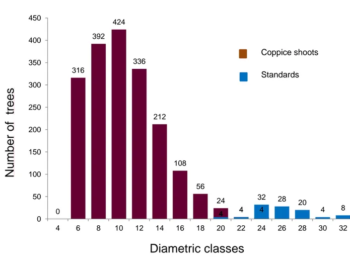
16 the right, typical of coppice with release of standards, with the highest frequencies in correspondence with the class 10. The density is equal to 3735 sprouts and 1007 stumps per hectare. The density of shoots per stump is approximately 3.7. The diametric distribution is shown in Fig. 2.1.

Fig. 2.1 - Diametric distribution of standards and coppice shoots. The distribution has the typical shape of a coppice with release of standards.

The highest root density occurs in the top 20 cm, with most roots penetrating down to 50 cm; no carbonates are present in the soil profile (Tedeschi et al., 2006).

The underlying rock is of volcanic origin and the soil is a 90 cm deep Luvisoil (FAO classification). The geological substratum is derived from the sedimentation of material of volcanic origin on pre-existing marine deposits, mostly sand. The presence of crystallized clay and the migration of clay are characteristic of this kind of soils and is a phenomenon due to the alternation of wet and dry periods.

0 316 392 424 336 212 108 56 24 4 4 4 4 32 ₂₈ 20 4 8 0 50 100 150 200 250 300 350 400 450 4 6 8 10 12 14 16 18 20 22 24 26 28 30 32

Number

of

trees

Diametric classes

Coppice shoots Standards

(25)

17 In the Tab. 2.1 are shown the results of a soil pit of 1m depth (Manca, 2003). The profile describes a well-drained soil, with an aquifer depth greater than 1 m and th1e absence of suspended aquifers on waterproof substrates. Rocky outcrops and stoniness are absent and there are no signs of erosion.

Horizon H cm 0 Litter consists mainly of turkey oak leaves

Horizon 0 cm 0-3

Abundant presence of fine roots. Lower limit with the horizon below abruptly. Lumpy texture, very friable, slightly sticky when wet; little plastic; voids and cracks absent; medium-sized pores (1-3 mm) and of Class IV (2-5%). Absent veins, crystals, concretions, nodules, carbonates cutans. Abundant biological activity, with many fine roots (25-200 of 100 cm-2). Color 5 YR 2/2 in the wet state and 5 YR 4/3 at the same dry. No skeleton.

Horizon A cm 4-23

The limit to the horizon is less clear (2-5 cm). Cracks very thin (<1 mm), fine pores (0.5-1mm) and Class III (0.5-2%); polyhedral structure sub angular, strongly developed, medium-sized (10-20 mm), compact, sticky when wet , very plastic; medium biological activity, with 10-25 fine roots to 100 cm-2, concretions of the organic type. Color 5 YR 2/4 in the wet state, 5 YR ¾ dry.

Horizon Bt cm 24-65

The lower limit is clear (2-5 cm); clayey texture; structure strongly developed, prismatic, medium; very compact; sticky when wet, plastic; limited biological activity, with 10-25 fine roots to 100 cm

-2

, often in black color and in decomposition; very thin cracks; very fine pores and of class II (0.5 - 1%); color in field 5YR 4/6, dry 5 YR 4/8.

Horizon Btx cm 66-90

The horizon is characteristic of a massive clayey frangipan. The lower limit is gradual; highly developed structure, laminated, medium, moist is very compact, wet is sticky and very plastic, the fine roots are few (1-10 100 cm-2), black and in decomposition. Organic type concretions. Skeleton appreciably from the tactile point of view; very thin cracks, very fine pores of class I (<0.1%); when wet the color is 5YR 3/6, dry is 7.5 R 5/6.

Horizon C More than 90 cm

Lower limit gradual, structured and lacking of any degree of aggregation; crumbly texture; sticky and plastic; pores and cracks absent; few roots, very fine (<1 mm); this and abundant skeleton, color 10 R ¾ and in the dry state 10 R 4/6.

(26)

18 This study is focused in a compartment of about 24 ha and the stand was 19-years-old at the beginning of the study period. In the compartment, an eddy covariance system has been running since 1998 measuring fluxes of CO2 and H2O vapour.

Fig. 2.2 - Map of the Mediterranean forest of Roccarespampani. The highlighted polygon indicates the compartment 23 in which it was carried out this study and where an eddy covariance system has been running since 1998.

2.2 Field respiration measurements: experimental layout

The main respiration components, stem CO2 efflux (Rst), soil respiration (Rs) and leaf respiration

(Rl), were measured and the measurements were carried out between June 2010 and December

2012. All the measurements were done into an area consists of a rectangular plot of about 4 ha (400 x 100 m), was chosen to be always within the flux footprint of the eddy covariance tower, according to the prevailing wind direction (Fig. 2.5). The flux footprint is an upwind area where Compartment 23

(27)

19 the atmospheric flux is generated, namely an upwind area “seen” by the instruments measuring vertical turbulent fluxes.

2.2.1

Stem CO2 efflux

In the plot of 4 ha, in the vicinity of the tower, according to the diameters distribution, 9 trees, 4 standards and 5 coppice shoots, were selected to measure stem CO2 efflux, as shown in Fig. 2.3.

The CO2 efflux were measured at the breast height (1.30 m) using a temporary clamp-on

chambers made of a transparent, hard plastic Acrylic resin. We called this efflux “stem respiration”, keeping in mind that the CO2 released in the chamber could also come from CO2

transported by the xylem, as suggested in several studies (Levy et al., 1999; Teskey & Mcguire, 2002). The chambers (Fig. 2.4) were made up of two parts: a fixed collar on the stem to 1.30 and a removable lid connected to a portable infrared gas analyzer (Li-8100; Li-cor Inc., Lincoln, NE, USA), operating in closed mode. We used nine collars 20-cm-long, 4.5 cm depth and 2 – 5 cm wide for smaller and larger diameters, respectively. During the measurements the cover was placed and fixed on collars that were permanently installed at breast height on the south-facing side of each tree stem. The edges of the chambers in contact with the bark, were covered by neoprene and sealed to the tree bark with Terostat (Henkel KgaA, Germany). A neoprene gasket was used also on the external edge of the collars and on the borders of the lids. The seals were tested by blowing along the joints and measuring the CO2 evolution in the chamber. The

chambers were connected to the IRGA (InfraRed Gas Analyzer) by flexible tubing. Before installing the chambers, the trunk was gently scrubbed in order to remove algae and lichens present on the bark. At the time of first measurement, the chamber was covered with a black cloth to evaluate CO2 refixation by the bark and no stem photosynthesis was find.

The measurements were performed at breast height because it provide an acceptable estimation of CO2 efflux of the whole stem (J Stockfors, 2000).

The stem CO2 effluxes were measured over the growing season until the beginning of the winter

2012 (April - December). We measured Rstem every 15 days, five times per day starting just after

dawn and ending at the time of maximum air temperature. The time interval between a measurement and the other was about an hour and a half. The measurement time was 90 seconds. Between measurements sets, the lids were removed from the chambers to allow air ventilation and avoid CO2 accumulation in the chambers. The stem temperature is the more biologically

(28)

20 relevant reference, so it was measured close to the chamber by an infrared thermometer (MINOLTA-LAND-CYCLOPS-COMPAC).

Fig. 2.3 – Experimental layout of stem CO2 efflux. Four standards and five coppice shoots were chosen representative the

diameter distribution in the compartment.

Fig. 2.4 – Chamber with a fixed collar on the stem to 1.30 and a removable lid connected to a portable infrared gas analyzer by flexible tubing.

(29)

21

2.2.2

Soil respiration

In 2010, within the plot of 4 ha, height rectangular subplots were randomly chosen within a regular grid of mesh 20 x 20 m. In each subplot, 5 PVC collars of 5 cm high and 20 cm in diameter (a total of 40 points) were fixed in the ground to measure soil respiration between August 2010 and August 2011 (Fig. 2.5). In 2012, a transect of 16 m in length was traced and 8 PVC collars of 5 cm height and 20 cm in diameter were fixed in the ground to measure soil respiration from January to December (Fig. 2.5). The collars had two stainless steel legs to facilitate the insertion into the ground leaving 2 cm above the soil surface.

Fig. 2.5 – Experimental layout of soil respiration. Eight subplots randomly chosen in a 4 ha area falling in the eddy covariance footprint estimated according to the prevailing wind direction.

Soil respiration was measured with a closed soil CO2 flux system (Li-8100; Li-cor Inc., Lincoln,

NE, USA) connected to 20 cm chamber. The system measures the change in CO2 concentration

inside the chamber within 90s interval.

During the Rs measurements, soil temperature at 5 cm depth (Ts) was measured with a soil temperature probe (HD 9216, DELTA OHM). Soil water content (SWC) over 5 cm depth, was measured with a soil moisture probe (Delta-T ML2). A total of 40 measurement campaigns were done; one every two weeks.

(30)

22

2.2.3

Leaf respiration

Leaf respiration was measured on four trees (Fig. 2.6), two standards and two coppice shoots, located near the tower so as to be easily accessed and collected. Four field campaigns were carried out, once a month, from June to September 2010. Three leaves per plant were collected at the same position in the canopy; as found by Hymus et al. (2005), in the same site, on the same species, the leaf respiration measured during the night was unaffected by leaf position in the canopy. The samples were collected at two different moments, pre-dawn and after sunset. The leaves were detached with petiole, placed in water and maintained at the dark while the measurement took place. The dark leaf respiration rate was measured using a portable gas exchange system (Li-6400, Li-cor Inc., Lincoln, NE, USA), fitted with a broadleaf chamber (2cm by 3cm). Respiration rates were recorded when flux readings had stabilized, typically within 3-10 min. Temperatures were manipulated at four different degrees to determine the relationship between respiration and temperature: 15, 20, 25, and 30 °C. Despite we collected three subsample leaf discs and immediately frozen theme in liquid nitrogen to estimate the total non-structural carbohydrates (TNC), some technical problems prevented leaf biochemical determinations. In 2012, during the growing season, the leaf area index (LAI) was measured, every 15 days, with a plant canopy analyzer (Li-2000, Li-cor Inc., Lincoln, NE, USA). We traced a transect of about 200 m and we marked 10 fix points, one every 20 m in which LAI was measured just before sunset under diffused light conditions.

Fig. 2.6 – Experimental layout of leaf respiration. Four plants, 2 coppice shoots and 2 standards were chosen near the tower to reach the attached leaves.

Transect for LAI measurements 100 m

(31)

23

2.2.4

Ecosystem respiration

Net ecosystem CO2 exchange, in the compartment 23 of the forest of Roccarespampani, was

measured from the meteorological tower, using the eddy covariance method (Valentini et al., 1996), since 1998. The eddy covariance system and data processing were as described by Aubinet et al. (2000). The instrumentation consisted of a sonic anemometer (Metek USA-1 standard, Germany) which measures the wind vector and air temperature, and a closed-path infrared gas analyzer sampling with 10 Hz (IRGA Li-7000, Li-cor, USA). The sonic was mounted at a height of 1.60 m above the canopy; the sample intake for the IRGA was located immediately below the sonic anemometer (distance of 20 cm). Air was sampled at a rate of 7 l min-1 into a 4 m Teflon tube of 4 mm (inner diameter). Fluxes was computed based on a 30 min averaging period.

The local meteorological conditions were recorded continuously along with the eddy covariance data.These data were measured and averaged over a 30-min period using a data logger (CR10X-TD, Campbell Inc., USA). Air temperature and relative humidity were measured using a termo-hygrometer (TTU 600, Tecno.el s.r.l., Rome, Italy) mounted at height of 16 m above the ground. Continuous soil temperatures were measured using thermistor sensors CS107 (Campbell Inc.) at depths of 0.05, 0.15 and 0.3 m. Soil moisture was measured in one vertical soil profile using the water content reflectometers (CS615-L, Campbell Inc.) installed at depth of 01 and 0.3 m. Photosynthetic Active Radiation (PAR) was measured using a net radiometer (SKP215, Skye instruments Ltd) at a height of 19.1 m and eight net radiometers (SQ110 APOGEE, USA) at a height of 1.3 m above the ground. Soil heat flux (G) was determined using two REBS Soil Heat Flux Plates (HFP01-L, Campbell Inc.) installed near the tower at depth of 0.1 and 0.3 m .

2.3 Respiration data analysis

All the data collected during the field campaign were analyzed in order to evaluate the seasonal trend of the respiration components (Rstem, Rs and Rl) and of the ecosystem respiration estimated

by eddy covariance (Recoeddy), to scale up the spot respiration measurements to annual bases,

and to quantify the uncertainty resulting from the application of predictive models, different methods of estimation.

(32)

24 All the statistical analysis and estimations of parameters by models were performed using R language (R Core Team (2012) with the support of the “car” package (Fox & Weisberg, 2010) for the validation of the models and “qualV” package (Jachner et al. , 2007) for the quantification of the accuracy.

2.3.1

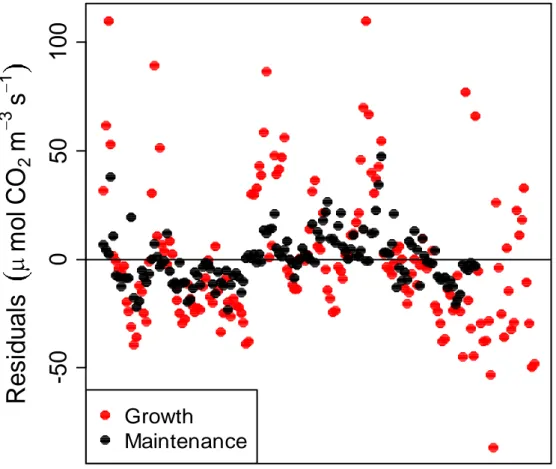
Stem CO2 efflux

The Mediterranean climate is characterized by a typical drought during the summer with a consequent decrease of the Gross Primary Production (GPP). GPP values of this period are comparable with those of the winter. Following the GPP trend, the study period of stem respiration, was divided into two different periods: the growing period from April to June and from September to the end of October and the maintenance period from July to the end of August and from November to December.

The temperature dependency of Rstem was described separately for the two different periods,

using a simple exponential equation:

Eqn. 2.1

where e are coefficients estimated by the model and Tstem is the stem temperature (°C).

To raise the scale of chamber measurements of stem respiration to the stand level for the year 2012, respiration fluxes per unit of sapwood volume were calculated based on the field measurements and with the biomass values found in the forest management plan drawn up for the forest of Roccarespampani in 2008 by (Agostini, Giuliarelli, & Petretti, 2008) and adding to the value of the biomass of 2008, the average annual growth rate (m3 ha-1 y-1) of four years. The resulting value of biomass was used to estimate stem respiration per unit ground area. Stem sapwood volume (Sa) was calculated based by the allometric equation (Eqn. 2.2) developed by Bréda, N. et al. (1993)for Quercus petraea:

(33)

25 where DBH is the diameter of the tree at the breast height.

The temperature used to scale up the spot Rstem measurements to annual bases was the air

temperature continuously measured by the thermo-hygrometer installed on the eddy tower.

2.3.2

Soil respiration

Despite the strong relationship between soil respiration and temperature, the Eqn. 2.3 (Reichstein et al., 2003) was used in order to take into account also the relationship with water availability. The modelling of soil respiration at the daily time step follows the logic that the main abiotic drivers that determine Rs are soil temperature (Ts) and soil water content (SWC) (Reichstein et

al., 2003). Eqn. 2.3 Eqn. 2.4 Eqn. 2.5 Eqn. 2.6

As explained in Reichstein et al., (2003), in these equations, (mol m-2 s-1) is the soil

(34)

26 activation-energy-type parameter of Lloyd & Taylor (1994), (°C) is the reference temperature, T0 (°C) is the lower temperature limit for the soil respiration R, and SWC1/2

(fraction) is the soil water content where half-maximal respiration (at a given temperature) occurs. In Eqn. 2.6, the temperature sensitivity of soil respiration is dependent on the soil water status of the soil, where as a first approximation E0 is linearly dependent on SWC.

Reichstein et al. (2002) corroborated the same hypothesis for ecosystem respiration. T0 was fixed at -46 °C as in the original model of Lloyd & Taylor, (1994), and was set to 18 °C, which approximates the mean soil temperature at the study sites.

2.3.3

Leaf respiration

Leaf respiration measured at 4 different temperature (15, 20, 25 and 30 °C), allowed us to estimate the temperature sensitivity of Rl. A Q10 function (Eqn. 2.7) was used to describe the

temperature dependency of Rl, and the Eqn. 2.8 to estimate the leaf respiration.

The Q10 is the temperature sensitivity of Rl (fractional change in rate with a 10 °C increase in

temperature) and k is a parameter to be estimated.

Eqn. 2.7

Eqn. 2.8

RlTb is the basal respiration rate. In our case, a basal temperature (Tb) of 20°C (RlTb = Rl20) was chosen. Air temperature were used for the variable Tair.

As reported in Tjoelker et al. 2001, models using a constant Q10 are biased, and use of a

temperature-corrected Q10 may improve the accuracy of modeled respiratory CO2 efflux, hence,

the vegetative period was divided and the model was parameterized (Eqn. 2.8) separately for each subset. Rl was estimates using the found parameters, Q10 and R20, and the air temperature

(35)

27 continuously measured by the thermo-hygrometer (TTU 600, Tecno.el s.r.l., Rome, Italy) installed on the eddy tower. The integration at canopy level was obtained by using the leaf area index (LAI) estimated by MOD15A2 that gives an 8-day-composite LAI (m2 m-2) with 1 km resolution (Oak Ridge National Laboratory Distributed Active Archive Center [ORNL DAAC]). A smoothed function based on the MOD15A2 data integrated with the data measured in the field by LI-2000 was used to interpolate the LAI on a daily scale. This smoothing function performs the computations using a locally-weighted polynomial regression. The partition of the LAI into sun and shaded leaves wasn’t performed.

Fig. 2.7 – Graphical representation of the smoothing function used to interpolate data of the LAI from MOD15A2 and LAI measured, on a daily scale.

2012-01-05 2012-04-01 2012-07-01 2012-10-01 2012-12-30 0 1 2 3 4 5 _{LAI-MODIS Smoothed} LAI-MODIS LAI Measured

(36)

28

2.3.4

Ecosystem respiration

To estimate Reco from eddy covariance data, two conventional approaches were used:

1) Respiration measurements made at night are extrapolated to the daytime; this is the method described in Reichstein et al. (2005) that introduced a new generic algorithm which derives a short-term temperature sensitivity of Reco from eddy covariance data that applies this to the extrapolation from night to daytime, and that further performs a filling of data gaps that exploits both, the covariance between fluxes and meteorological drivers and the temporal structure of the fluxes. This algorithm should give less biased estimates of gross ecosystem carbon uptake and Reco.

2) Light–response curves are fit to daytime NEE measurements and respiration is estimated from the intercept of the ordinate, which avoids the use of potentially problematic night time data. This method developed by Lasslop et al. (2010), introduced an algorithm for NEE partitioning that uses a hyperbolic light response curve fit to daytime NEE, modified to account for the temperature sensitivity of respiration and the VPD limitation of photosynthesis.

2.3.5

Statistical analysis

Repeated- measures ANOVA and Fisher’s post hoc test were used to test the seasonal variation of Rstem and to test the tree treatment (standards and coppice shoots). The Cox-Stuart test for

trend analysis and the Student’s t-test for comparison between groups of variables were used. Overall differences were considered significant with a p-value of < 0.05.

MAE (mean absolute error), MAPE (mean absolute percentage error), RMSE (root mean squared error), and r2 (coefficient of determination), were used as measures of model evaluation as defined by Janssen & Heuberger, (1995).

2.3.5.1 Model validation of Rstem and Rs

Uncertainty quantification was conducted through two different methods: k-fold cross validation and bootstrap.

In k-fold cross-validation method, the original sample is partitioned into k equal size subsamples. Of the k subsamples, a single subsample is retained as the validation data for testing the model,

(37)

29 and the remaining k − 1 subsamples are used as training data. The cross-validation process is then repeated k times (the folds), with each of the k subsamples used exactly once as the validation data. The advantage of this method over repeated random sub-sampling is that all observations are used for both training and validation, and each observation is used for validation exactly once. 10-fold cross-validation is commonly used, but in this study k was fixed equal to the number of the plants for Rstem (k = 7) and the number of the plots for Rs (k = 8). Because of

some technical problems the data of two plants were not considered.

In the bootstrap method, given a sample of size n, a bootstrap sample is created by re-sampling n cases from the data (with replacement). This method was used to evaluate the stability of the model prediction associated to different sample size. Bootstrap was then performed:

 data of stem CO2 efflux were split in subsets containing an increasing number of plants,

from 1 to 7. All the possible combinations between the plants measured, were considered and within these combinations a non-linear regression model (nls in R Core Team (2012) was run. The original data set, the one with only one possible combination (7 plants), Rstem and Tstem were randomly resampled (with replacement) 200 times and a non-linear

regression model, was run for each resample, resulting in 200 parameter estimates;

 data of soil respiration, the whole dataset of the year 2012 was split in subsets corresponding to data of 10, 15, 20, 25, 30, 35 and 40 collars. For each subset, soil respiration, soil water content and temperature were randomly resampled (with replacement) 200 times, where each resample was made up to the same number of data points as the original data subset. The non-linear regression was run for each re-sample, resulting in 200 parameter estimates.

The results of the application of the bootstrap method, were graphically analyzed, both for Rstem

and Rs, using a box-and-whisker plots.

2.3.5.2 Recoeddy: Model Efficiency selection

Concerning the Reco estimation, a source of uncertainty was evaluated due to the u* filtering. The starting dataset is NEE already corrected by storage and de-spiked (method described in Papale et al., (2006)). The u* filtering has been based on thresholds calculated using the method reported in Reichstein et al. (2005) and using 100 bootstrapped datasets.

(38)

30 - yearly (identified by the variables names with ref_y): the thresholds were found for each year and the years before; then have been put together and from this join population the final threshold was extracted (thresholds different between years).

- common (identified by the variables names with ref_c): all the thresholds found in the different years have been put together and final threshold extracted from this dataset (each year filtered with the same threshold).

In both the NEE_ref_y and NEE_ref_c, 40 NEE datasets have been created filtering the original NEE using 40 different u* values extracted from the thresholds datasets at percentiles 5, 16, 25, 50, 75, 84, 95. These 40 NEE versions have been used as basis for all the derived variables. The reference NEE was selected on the basis of the Model Efficiency. Starting from the 40 different NEE estimations it was calculated the Model Efficiency between each version and the others 39. The reference NEE was selected as the one with higher Model Efficiency sum (so the most similar to the others 39). As reference, in the 2012, were selected:

1) for the estimation of Reco by the method of Lasslop (2010) NEE_ref_c filtered using the u* percentile 36.25

NEE_ref_y filtered using the u* percentile 38.75

2) for the estimation of Reco by the method of Reichstein (2005) NEE_ref_c filtered using the u* percentile 48.75

(39)

31

(40)

(41)

33

3.1 Stem CO

2

efflux

3.1.1

Daily variation

On most days, the relationship between stem temperature and stem respiration was well described by the exponential Eqn. 2.1. The temporal variation in Rstem rates were explained by

stem surface temperature on daily scale. It reached the maximum when stem and air temperature were highest, while the minimum values in the early hours of the morning, when the temperature was lower. The relationships between stem CO2 efflux and stem temperature on daily scale, were

strong with almost always a value of R2 > 0.70. In

Fig. 3.1 are showed, the data of all plants for each date of measurement. Each curve is represented by the fit of the 5 points corresponding to the measurements of the 5 moments of the day, from just after dawn at the time of maximum daily temperature.

Fig. 3.1 – Relation between stem CO2 efflux and temperature on daily scale.

28-Apr -5 5 15 25 35 45 0 1 2 3 4 5 -5 5 15 25 35 45 0 1 2 3 4 5 -5 5 15 25 35 45 0 1 2 3 4 5 -5 5 15 25 35 45 0 1 2 3 4 5 -5 5 15 25 35 45 0 1 2 3 4 5 -5 5 15 25 35 45 0 1 2 3 4 5 -5 5 15 25 35 45 0 1 2 3 4 5 28-Jun -5 5 15 25 35 45 0 1 2 3 4 5 -5 5 15 25 35 45 0 1 2 3 4 5 -5 5 15 25 35 45 0 1 2 3 4 5 -5 5 15 25 35 45 0 1 2 3 4 5 -5 5 15 25 35 45 0 1 2 3 4 5 -5 5 15 25 35 45 0 1 2 3 4 5 -5 5 15 25 35 45 0 1 2 3 4 5 12-Jul -5 5 15 25 35 45 0 1 2 3 4 5 -5 5 15 25 35 45 0 1 2 3 4 5 -5 5 15 25 35 45 0 1 2 3 4 5 -5 5 15 25 35 45 0 1 2 3 4 5 -5 5 15 25 35 45 0 1 2 3 4 5 -5 5 15 25 35 45 0 1 2 3 4 5 -5 5 15 25 35 45 0 1 2 3 4 5 1-Aug -5 5 15 25 35 45 0 1 2 3 4 5 -5 5 15 25 35 45 0 1 2 3 4 5 -5 5 15 25 35 45 0 1 2 3 4 5 -5 5 15 25 35 45 0 1 2 3 4 5 -5 5 15 25 35 45 0 1 2 3 4 5 -5 5 15 25 35 45 0 1 2 3 4 5 -5 5 15 25 35 45 0 1 2 3 4 5 29-Aug -5 5 15 25 35 45 0 1 2 3 4 5 -5 5 15 25 35 45 0 1 2 3 4 5 -5 5 15 25 35 45 0 1 2 3 4 5 -5 5 15 25 35 45 0 1 2 3 4 5 -5 5 15 25 35 45 0 1 2 3 4 5 -5 5 15 25 35 45 0 1 2 3 4 5 -5 5 15 25 35 45 0 1 2 3 4 5 10-Sep -5 5 15 25 35 45 0 1 2 3 4 5 -5 5 15 25 35 45 0 1 2 3 4 5 -5 5 15 25 35 45 0 1 2 3 4 5 -5 5 15 25 35 45 0 1 2 3 4 5 -5 5 15 25 35 45 0 1 2 3 4 5 -5 5 15 25 35 45 0 1 2 3 4 5 -5 5 15 25 35 45 0 1 2 3 4 5 25-Sep -5 5 15 25 35 45 0 1 2 3 4 5 -5 5 15 25 35 45 0 1 2 3 4 5 -5 5 15 25 35 45 0 1 2 3 4 5 -5 5 15 25 35 45 0 1 2 3 4 5 -5 5 15 25 35 45 0 1 2 3 4 5 -5 5 15 25 35 45 0 1 2 3 4 5 -5 5 15 25 35 45 0 1 2 3 4 5 17-Oct -5 5 15 25 35 45 0 1 2 3 4 5 -5 5 15 25 35 45 0 1 2 3 4 5 -5 5 15 25 35 45 0 1 2 3 4 5 -5 5 15 25 35 45 0 1 2 3 4 5 -5 5 15 25 35 45 0 1 2 3 4 5 -5 5 15 25 35 45 0 1 2 3 4 5 -5 5 15 25 35 45 0 1 2 3 4 5 21-Nov -5 5 15 25 35 45 0 1 2 3 4 5 -5 5 15 25 35 45 0 1 2 3 4 5 -5 5 15 25 35 45 0 1 2 3 4 5 -5 5 15 25 35 45 0 1 2 3 4 5 -5 5 15 25 35 45 0 1 2 3 4 5 -5 5 15 25 35 45 0 1 2 3 4 5 -5 5 15 25 35 45 0 1 2 3 4 5 12-Dec -5 5 15 25 35 45 0 1 2 3 4 5 -5 5 15 25 35 45 0 1 2 3 4 5 -5 5 15 25 35 45 0 1 2 3 4 5 -5 5 15 25 35 45 0 1 2 3 4 5 -5 5 15 25 35 45 0 1 2 3 4 5 -5 5 15 25 35 45 0 1 2 3 4 5 -5 5 15 25 35 45 0 1 2 3 4 5 P1 P2 P5 P6 P7 P8 P9 Rst em µ mol C O2 m -2 s -1 T [°C] T [°C] T [°C] T [°C]

(42)

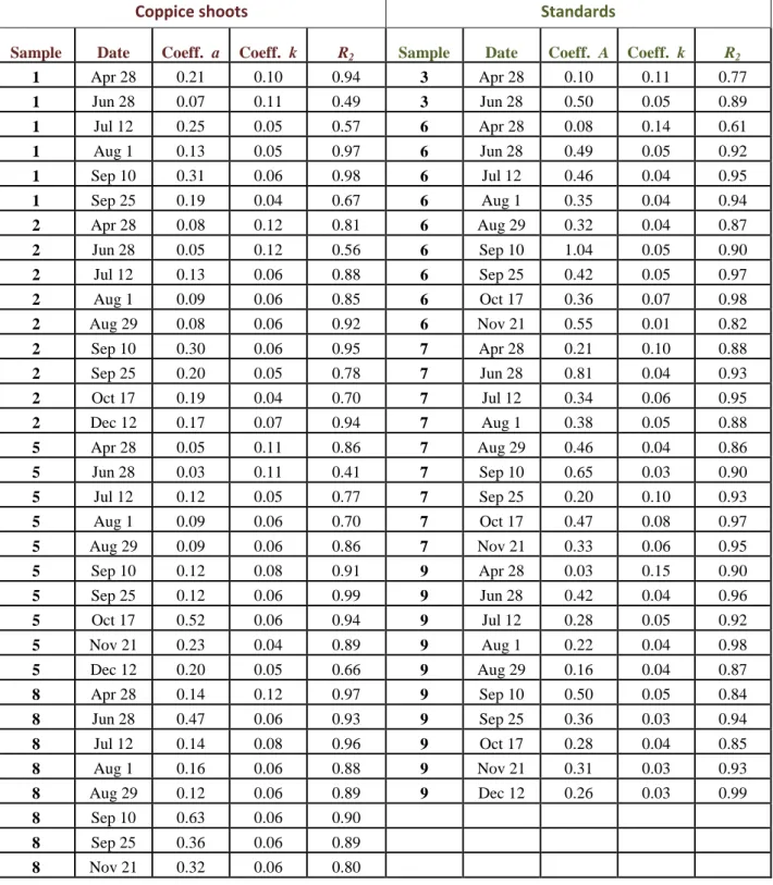
34 In Tab. 3.1 are shown the values of the parameters a and k and the coefficients of correlation (r2) of each curve. While the slope of the curve (k), on most days, for each plant, is very similar, the value of the intercept (a), during the growing period (spring and autumn), varied from 0.18 to 0.92 µmol CO2 m-2 s-1 representing the high spatial variability between individuals.

Coppice shoots Standards

Sample Date Coeff. a Coeff. k R2 Sample Date Coeff. A Coeff. k R2

1 Apr 28 0.21 0.10 0.94 3 Apr 28 0.10 0.11 0.77 1 Jun 28 0.07 0.11 0.49 3 Jun 28 0.50 0.05 0.89 1 Jul 12 0.25 0.05 0.57 6 Apr 28 0.08 0.14 0.61 1 Aug 1 0.13 0.05 0.97 6 Jun 28 0.49 0.05 0.92 1 Sep 10 0.31 0.06 0.98 6 Jul 12 0.46 0.04 0.95 1 Sep 25 0.19 0.04 0.67 6 Aug 1 0.35 0.04 0.94 2 Apr 28 0.08 0.12 0.81 6 Aug 29 0.32 0.04 0.87 2 Jun 28 0.05 0.12 0.56 6 Sep 10 1.04 0.05 0.90 2 Jul 12 0.13 0.06 0.88 6 Sep 25 0.42 0.05 0.97 2 Aug 1 0.09 0.06 0.85 6 Oct 17 0.36 0.07 0.98 2 Aug 29 0.08 0.06 0.92 6 Nov 21 0.55 0.01 0.82 2 Sep 10 0.30 0.06 0.95 7 Apr 28 0.21 0.10 0.88 2 Sep 25 0.20 0.05 0.78 7 Jun 28 0.81 0.04 0.93 2 Oct 17 0.19 0.04 0.70 7 Jul 12 0.34 0.06 0.95 2 Dec 12 0.17 0.07 0.94 7 Aug 1 0.38 0.05 0.88 5 Apr 28 0.05 0.11 0.86 7 Aug 29 0.46 0.04 0.86 5 Jun 28 0.03 0.11 0.41 7 Sep 10 0.65 0.03 0.90 5 Jul 12 0.12 0.05 0.77 7 Sep 25 0.20 0.10 0.93 5 Aug 1 0.09 0.06 0.70 7 Oct 17 0.47 0.08 0.97 5 Aug 29 0.09 0.06 0.86 7 Nov 21 0.33 0.06 0.95 5 Sep 10 0.12 0.08 0.91 9 Apr 28 0.03 0.15 0.90 5 Sep 25 0.12 0.06 0.99 9 Jun 28 0.42 0.04 0.96 5 Oct 17 0.52 0.06 0.94 9 Jul 12 0.28 0.05 0.92 5 Nov 21 0.23 0.04 0.89 9 Aug 1 0.22 0.04 0.98 5 Dec 12 0.20 0.05 0.66 9 Aug 29 0.16 0.04 0.87 8 Apr 28 0.14 0.12 0.97 9 Sep 10 0.50 0.05 0.84 8 Jun 28 0.47 0.06 0.93 9 Sep 25 0.36 0.03 0.94 8 Jul 12 0.14 0.08 0.96 9 Oct 17 0.28 0.04 0.85 8 Aug 1 0.16 0.06 0.88 9 Nov 21 0.31 0.03 0.93 8 Aug 29 0.12 0.06 0.89 9 Dec 12 0.26 0.03 0.99 8 Sep 10 0.63 0.06 0.90 8 Sep 25 0.36 0.06 0.89 8 Nov 21 0.32 0.06 0.80

(43)

35

3.1.2

Seasonal variation of stem CO2 efflux

Seasonal trend in stem respiration followed the same pattern in all trees, with the greatest rates occurring during the growing season.

The total average (±SE) of the 362 measurements of stem respiration (Rstem), carried out from

April to December 2012, was 1.23 ± 0.05 µmol CO2 m-2 s-1. On the end of the year, the lowest

CO2 efflux rates were probably caused by a cessation of growth processes and a decrease in

temperature. The highest rates of CO2 efflux were reached in spring as a result of active woody

tissue growth, high temperature and transpiration.

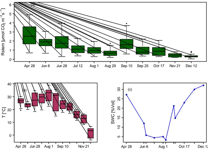
Fig. 3.2 – (a) Trend of seasonal CO2 efflux from stem surface from April to December 2012. The vertical bars indicate the

minimum and maximum values, the bottom and top of the box are the 25th and 75th percentile, the black band near the middle of the box is the median. (b) Variations of temperature during the study period. There is a marked temperature range from the early hours of the morning until shortly before midday, both in August and December. (c) Seasonal trend of soil water content over 5 cm depth.

Apr 28 Jun 6 Jun 28 Jul 12 Aug 1 Aug 29 Sep 10 Sep 25 Oct 17 Nov 21 Dec 12 0 1 2 3 4 5 6 R st e m [µ m o l C O2 m 2 s 1 ] (a)

Apr 28 Jun 28 Aug 1 Sep 10 Nov 21 0 10 20 30 40 T [° C ] (b) 5 10 15 20 25 30 S W C [ % V o l]

Apr 28 Jun 6 Aug 1 Oct 17 Dec 12 (c)