Preparing for a future satellite mission to measure wind and improve climate forecasts

(1)

ALMA MATER STUDIORUM

UNIVERSITA’ DI BOLOGNA

SCHOOL OF ENGINEERING

-Forlì Campus-

SECOND CYCLE MASTER’S DEGREE in

INGEGNERIA AEROSPAZIALE/ AEROSPACE ENGINEERING

Class LM-20

GRADUATION THESIS

In Spacecraft Orbital Dynamics and Control

Preparing for a future satellite mission to

measure wind and improve climate forecasts

CANDIDATE

Niccolò Cavicchioli

SUPERVISOR

Prof. Marco Zannoni

.

(2)

(3)

Master’s thesis

Preparing for a future satellite mission to

measure wind and improve climate forecasts

NICCOLO’ CAVICCHIOLI

In collaboration with:

DF

Department of Space, Earth and Environment

Division of Microwave and Optical Remote Sensing

Chalmers University of Technology Gothenburg, Sweden 2021

(4)

(5)

Abstract

Stratospheric Inferred Winds (SIW) is a future satellite mission, which has been se-lected by the Swedish Space Agency to become the next Swedish research satellite, to be launched in 2024. It will consist of a sub-millimetre radiometer instrument, optimised for wind measurements in the middle atmosphere, and orbiting the Earth aboard a micro satellite platform. The goal of this master thesis was to carry out a preliminary study to assess the potential of the mission to contribute to a better understanding of the middle atmospheric dynamical events, and thus to improve weather and climate forecasts. The analysis of zonal mean eastward wind from two five year-long reanalysis data sets, namely ERA5 and MERRA-2, is described and compared to SIW estimated performances. The areas of major disagreement are investigated in details. It appears that the models have important difficulties to accurately reproduce the dynamical phenomena in the regions out of geostrophic balance due to wave forcing processes. The results show that a significant contri-bution can be provided by the SIW mission particularly at low latitudes, where the effects related to the Semi-Annual Oscillation can be studied, and at high latitudes during winter-time, where the effects of Sudden Stratospheric Warming events can be investigated. In those regions, at mesospheric altitudes, SIW estimated precision is most of the time significantly lower than the observed differences.

Keywords: SIW, wind measurement, climate forecast, middle atmosphere, atmo-spheric dynamics.

(6)

(7)

List of Figures

1.1 Atmospheric layers and vertical temperature variation . . . 2

1.2 Atmospheric circulation patterns: troposphere . . . 4

1.3 Atmospheric circulation patterns: stratosphere and mesosphere . . . . 5

1.4 Zonal mean eastward wind near the equator . . . 8

1.5 Space wind measuring instruments: limb sounders . . . 10

1.6 View of the Innosat satellite . . . 13

1.7 SIW performance estimate . . . 14

2.1 Zonal Mean Zonal Wind: Spring . . . 21

2.2 Zonal Mean Zonal Wind: Autumn . . . 23

2.3 Zonal Mean Zonal Wind: Summer . . . 24

2.4 Zonal Mean Zonal Wind: Winter . . . 26

2.5 Zonal Mean Zonal Wind: Winter 2018-2019 . . . 29

2.6 Zonal Mean Zonal Wind: Winter 2019-2020 . . . 31

(10)

(11)

List of Tables

1.1 Limb sounding wind measuring instruments . . . 10 1.2 MERRA-2 and ERA5 data observations . . . 12 A.1 Space borne wind measurement instruments . . . I

(12)

(13)

List of Acronyms

AHI Advanced Himawari Imager.

AVHRR Advanced Very High Resolution Radiometer. BDC Brewer-Dobson Circulation.

C3S Copernicus Climate Change Service.

ECMWF European Centre for Medium-Range Weather Forecasts. ERA5 ECMWF ReAnalysis, version 5.

EUMETSAT European Organization for the Exploitation of Meteorological

Satel-lites.

GEOS Goddard Earth Observing System. GMS Geostationary Meteorological Satellite.

GOES Geostationary Operational Environmental Satellites. ISS International Space Station.

JMA Japanese Meteorological Agency.

LIDAR Laser Imaging Detection and Ranging. LOS Line of Sight.

MERRA-2 Modern-Era Retrospective Analysis for Research and Applications,

version 2.

MODIS Moderate-resolution Image Spectro-radiometer.

MTSAT IMAGER Japanese Advanced Meteorological Imager. MTSAT IMAGER-2 Japanese Advanced Meteorological Imager - 2. MVIRI Meteosat Visible Infra-Red Imager.

NASA National Aeronautics and Space Administration. NOAA National Oceanic and Atmospheric Administration. QBO Quasi-Biennial Oscillation.

SAO Semi-Annual Oscillation.

SEVIRI Spinning Enhanced Visible Infra-Red Imager. SIW Stratospheric Inferred Winds.

SMILES Superconducting Submillimeter-Wave Limb-Emission Sounder. SSW Sudden Stratospheric Warming.

(14)

SWIFT The Stratospheric Wind Interferometer For Transport studies. UTC Coordinated Universal Time.

VAS Visible-Infrared Spin Scan Radiometer Atmospheric Sounder. VISSR Visible-Infrared Spin Scan Radiometer.

(15)

1

Background and Motivation

Wind measurement is of fundamental importance in weather and climate forecasts. Having accurate measurements in the middle atmosphere is crucial to better predict the weather evolution and to get a deeper understanding of the major dynamical phenomena controlling the climate variability. Yet winds in this atmospheric region have up to now barely been observed. The Stratospheric Inferred Winds (SIW) mission’s goal is to satisfy this need by providing accurate data to the scientific community. This report investigates the relation between present wind data and SIW performance in different operational conditions, highlighting the areas where new data coming from SIW can set a remarkable improvement.

1.1 Atmospheric Dynamics

Planet Earth is surrounded by the atmosphere, a layer of gases trapped close to the surface due to the Earth’s gravity. Thanks to the presence of this layer of gas, part of the heat coming from the Sun is absorbed and remains near to the surface avoiding a greater variation in temperature between day and night.

1.1.1 The atmosphere and its structure

1.1.1.1 Structure

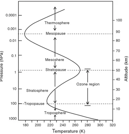
The atmosphere is made of different layers, defined according to the mean vertical thermal gradient (Kuilman, 2019, and references therein). As shown in Figure 1.1, the troposphere and the mesosphere are characterized by a negative temperature gradient, whereas the stratosphere and the thermosphere present a positive one. Those layers are separated by thin transition areas called tropopause, stratopause and mesopause, respectively. The troposphere is the closest layer to the ground, which contains about 75% of the whole atmospheric mass. The height of its upper limit decreases with latitude. It extends up to about 16 km above the equator and only 8 km above the poles. This is due to the air temperature, warmer at low latitudes and colder at higher ones, causing the air to expand or compress. Since the temperature gradient also defines the steadiness of the different layers, dynamical phenomena happening in the troposphere are generally unstable. Right on top of the troposphere, a transition region called the tropopause can be found. It is a very thin layer characterized by zero temperature gradient. The stratosphere is the first layer with stable dynamics that can be found from the Earth’s surface. It reaches about 50 km of altitude and it is the lower part of the so-called middle

(16)

Figure 1.1: Atmospheric layers and vertical temperature variation (credit:

Strato-sphere TropoStrato-sphere Interaction: An Introduction).

atmosphere. A great quantity of ozone is present here (approximately 90% of the total atmospheric ozone). The transition region between the stratosphere and the mesosphere is called the stratopause. The mesosphere is characterized by a negative temperature gradient. It reaches an altitude of about 85-100 km (varying with latitude and season), where the mesopause is located. The uppermost layer of the Earth’s atmosphere is the thermosphere. Here, at about 100 km of altitude is generally set the upper bound of the middle atmosphere. Although there is no a properly defined upper limit for the thermosphere, above it the open space can be found.

1.1.1.2 Composition

The atmosphere is mainly composed by nitrogen, N2, (∼ 78%) and oxygen, O2,

(∼ 21%). Argon (Ar), carbon dioxide (CO2), water vapour (H2O) and many other

trace gases can also be found (Vallis, 2019). The water vapor is almost entirely contained in the troposphere, while high concentration of ozone, O3, is present in

the stratosphere. The abundant presence of ozone in this part of the atmosphere is important since it absorbs the most energetic solar UV radiation, which is essential to life on Earth. It also allows accurate middle atmospheric wind measurements. Indeed, as it will be explained in Section 1.2.4, SIW wind measurements are per-formed by observing the ozone molecules carried by the moving air (Murtagh et al., 2017).

(17)

1. Background and Motivation

1.1.1.3 The middle atmosphere

The middle atmosphere is located between the lower bound of the tropopause and the lower part of the thermosphere, at about 100 km of altitude. In this region, ozone and molecular oxygen absorb ultraviolet radiation from the Sun. This rep-resents the major heating mechanism. On the other side, infrared emission from carbon dioxide, water vapour and ozone contribute to cool down the middle atmo-sphere (Kuilman, 2019, and references therein). In the middle atmoatmo-sphere, a lot of important dynamical events occur and influence the overall atmospheric behaviour. Thus, studying this part of the atmosphere is crucial to better understand weather and climate evolution on Earth.

1.1.2 Atmospheric Circulation

The atmospheric circulation describes how the heat is transferred on the planet, from warmer to colder areas. This mechanism aims at restoring thermodynamic equilibrium by means of winds. Winds are mainly driven by pressure differences and they can locally vary in time and intensity due to a number of different factors (Vallis, 2019). Coriolis acts as restoring force and partially contrasts the pressure difference: this balance is called geostrophic. Despite local variations, some big-scale patterns can be identified. The Earth’s surface presents alternating areas of high and low pressure which drive the wind close to the surface. High pressure areas can be found at about 30◦_{, 90}◦_{, whereas low pressure zones are located at 0}◦ _and

60◦ _{(Mohanakumar, 2008). Thus, they are symmetric with respect to the equator.}

The driving force is caused by the differential heating (Vallis, 2019). In fact, the curvature of Earth cause the heat flux coming from the Sun to be more concentrated near the equator and more spread out towards the poles. The area receiving more heat, called meteorological equator, moves northward during northern hemisphere summer, and southward during northern hemisphere winter. This is due to the fact that the Sun does not lay on the Earth’s equatorial plane and it causes the atmospheric circulation’s patters to depend on the seasons.

1.1.2.1 Troposphere

Near the equator, warmer and less dense air rises up to the tropopause, where it can not rise anymore because of the more stable temperature profile. It moves therefore towards higher latitudes. While moving away from the equator, the air goes through colder regions and cools down until its density increases enough to cause the air to sink towards the Earth’ surface (Mohanakumar, 2008). The air usually sinks at about 30◦ _{of latitude, both in northern and southern hemispheres.}

It gets warmer when moving downwards, due to adiabatic warming mechanism. In order to satisfy the mass conservation principle, the air travels close to the ground from 30◦ _{latitude back to the equator. Due to the Coriolis effect the air also moves}

westwards. Westward winds are also referred to as easterlies. The air warms up while moving and reaches the equator where it will restart the cycle once more (Vallis, 2019; Mohanakumar, 2008). The described patter is called Hadley cell (see Figure 1.2). Two Hadley cells are present, one in the northern and one in the

(18)

southern hemisphere. They represent the closest circulation patterns to the equator. They shift northward and southward according to the seasons. In the polar regions,

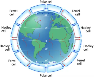
Figure 1.2: Atmospheric circulation patterns: troposphere (credit: Internet

ge-ographic). The air blows in regular patters: it rises at the equator and moves poleward, at 30° sinks and goes back to the equator (Hadley cell). Cold air sinks at the poles and travels toward 60° near the ground then it rises and moves poleward (Polar cell). In between, the Ferrel cell is characterised by air moving poleward close to the surface and opposite way in the upper troposphere. Winds close to the ground travel westward at high and low latitudes and eastward at mid latitudes. we can find the so-called Polar cells, their extension covers the polar most 30◦ _of

latitude (Vallis, 2019), i.e. 60◦ _{to 90}◦ _{in both hemispheres. Above the poles, the}

air is very cold and dense thus, it sinks towards the ground and travels close to the surface towards lower latitudes. Passing through warmer regions, the air heats up and its density decreases. This causes the air to rise at about 60◦ _{of latitude}

(Mohanakumar, 2008). From here it moves polewards and it repeats the cycle again. Ferrel cells span across mid-latitudes, 30◦ _{to 60}◦_{, in both hemispheres. There, air}

travels towards higher latitudes close to the ground and towards lower latitudes in the upper Troposphere. The near-ground wind shifts eastwards due to Coriolis effect. In the Ferrel cells the air is not driven by a major thermodynamic effect, instead, its movement is induced by the air flowing in the adjacent cells. For this reason, the polar and Hadley are called driving cells (Kuilman, 2019, and references therein). The tropospheric circulation system is symmetric with respect to the meteorological equator.

1.1.2.2 Stratosphere

The stratospheric circulation is composed of two cells, one for each hemisphere. As shown lower in Figure 1.3, the air rises at the equator and flows to the poles where it sinks. The cell in the summer hemisphere is compressed while the one in the winter

(19)

1. Background and Motivation hemisphere is stretched. The winds in the stratosphere directly affect the ozone mixing ratio, with consequences on the ozone concentration and heat absorption (Mohanakumar, 2008). The stratospheric circulation is driven by planetary waves (see Section 1.1.3.1) and it is referred to as Brewer-Dobson Circulation (BDC) (Val-lis, 2019). A region located at about 45◦_{in the winter hemisphere presents large-scale}

strong westerly winds: the polar jet stream. It is generated by strong temperature gradient in the winter hemisphere. The Polar vortex can be found between the polar jet stream and the pole. It extends from the lower stratosphere to the mesosphere and has a strong interaction with dynamic atmospheric phenomena (Kuilman, 2019, and references therein).

1.1.2.3 Mesosphere

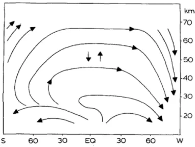
The circulation system in the mesosphere is different from the tropospheric and stratospheric ones. It is composed of a single global cell. The wind always blows from the summer hemisphere to the winter one (see Figure 1.3). The flow is stronger during summer and winter, while it is weaker during mid-seasons. There is no more symmetry with respect to the equator. Wave drag is due to gravity waves breakdown (see Section 1.1.3.1) and drives the mesospheric circulation (Kuilman, 2019, and references therein). As already mentioned in Section 1.1.2.2, the polar vortex also extends in the Mesosphere.

Figure 1.3: Atmospheric circulation patterns: stratosphere and mesosphere

(credit: American Meteorological Society). In the stratosphere, the air rises at low latitudes and sinks at higher ones (Brewer-Dobson Circulation). In the meso-sphere, the air flows from the summer hemisphere (left) to the winter hemisphere (right).

(20)

1.1.3 Dynamical processes in the middle atmosphere

Studying atmospheric dynamics in the middle atmosphere, which is controlled by a set of complex mechanisms, requires a good understanding of atmospheric waves, i.e. gravity and Rossby waves.

1.1.3.1 Atmospheric Waves

Gravity waves are oscillations produced in a stable stratified fluid and are

char-acterized by wavelength between 10 and 1000 km. Those waves can be produced by air flows over hills and mountains (orographic waves) or from instabilities, frontal systems, and thunderstorms (non-orographic waves) (Kuilman, 2019, and references therein). The restoring force is represented by buoyancy, when Coriolis force also acts as restoring force, the waves take the name of inertia-gravity waves (Kuilman, 2019, and references therein). The waves propagation depends on the zonal wind intensity, in fact, the absorption takes place only when phase speed equals the zonal wind speed. The critical level is the point where the two velocity intensity match. The forcing direction due to gravity waves depends on their breaking directions (Kuilman, 2019, and references therein). Mesospheric variability is strictly related to gravity waves. Propagation and dissipation of gravity waves in the mesosphere generates both positive and negative wave drag, leading the summer-pole to winter-pole circulation, as discussed in Section 1.1.2.3.

Rossby waves are indirectly generated by the Earth’s rotation and play an

im-portant role in large-scale meteorology (Kuilman, 2019, and references therein). Thermal forcing from sea-land interface and Earth’s topography tends to generate stationary Rossby waves of planetary scales thus, they are also referred to as plane-tary waves. Although Rossby waves can propagate both vertically and horizontally, stationary Rossby waves can propagate in the vertical direction only. In order to do that, westerlies with no excessive velocity are needed (Charney-Drazin criterion). Rossby waves only generate westward directed force due to the above mentioned criterion. Thanks to that, it is possible to understand why the Rossby waves af-fect the stratospheric eastward winter winds while summer flows are not disturbed. However, small-amplitude waves can still freely propagate during summer causing notable mixing. The mechanism throughout which the waves generate a forcing ac-tion is known as wave-breaking (Kuilman, 2019, and references therein). Since the air density decreases with height, vertically propagating waves grow in amplitude until the point where they become unstable and break. When a wave breaks, its an-gular momentum is transferred to the flow in a process called wave drag (Kuilman, 2019, and references therein). Propagation and dissipation of Rossby waves in the stratosphere generate poleward circulation (discussed in Section 1.1.2.2) (Kuilman, 2019, and references therein). Since the Rossby waves propagation mainly happens during wintertime, the stratospheric circulation is also stronger in that period.

(21)

1. Background and Motivation

1.1.3.2 Dynamical mechanisms at high latitudes

The amplitude variation of planetary waves can slow down the polar vortex and even cause the reversal from westerlies to easterlies (Pedatella et al., 2018). Such a polar vortex deformation or breakdown is associated with a major dynamical event, called Sudden Stratospheric Warming (SSW). As previously explained, when planetary waves propagate vertically, they cannot go through strong westward wind areas. For this reason, they start slowing down the air streams further below. This mechanism ends when planetary waves are no longer able to propagate vertically. A process of radiative cooling then begins and restores regular temperatures in the polar region (Pedatella et al., 2018). If the waves are able to reverse the zonal mean wind below 30 hPa a major warming occurs, otherwise it is called minor warming (Kuilman, 2019, and references therein). Major SSWs are reported to occur six times per decade in the Northern Hemisphere, while minor ones are experienced almost every winter (Pedatella et al., 2018). SSWs cause stratospheric temperatures to increase and surface temperatures to drop locally because of the cold wind blowing from the pole to lower latitudes in some regions. A better understanding of SSWs can lead to better forecast tropospheric weather.

1.1.3.3 Dynamical mechanisms at low latitudes

The Coriolis force is weaker at the equator and both gravity and Rossby waves dominate, leading to tropical anomalies and oscillation both in the Stratosphere and in the Mesosphere.

The Quasi-Biennial Oscillation (QBO) is the dominant mode of variability

at low latitudes in the stratosphere. It consists in a downward propagating easterly and westerly zonal wind regimes between about 5 hPa and the lower stratosphere. The oscillation pattern can be explained by the vertical momentum transport by equatorial gravity waves (Kuilman, 2019, and references therein). In the beginning of each cycle, strong westerly winds blow around equatorial latitudes and weaken with time, descending in altitude. Easterly winds gradually replace the westerly ones in the upper layer of the stratosphere (Stanley, 2016). Two main phases can be identified and they are characterized by the direction of the wind in the lower Stratosphere: QBO-E and QBO-W when wind blows westward and eastward re-spectively. The alternating period between QBO-E and QBO-W is of about 24 to 30 months (Kuilman, 2019, and references therein). The two phases slightly differ in intensity, downward speed and duration. QBO-E generally has more intense zonal wind and longer duration whereas, QBO-W presents faster and more regular down-ward propagation (Kuilman, 2019, and references therein). The effects of the QBO are felt also outside the tropical region, in fact, stratospheric winter polar vortex is affected by the phase of the QBO. In particular, westerly phase leads to colder and more concentrated polar vortex in the northern hemisphere.

The Semi-Annual Oscillation (SAO) is a phenomenon taking place at low

latitudes in the upper stratosphere and in the mesosphere. It consists in zonal wind and temperature oscillations and is also due to wave forcing processes in the tropical

(22)

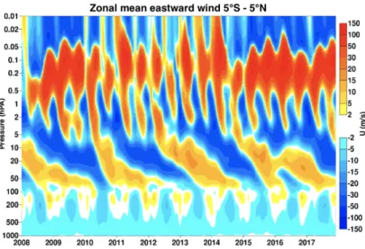
region (Murtagh et al., 2016). As it can be seen in Figure 1.4, the oscillation period is about 6 months. Maximum velocity intensity is registered in the upper stratosphere: westerly winds during equinoxes and easterly during solstices. A second peak can be identified in the upper mesosphere, having opposite phase and similar intensity with respect to the stratospheric one (Murtagh et al., 2016). The SAO and the QBO are connected, in particular, the QBO modulates both stratospheric and mesospheric SAO with effects on middle atmospheric composition and ozone distribution (Maeda, 1987).

Figure 1.4: Zonal mean eastward wind near the equator (credit: ECMWF). In the

stratosphere, below 5 hPa, we can observe the downward propagation of westerly (yellow - red) and easterly (blue) wind regimes, with a period of more or less 2 years (QBO). Further up, other oscillation features can be identified, called the stratospheric and mesospheric SAO, with a period of about 6 months.

1.2 Wind measurement

Wind is one of the representations of dynamical atmospheric processes. Knowing the intensity and direction of the wind is crucial to understand the atmospheric driving forces and to improve weather and climate forecasts. For this reason, different measuring instruments were developed in the past. Wind socks and balloons were used in the first years while lidars and radars more recently. Although providing a good accuracy, their measurements are local. The need of having a global coverage and stable measurement conditions was satisfied by the introduction of satellite-borne measuring instruments. Moreover, their operative lifetime can last more than a decade, providing a huge amount of data.

1.2.1 Satellite-borne wind measuring instruments

Satellite-borne instruments have to perform remote sensing measurements since, even the lowest orbit is hundreds of kilometers away from the wind field of interest.

(23)

1. Background and Motivation Despite different instruments have been developed through the years, the measuring principle is most of the time based on the identification of the Doppler shifts due to the movement of particles or molecules in the air (Liu et al., 2002, e.g). Every parti-cle is characterized by absorption and emission lines at specific frequencies (Schmit et al., 2005; Zieger et al., 2009). Passive sounders, like radiometers, look for emis-sion lines, while scatterometers measure the travel time of a signal, actively sent by the instrument, which is transmitted, reflected by particles and received back (Gelsthorpe R.V., 2014; Niciejewski et al., 2006; Ortland et al., 1996). Scatterome-ters measure the normalised radar back-scatter power of the previously transmitted electromagnetic pulses. This type of instruments is suitable for near-surface and ocean wind measurements (Long et al., 1993). The spatial overlapping of the sig-nals and the measurements performed at different times can provide an enhanced imaging resolution (Gelsthorpe R.V., 2014). Optical imagers combine several bands to acquire images in a process which usually takes several minutes (Schmit et al., 2005). Polarization can be changed to improve the measurements. Optical imagers are also used to detect volcanic dust clouds, clouds and moisture particles. Space Doppler wind Laser Imaging Detection and Ranging (LIDAR) detects the Doppler shifts of back scattered laser light by aerosols and other particles moving with the wind (Zhishen et al., 2003). Since the Doppler shifts are very small, high spectral resolution is needed. For atmospheric measurements up to 30 km, interferometers can be used to directly detect the shifts. Otherwise, coherent detection indirectly determines the frequency shifts at lower altitudes when using a stable laser light oscillator source (Zhishen et al., 2003). There are various possible techniques and viewing geometries to measure wind. For more details see Table A.1 of the Ap-pendix, which is listing the past, active and future space borne wind measuring instruments. SIW is a limb sounder. We are therefore going to focus particularly on this type of instruments.

1.2.2 Limb sounders

Sounder instruments are based on passive remote sensing measurement techniques, meaning that they are simply measuring signal from the atmosphere, without emit-ting radiation themselves. Limb sounders use a limb viewing geometry, i.e. have their Line of Sight (LOS) passing through the atmosphere. The great advantage of this technique is that it provides vertically resolved information on the measured quantities. This technique also ensures a relatively good signal-to-noise ratio. These instruments can perform during both day- and night-time, depending on the wave-length region in which they are measuring. Limb sounders scan the atmosphere, using moving antennas or moving platforms, allowing them to scan a greater area without loosing accuracy.

Detecting the Doppler shift of emission lines is a wind measurement technique com-monly used by limb sounders. Wind is a moving air mass which in composed by dif-ferent molecules. Usually molecular oxygen or ozone are used but this technique can also be applied to other molecules (Wu et al., 2008). The instruments can measure the emission frequency of these molecules and, by comparing it with the theoretical emission frequency, it is possible to find the Doppler shift (Murtagh et al., 2016).

(24)

This measurement gives us information about the velocity of the moving molecules along the LOS, which can be assumed to be the wind component along the LOS.

Figure 1.5: Space wind measuring instruments: limb sounders. Vertical range

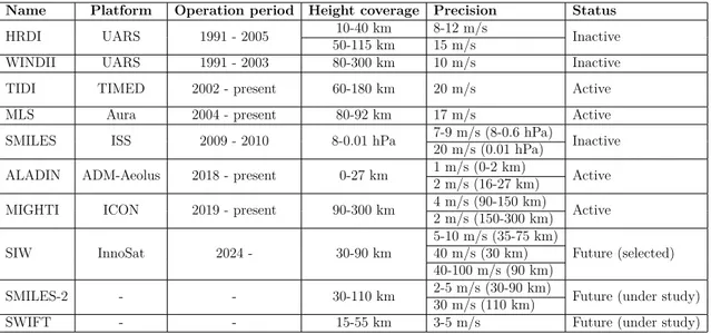
and precision of inactive (red), active (green), selected future missions (blue), and possible future missions (light blue) are represented. The altitude range is divided into two intervals: 0 to 100 km and 250 to 300 km. The width of the rectangles in the legend corresponds to a wind velocity of 6 m/s.

Name Platform Operation period Height coverage Precision Status

HRDI UARS 1991 - 2005 _{50-115 km}10-40 km 8-12 m/s_{15 m/s} Inactive WINDII UARS 1991 - 2003 80-300 km 10 m/s Inactive TIDI TIMED 2002 - present 60-180 km 20 m/s Active MLS Aura 2004 - present 80-92 km 17 m/s Active SMILES ISS 2009 - 2010 8-0.01 hPa 7-9 m/s (8-0.6 hPa)_{20 m/s (0.01 hPa)} Inactive ALADIN ADM-Aeolus 2018 - present 0-27 km 1 m/s (0-2 km)_{2 m/s (16-27 km)} Active MIGHTI ICON 2019 - present 90-300 km 4 m/s (90-150 km)_{2 m/s (150-300 km)} Active

SIW InnoSat 2024 - 30-90 km 5-10 m/s (35-75 km)40 m/s (30 km) Future (selected) 40-100 m/s (90 km)

SMILES-2 - - 30-110 km 2-5 m/s (30-90 km)_{30 m/s (110 km)} Future (under study) SWIFT - - 15-55 km 3-5 m/s Future (under study)

Table 1.1: Limb sounding wind measuring instruments. Inactive, active and future

satellite missions are included. Time period, altitude range and precision are shown. Table 1.1 and Fig. 1.5 give an overview of all the past, active and future limb sounding wind measuring instruments.

UARS and TIMED were the first two satellites carrying wind measuring limb sounders on board (WINDII, HRDI and TIDI respectively). WINDII mainly focused on the upper atmosphere with a precision of about 10 m/s (Kramer, 2002b; Gault et al., 1996; Shepherd, 1996; Banakh et al., 1995), while HRDI operated in the middle atmosphere with an accuracy of 8 to 15 m/s (Ortland et al., 1996; Swinbank and Ortland, 2003). HRDI had however a gap in the upper stratosphere (40 to 50km) where it could not measure the wind. Located on board the International Space Sta-tion (ISS), Superconducting Submillimeter-Wave Limb-Emission Sounder (SMILES)

(25)

1. Background and Motivation was designed for measuring the wind in the middle atmosphere with better accuracy than previous instruments (Baron et al., 2013). It however remained operative only for few months due to technical issues, so the resulting wind data set was relatively short.

Nowadays, four limb sounders are still operating: TIDI, MLS-Aura, ALADIN, and MIGHTI. TIDI covers an altitude range between 85 and 100 km with actual precision of 20 m/s. TIDI accuracy was expected to be better (≤ 6 m/s) but due to light leakage problem it was not able to perform at nominal conditions (Niciejewski et al., 2006). MLS-Aura was launched more than 15 years ago and it is still operative providing data between 80 and 91 km of altitude with a precision of 17 m/s (Wu et al., 2008). The only limb sounder measuring wind on ground is ALADIN, which reaches an altitude of 27 km with an extreme accuracy of 1 to 2 m/s (Kramer, 2002a). Data between 90 and 300 km are provided by MIGHTI with a precision around 2 to 4 m/s (Harding et al., 2017).

SMILES-2, Stratospheric Inferred Winds (SIW) and The Stratospheric Wind In-terferometer For Transport studies (SWIFT) are future missions: SIW has been selected and planned to be launched in the next few years, whereas, SMILES-2 and SWIFT are in a preliminary study phase and their launch is very uncertain (Ochiai et al., 2017; Baron et al., 2019; Rahnama et al., 2013). All these three missions aim to collect horizontal wind direction and intensity in the middle atmosphere, since there is a lack of global, accurate and long-term data in this altitude range (Baron et al., 2013). In particular, SIW has a good accuracy around 50 km (Baron et al., 2018), an altitude range that has up to now barely been observed. It can therefore notably improve the understanding of middle atmospheric dynamics, as we will see in Part 2 of this report.

1.2.3 Reanalysis and observations

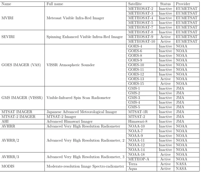
Reanalysis is used in meteorology to reprocess observations from historical unchang-ing data assimilation (Gelaro et al., 2017). This process consists in combinunchang-ing obser-vations from different sources in a consistent way. The results of reanalysis are grid-ded data-sets containing both directly and non-directly observed physical variables (Gelaro et al., 2017). Reanalysis is useful to monitor climate changes and to study atmospheric events. Satellite climate data from the 1980s have been used to pro-duce different reanalysis systems, such as ECMWF ReAnalysis, version 5 (ERA5) and Modern-Era Retrospective Analysis for Research and Applications, version 2 (MERRA-2). MERRA-2 is produced from the Goddard Earth Observing System (GEOS) atmospheric data assimilation. MERRA-2 data set covers a time period between 1980 and present days, and is continuously updated with near real-time climate analysis (Gelaro et al., 2017). ERA5 data processing is carried out by Eu-ropean Centre for Medium-Range Weather Forecasts (ECMWF). Although ERA5 reanalysis covers from 1950 to present, it is available only from 1979. This data-set is uploaded with a 5-day delay from real-time (Hennermann, 2017). As shown in Table 1.2, ERA5 and MERRA-2 have common wind data observations. However, the different assimilation and reanalysis processes give them different characteristics. Satellite missions, status and data provider are reported.

(26)

Name Full name Satellite Status Provider MVIRI Meteosat Visible Infra-Red Imager

METEOSAT-2 Inactive EUMETSAT METEOSAT-3 Inactive EUMETSAT METEOSAT-4 Inactive EUMETSAT METEOSAT-5 Inactive EUMETSAT METEOSAT-7 Inactive EUMETSAT SEVIRI Spinning Enhanced Visible Infrea-Red Imager METEOSAT-8METEOSAT-9 Inactive EUMETSATActive EUMETSAT METEOSAT-10 Active EUMETSAT GOES IMAGER (VAS) VISSR Atmospheric Sounder

GOES-4 Inactive NOAA GOES-6 Inactive NOAA GOES-8 Inactive NOAA GOES-9 Inactive NOAA GOES-10 Inactive NOAA GOES-11 Inactive NOAA GOES-12 Inactive NOAA GOES-13 Active NOAA GOES-15 Active NOAA GMS IMAGER (VISSR) Visible-Infrared Spin Scan Radiometer

GMS-1 Inactive JMA GMS-2 Inactive JMA GMS-3 Inactive JMA GMS-4 Inactive JMA GMS-5 Inactive JMA MTSAT IMAGER Japanese Advanced Meteorological Imager MTSAT-1R Inactive JMA MTSAT-2 IMAGER MTSAT-2 Imager MTSAT-2 Inactive JMA AHI Advanced Himawari Imager Himawari-8 Inactive JMA AVHRR Advanced Very High Resolution Radiometer NOAA-10 Inactive NOAA AVHRR/2 Advanced Very High Resolution Radiometer, 2

NOAA-7 Inactive NOAA NOAA-9 Inactive NOAA NOAA-11 Inactive NOAA NOAA-12 Inactive NOAA NOAA-14 Inactive NOAA AVHRR/3 Advanced Very High Resolution Radiometer, 3 NOAA-18_METEOP-A Active_Active NOAA_NOAA MODIS Moderate-resolution Image Spectro-radiometer Terra_Aqua Active_Active NASA_NASA

Table 1.2: MERRA-2 and ERA5 data observations. Wind measuring instruments

providing the observation data for ERA5 and MERRA-2 with satellite mission name, status and provider (WMO, 2011)

Observations come mainly from three data provider: European Organization for the Exploitation of Meteorological Satellites (EUMETSAT), National Oceanic and Atmospheric Administration (NOAA), and Japanese Meteorological Agency (JMA) (WMO, 2011). Meteosat Visible Infra-Red Imager (MVIRI) and Spinning Enhanced Visible Infra-Red Imager (SEVIRI) have been used on several generations of ME-TEOSAT. SEVIRI is still active, while MVIRI is not. Geostationary Meteorological Satellite (GMS) IMAGER Visible-Infrared Spin Scan Radiometer (VISSR) were used by the Japanese Meteorological Agency (JMA) before Japanese Advanced Me-teorological Imager (MTSAT IMAGER), Japanese Advanced MeMe-teorological Im-ager - 2 (MTSAT IMAGER-2), and Advanced Himawari ImIm-ager (AHI). Goddard Earth Observing System (GEOS) IMAGER Visible-Infrared Spin Scan Radiometer Atmospheric Sounder (VAS) has been used by US National Oceanic and Atmo-spheric Administration (NOAA) on several satellites of the GOES family. NOAA also used several versions of Advanced Very High Resolution Radiometer (AVHRR). Moderate-resolution Image Spectro-radiometer (MODIS) are on-board the most re-cent satellites from National Aeronautics and Space Administration (NASA). In the table it can be seen that a lot of these instruments are no longer active, since both

(27)

1. Background and Motivation reanalysis programs have been active for many years.

1.2.4 Stratospheric Inferred Winds

Stratospheric Inferred Winds (SIW) is a future space mission from the Swedish National Space Agency (Rymdstyrelsen). A limb sounder instrument is planned to be launched in 2024 on board a small satellite platform called Innosat.

1.2.4.1 Scientific motivation

SIW mission is designed to measure wind fields, temperature, and constituents con-centration in the middle atmosphere on a daily basis. The acquisition of these data will allow deeper investigations of atmospheric wave structures and dynamical events such as QBO, SAO and SSW (Murtagh et al., 2017). This mission is crucial because it focuses on a vertical range where nowadays there are only few observational data. SIW will be able to provide wind measurements between 35 and 70 km, with high accuracy in particular in the upper stratosphere and lower mesosphere, between 50 and 60 km of altitude.

1.2.4.2 Wind measurements

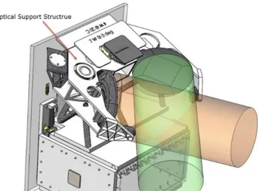
Figure 1.6: View of the Innosat satellite (credit: Omnisys instruments co.). In

the upper part (the scientific payload), two identical Gregorian telescopes mounted perpendicularly receive the electromagnetic waves emitted for the different molecules in the middle atmosphere. The two corresponding fields of view are shown in red and green. In the lower part is located the service module platform.

SIW wind measuring instrument is a microwave limb sounder which is based on the Doppler shift measuring principle (Murtagh et al., 2016). The frequency shift of the ozone thermal emission lines provides information on the molecule velocity along the line of sight. Since the observed ozone molecules are moving into the wind,

(28)

their velocity are assumed to be equal to the wind speed. SIW will operate in the sub-millimetre region and will observe a cluster of ozone lines at frequencies around 665 GHz. This will allow accurate measurements with minimum error at 55 km of altitude (Murtagh et al., 2016). As shown in Figure 1.6, two identical Gregorian telescopes with 30 cm diameter will be manufactured in aluminum. They have to be perpendicularly installed in order to measure both horizontal wind components. The reflector antennas will have a 5 km vertical field of view, and they will perform a continuing limb scan with a velocity of 0.05◦_{/s (Murtagh et al., 2016, 2017). This}

instrument will be built by Omnisys instruments co.

SIW performance depends on latitude, season and local time (see Figure 1.7).

If the zonal variation of the mean atmospheric state is assumed to be negligible, the only parameters affecting the measurements are temperature, pressure, O3, H2O,

and HCl profiles (Baron et al., 2018). Both day- and night-time estimated precision follow the same trend: reach a minimum at around 0.3 hPa, and increase at higher and lower pressure levels. The best performance achieved by SIW is about 5-7 m/s, and is lower than 10 m/s within a large pressure range: 0.02 to 2 hPa during night-time and 0.09 to 2 hPa during daynight-time. Below 2 hPa both curves quickly reach high error values for all latitudes (around 90 m/s at 10 hPa), while above 0.01 hPa the precision related to night-time measurements presents a slower increase than the daytime precision, and varies a lot as a function of latitude.

Figure 1.7: SIW performance estimate. Representation of daytime (right) and

nighttime (left) estimated performances as a function of latitude and pressure level.

SIW calibration is performed using two reference loads: the cosmic background

as cold load and a 300K-load as hot one (Murtagh et al., 2017). Both telescopes use the same reference loads, the calibration procedure is simple and reliable and it is performed at each turnaround.

1.2.4.3 Mission parameters

The limb sounding instrument will be installed on Innosat, a small satellite platform, developed by OHB Sweden and ÅAC Microtec. The satellite will orbit at about 550

(29)

1. Background and Motivation km above the Earth surface, in a retrograde sun-synchronous orbit with an inclina-tion of 98◦ _{(Baron et al., 2018). The latitude range covered by the measurements}

will be 65◦_{N - 82}◦_{S, determined by the local time of ascending node (6:00) (Baron}

(30)

(31)

2

Data analysis

Data based on easterly (and westerly) wind velocities can be processed in a number of ways to investigate different atmospheric features and dynamical events. The description of the datasets used in this study, of the analysis processes and of the results are provided in this chapter.

2.1 Data-set characteristics and data preparation

MERRA-2 and ERA5 are the two main datasets used in this study. As described in Section 1.2.3, they represent the result of the reanalysis from satellite observations. Since they have different structures, data rearrangement is necessary before being able to compare them in a meaningful way. The third dataset consist of results from a simulation study whose goal was to assess SIW measurement performance. It has a completely different structure compared to MERRA-2 and ERA5. For this reason it also requires to be interpolated in a common reference grid.

2.1.1 ERA5

ERA5 has been developed by Copernicus Climate Change Service (C3S) and pro-duced using 4D-Var data assimilation (Hennermann, 2017). ERA5 vertical grid presents 137 non-equispaced pressure levels, spanning from ground (1013.25 hPa) to 0.01 hPa. Latitude and longitude grids respectively range form 90°N to 90°S with 0.5° steps, and from 0° to 359.375°E with 0.625° steps. In this study, we are using instantaneous simulations at two specific times: 09:00 and 21:00 Coordinated Universal Time (UTC). U (eastward) and V (northward) wind values are there-fore provided at each point of the 576x361x137x2 daily grid. Expressed in m/s, wind velocity variables are of type int16 and have to be re-scaled after applying an offset. Every ERA5 file cover a month thus, they have different time-grid dimen-sions, velocity offset values and re-scaling factors. A problem related to the data production causes velocities to have unreasonable low values at the poles (90°N/S) (Hennermann, 2017). ERA5 data are provided in netCDF format.

2.1.2 MERRA-2

MERRA-2 is based on the Goddard Earth Observing System (GEOS) atmospheric data assimilation system (Gelaro et al., 2017). MERRA-2 files, like the ERA5 ones, are produced using 4D-Var data. Grid dimension of the 4D-Var is 576x361x72x8 for

(32)

each day. Time resolution is of 3 hours, starting from 00:00 UTC. MERRA-2 vertical grid presents 72 non-equispaced pressure levels, spanning from 958 to 0.015 hPa. In addition to the pressure levels, MERRA-2 provides also the corresponding altitude values in meters. Latitude and longitude grids respectively range form 90°S to 90°N with 0.5° steps, and from 180°W to 179.357°E with 0.625° steps. U/V wind values are provided at each point of the 576x361x72x8 daily grid. MERRA-2 wind velocities do not need to be re-scaled. The MERRA-2 data set consists in a netCDF file for each day. The dataset used in this study is referred to as inst3_3d_asm_Nv. As the name suggests, the data are based on instantaneous measurements. tavg3_3d_asm_Nv contains the corresponding three-hour time-averaged data collections (Bosilovich and Suarez, 2016). Daily mean values from time-averaged data have also been used as a reference to better underline the features of particular events. MERRA-2 data cover a time period from January 1980 to February 2020.

2.1.3 Comparison

The two datases involved in the analysis present some similarities such as format, and longitude/latitude grid dimensions and steps. However, upper and lower pres-sure levels, time grid, longitude and latitude limits are not the same. Moreover, MERRA-2 vertical grid is calculated and provided for each file thus, it is affected by atmospheric state and evolution during the assimilation time interval. Instead, ERA5 uses the same vertical grid which can be easily calculated using two vectors of coefficients. For these reasons, data need to be rearranged on a common grid in order to be analysed with the same procedure (see Section 2.1.5.2).

2.1.4 SIW performance estimation

SIW single-scan precision data are provided by the scientific team who carried out the study on limb sounder estimated performances. The vertical grid spans from about 240 to 0.0006 hPa with a non homogeneous 70-point distribution. Data are given for a number of latitudes, namely 80°N/S, 70°N/S, 60°N/S, 40°N/S, 20°N/S and 0° (Baron et al., 2018). Wind speed precision for both night- and daytime are provided for each point of the pressure-latitude grid (see Section 1.2.4, Figure 1.7). SIW estimated precision values are representative of horizontal wind speed intensity and not of wind direction.

2.1.5 Data preparation

2.1.5.1 Reference space and time grid

The need to define a common spatial and temporal grid, to be used for the data-sets involved, had to be fulfilled before processing the data. Averaged January 2019 MERRA-2 was chosen as a spatial grid reference: longitudinal and latitudinal bins were unchanged while some vertical values had been modified. The reason for this decision was due to the fact that the MERRA-2 vertical grid is a subset of the ERA5 one. In this way, MERRA-2 data remained almost unchanged and ERA5 ones were basically cropped. Applying an offset to the longitudinal grid and flipping

(33)

2. Data analysis the latitudinal grid were then the two only steps needed to match the ERA5 grid with the MERRA-2 one. As mentioned in Section 2.1.1, a problem caused the poles latitude (90°N/S) to be excluded from the analysis. The temporal reference is the grid from ERA5, since it is the one with less daily data available. Some pressure values of notable interest for the analysis replaced their closest one in order to have wind velocities expressed at specific levels. The whole data analysis has been carried out based on the following reference grid:

• latitude: 89.5°S to 89.5°N with 0.5° steps;

• longitude: 180°W to 179.357°E with 0.625° steps;

• vertical: 958 to 0.02 hPa, with near exponential spacing; • time: 9:00 and 21:00 UTC.

2.1.5.2 Rearranging data

Data from MERRA-2 and ERA5, as well as SIW estimated precision, have been interpolated on the vertical reference grid. Spline is the method applied in all the interpolating processes involved in the analysis. It exploits the piecewise cubic spline interpolation algorithm. This method was chosen among the different options provided by the Matlab built in function interp1 as it was a good trade off between variable shape preservation and computational cost. Since SIW operative vertical range is smaller than the reference grid, the estimated precision data have been interpolated from about 226 hPa to the upper limit (0.02 hPa). An offset of 180° W has been applied to ERA5 longitude, while latitude grid has been flipped, before removing the outermost values. U/V values from ERA5 have been re-scaled and converted to variables of type single. Since SIW northern most latitude points are around 65°N, the estimated precision data corresponding to higher latitudes were not used in the analysis.

2.2 Data analysis

In this study, the ERA5 and MERRA-2 wind reanalysis data were compared with each other, in different ways, as described below. We focused on the zonal wind, rather than on the meridional wind, because U values are significantly bigger than V values, and are more representative of dynamical features in the atmosphere. The observed differences were interpreted in light of SIW estimated precision, in order to evaluate the ability of the future SIW wind measurements to improve the representation of atmospheric dynamics by the models.

2.2.1 Global Seasonal Comparisons

Analysing the global differences for the four seasons was done as a first step, in order to investigate the areas and seasons where the models present the biggest differences. Global features strictly depend on seasons thus, it is good to look at different di-rections during different months. The analysis is based on zonal daily averages for a five-year period, from January 2015 to December 2019 on a latitude-altitude grid. The seasons are named according to the northern hemisphere convention: spring

(34)

(March to May), summer (June to August), autumn (September to November), and winter (December to February). Westerly winds from both ERA5 and MERRA-2 are day-by-day averaged. They are then presented in two independent panels as function of latitude (positive values corresponding to northern hemisphere) and al-titude (expressed in hPa and km). A third panel represents the difference between ERA5 and MERRA-2 (ERA5 - MERRA-2), hereinbelow noted ∆U. Here, SIW estimated precision is also shown. The estimated precision from SIW is obtained by interpolation both on pressure levels and on latitudes (226 to 0.02 hPa and 80°S to 65°N). Night-time and daytime values are represented. To help the visualization of main wind patterns, isolines corresponding to ±20 m/s are shown. Moreover, the areas where |∆U| is larger than SIW precision are highlighted (non-hatched).

(35)

2. Data analysis

2.2.1.1 Spring

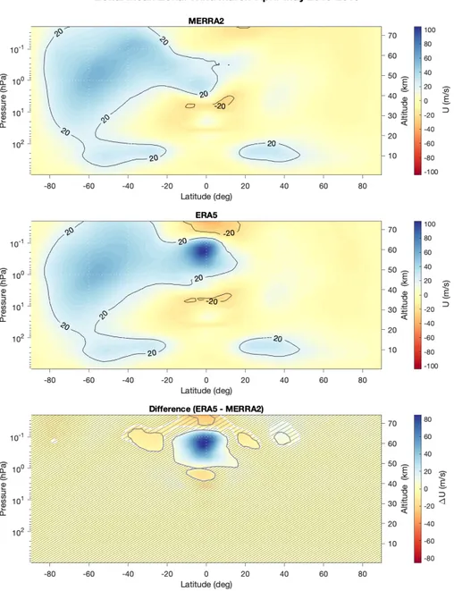
Figure 2.1: Zonal Mean Zonal Wind: Northern spring. MERRA-2 and ERA5

zonal mean zonal wind averaged for March, April and May, from 2015 to 2019, are represented in the two upper panels. Positive values of U represent eastward winds while negative velocities indicate westward ones. Contour lines corresponding to ±20 m/s show the main wind features. In the lower panel, the difference (ERA5 -MERRA-2) is shown. Non-hatched areas indicate where SIW estimated precision is lower than |∆U|. Grey and white contour lines correspond to SIW day- and night-time precision, respectively.

Spring (March, April and May) zonal mean zonal winds are represented in Figure 2.1: MERRA-2 (top), ERA5 (middle) and their difference (bottom). In the upper

(36)

panel, an area of eastward wind (blue) with velocities higher than 20 m/s is located in the northern hemisphere between 20°N and 40°N and 10 to 20 km. A symmetric eastward winds area is present in the southern hemisphere. These features are associated to the two cells of the Brewer-Dobson circulation in the stratosphere, as described in 1.1.2. The air moving poleward is deviated in the eastward direction due to the Coriolis force. In the southern hemisphere, this eastward wind area also extend to mesospheric altitudes spanning almost all negative latitudes. Westward winds around 35 km can be found between 10°S and 10°N. Similar features can be seen in the ERA5 representation (middle panel) with stronger peak velocities at about 60 km above the equator. Another relatively strong westward winds area appears in the ERA5 data set above the equator near 0.02 hPa. As it can be seen in the lower panel, high values of |∆U| are at low latitudes (20°N-20°S) above 40 km and also between 40°S and 50°N above 60 km. SIW estimated precision is represented by patches, in particular, non-hatched areas indicate where it is lower than |∆U|. Grey and white contour lines show the boundary for daytime and night-time precision, respectively.

2.2.1.2 Autumn

Autumn (September, October and November) zonal mean zonal winds are repre-sented in Figure 2.2: MERRA-2 (top), ERA5 (middle) and their difference (bot-tom). As shown in the upper panel, eastward winds (blue) can be found again in both hemispheres between 20° and 40° in the altitude range spanning from 10 to 20 km, with southern ones extending more south and to higher altitude. Westerlies are also located above 40 km spanning almost all latitude of the northern hemisphere. Similar patterns can be found in the middle panel (ERA5) with higher peaks at about 55 km above the equator. 10 to 15 km above the strongest westerlies, west-ward winds are present. In the lower panel, the non-hatched areas indicate where |∆U| is greater than the SIW estimated precision. They are at low latitudes (20°S-20°N) above 40 km, while above 60 km an area corresponding to 30° is present in both hemispheres. Grey and white contour lines show the boundary for daytime and night-time precision, respectively.

Comparing spring and autumn (Figure 2.1 and 2.2), it can be seen that |∆U| in both seasons present similar characteristics, with one more area of important differences at higher latitude in March-May, though.

(37)

2. Data analysis

Figure 2.2: Zonal Mean Zonal Wind: Northern autumn. MERRA-2 and ERA5

zonal mean zonal wind averaged for September, October and November, from 2015 to 2019, are represented in the two upper panels. Positive values of U represent eastward winds while negative velocities indicate westward ones. Contour lines corresponding to ±20 m/s show the main wind features. In the lower panel, the difference (ERA5 - MERRA-2) is shown. Non-hatched areas indicate where SIW estimated precision is lower than |∆U|. Grey and white contour lines correspond to SIW day- and night-time precision, respectively.

(38)

2.2.1.3 Summer

Summer (June, July and August) zonal mean zonal winds are represented in Figure 2.3: MERRA-2 (top), ERA5 (middle) and their difference (bottom).

Figure 2.3: Zonal Mean Zonal Wind: Northern summer. MERRA-2 and ERA5

zonal mean zonal wind averaged for June, July and August, from 2015 to 2019, are represented in the two upper panels. Positive values of U represent eastward winds while negative velocities indicate westward ones. Contour lines corresponding to ±20 m/s show the main wind features. In the lower panel, the difference (ERA5 -MERRA-2) is shown. Non-hatched areas indicate where SIW estimated precision is lower than |∆U|. Grey and white contour lines correspond to SIW day- and night-time precision, respectively.

(39)

2. Data analysis The two eastward wind areas at mid-latitudes in the stratosphere, associated with the Brewer-Dobson circulation, can be seen again, with significantly stronger wind speeds in the winter hemisphere. In the mesosphere, westward wind is present above 30 km in the summer hemisphere, it extends and gets stronger with altitude and latitude. The prevailing wind direction in the winter hemisphere is eastward, covering almost all latitude and altitude considered, with peak velocities around 40°S and 1 hPa. These patterns are explained by the thermal wind, corresponding to the change in geostrophic wind with altitude due to latitudinal temperature differences (see 1.1.2). Low latitudes are characterized by an alternating between westerly and easterly winds of moderate intensity. Similar wind structure can be found in the ERA5 panel, but stronger winds at low latitudes above 55 km can be observed, though. The lower panel shows the difference between ERA5 and MERRA-2. Here, above 45-50 km, areas of high |∆U| can be identified: mid latitude in southern hemisphere, low latitudes and mid to high latitudes in the northern hemisphere. SIW estimated precision is lower than |∆U| in these regions.

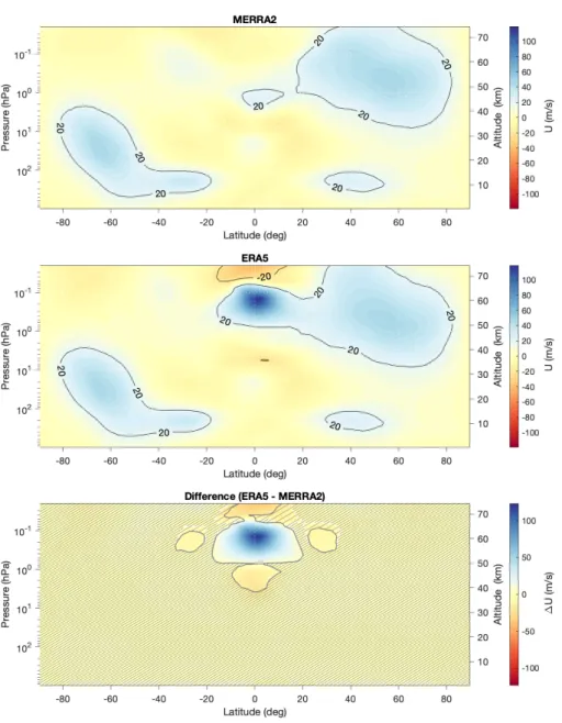
2.2.1.4 Winter

Winter (December, January and February) zonal mean zonal winds are represented in Figure 2.4: MERRA-2 (top), ERA5 (middle) and their difference (bottom). East-ward winds can be found below 25 km in both hemisphere for both ERA5 and MERRA-2: 20°N to 45°N and 25°S to 60°S. As for the other seasons, these features are associated with the stratospheric large-scale circulation. The main features of MERRA-2 and ERA5 are highlighted by iso-lines corresponding to ±20 m/s. Above 20-25 km and northern than 60°N westerly winds are present, its southern bound moves southern with altitude. In the summer hemisphere, a zone of westward winds spans almost all negative latitudes above 10 hPa. Like in the period June-August, these patterns are explained by the thermal wind balance, with typically strong westerlies in the winter hemisphere and strong easterlies in the summer hemisphere. Alternating westward and eastward zonal mean zonal wind directions characterize the latitudes around the equator. MERRA-2 presents weak wind velocities in this region while ERA5 shows stronger intensities, in particular, around 60 km where a strong peak is registered. In the lower panel, |∆U| is larger than SIW estimated precision at low altitudes above 50 km and from 40°S to 70°S above 0.2 hPa. Com-paring summer and winter plots (Figure 2.3 and 2.4), in the winter hemisphere westerly winds reach lower altitude than summer hemisphere easterlies (MERRA-2). Eastward winds are connected to low altitude winter structures in both seasons, even if during Northern winter they have weaker intensity, because the zonal mean circulation is disturbed by a more intense wave activity. Summer easterlies extends above 25-30 km, they have stronger intensity in the southern hemisphere summer as the low altitude structure in the same hemisphere. Alternated westward/eastward direction above the equator: westward below 25 km, between 30 and 55 and above 65 km, eastward otherwise. During June to August these areas are shifted down of about 5 km for both data-sets. Similar features can be found looking at ERA5, despite of weaker eastward winds in the northern hemisphere winter and in stronger peaks above the equator. In the difference panels, above 1 hPa at low latitudes high values of |∆U| can be seen during both seasons, with differences greater than SIW

(40)

estimated precision. These areas are symmetric with respect to the equator, as well as zones at higher latitudes in July-August. In December-February, a strong |∆U| is present in the southern hemisphere and it is not in the northern one.

Figure 2.4: Zonal Mean Zonal Wind: Northern winter. MERRA-2 and ERA5

zonal mean zonal wind averaged for December, January and February, from 2015 to 2019, are represented in the two upper panels. Positive values of U represent eastward winds while negative velocities indicate westward ones. Contour lines corresponding to ±20 m/s show the main wind features. In the lower panel, the difference (ERA5 - MERRA-2) is shown. Non-hatched areas indicate where SIW estimated precision is lower than |∆U|. Grey and white contour lines correspond to SIW day- and night-time precision, respectively.

(41)

2. Data analysis

2.2.1.5 Results

The global season comparison clearly shows the strong dependence of the atmo-spheric circulation on time (see Section 1.1.2.3). In fact, overall winds are stronger during the solstice seasons, even if intense confined peaks can also be observed dur-ing mid seasons. Easterly winds are particularly strong in summer and winter while, in autumn and spring, they are very weak, slower 20 m/s almost all the time. East-ward winds stronger than 20 m/s cover large areas in all seasons. Polar jet streams are present all year long in both hemispheres, its westerly winds keep a strong inten-sity during 3 seasons while it decreases in inteninten-sity and extension during summer in the northern hemisphere (see Section 1.1.2.2). SIW estimated performance is lower than the |∆U|, ERA5 minus MERRA-2, at low latitudes in the upper mesosphere all year long, and also at higher latitudes around the solstices. SIW will have a good enough precision to help improving the wind simulations and thus reducing the discrepancies between the models, in the upper mesosphere in the tropical region all year long. QBO and SAO characterise the variability of this region (see Section 1.1.3.3) and they are further investigated in Section 2.2.3. In winter and summer, areas of high |∆U| values are also observed at higher latitudes. There, SIW can contribute to improving the wind data accuracy and help to better understand the so-called SSW (see Section 1.1.3.2). For this reason, it was decided to investigate in more details high latitudes, 60°N - 65°N, during winter months in the northern hemisphere (see Section 2.2.2).

2.2.2 Winter high latitudes comparison

Winter is a very active season in terms of dynamical events. For this reason, it is meaningful to look closer to what happens at high latitudes. As mentioned in Section 2.2.1.5, during winter at polar latitudes, there are areas where SIW can help improving wind measurements and better understanding events such as SSW. The analysis therefore focuses around SIW northern most operative latitudes, 60° to 65°N, during winter months. In order to investigate how useful can the future SIW wind measurements be in this particular region and season, a major SSW event, that occurred during the Northern winter 2018-2019, was compared with the follow-ing winter, characterised by a particularly stable polar vortex. These two winters correspond to opposite situations, on a dynamical point of view. They have been analysed in the same way and the results are provided in separate sections and com-pared in the end. Winter data are processed from December 1st _{to the end of the}

following February. ERA5 and MERRA-2 are presented in separate panels. Isolines corresponding to 0 m/s are shown in order to highlight the wind direction. Differ-ences between the two reanalysis data sets are also shown in a third panel, where a grey contour line indicates the SIW nighttime estimated precision in the middle of the considered latitude band (62.5°N). Non-hatched zones correspond to |∆U| ≥ SIW precision. 2D plots are used to look in more details at particular pressure lev-els: 0.02, 0.1 and 0.6 hPa. For each level, ERA5 and MERRA-2 zonal mean zonal wind velocities for the winter under consideration are shown along side with winter zonal wind climatology and the corresponding standard deviation. Despite having separate plots for ERA5 and MERRA-2, the climatology data are common in both

(42)

cases, coming from the MERRA-2 tavg3_3d_asm_Nv product, averaged over the period 1980-2020. |∆U| is also provided for each pressure level in a dedicated panel, where the corresponding 7-day running mean is shown, as well as ± SIW estimated precision. Moreover, dots are use to highlight the days when |∆U| ≥ SIW precision. SIW precision is calculated only during night-time because of the polar night taking place for most of the winter time at high latitudes. Night-time precision at 62.5°N therefore is considered. During the winter 2018-19, a black vertical dashed line in-dicates the moment when the zonal mean zonal wind at 10 hPa and 60°N becomes negative for the first time since the beginning of the winter. That time is defined as the SSW central date and is useful to detect the reversal in wind direction from eastward to westward.

2.2.2.1 Winter 2018-2019

The Northern winter 2018-2019 was very dynamically active, with a major SSW that occurred in January. As shown in Figure 2.5, eastward winds (blue) characterize the beginning of the winter in the middle atmosphere, until mid to late December when the wind direction reversed before slowly being restored towards the end of January. The restoring process required longer time at lower altitudes. Eastward winds above 40 km present stronger intensity after being restored than before the SSW. Wind re-versal occurred at all altitudes above 20 km while, at lower altitudes, westerly winds prevailed, except for few days around early February near the ground. In the top right panel, zonal mean zonal wind difference is represented. Above 1 hPa, several areas of strong |∆U| can be found. In particular, at higher altitudes SIW estimated precision is lower than the actual |∆U| almost all winter long. Representing the beginning of the wind reversal at 10 hPa and 60°N, the central date presents a few hour difference for MERRA-2 (31 December 2018) and ERA5 (1 January 2019). In the second top-row three panels, zonal mean zonal wind corresponding to 0.02hPa for MERRA-2, ERA5, and their difference are represented. The measured wind (solid line) is far from the climatology (dot-dashed line) and exceeding the standard deviation (shadow area) for almost all winter long in both MERRA-2 and ERA5 panels. In particular, wind intensity is below the climatology/standard deviation before the so-called central date (December) and way above from early January to mid February when it starts to get closer to usual values. This shows how par-ticularly active this winter was, with an extremely disturbed polar vortex. |∆U| at 0.02 hPa exceeds SIW estimated precision all winter long, a part from few days right after central date and few days in mid February. The differences are mainly negative (MERRA-2 > ERA5), with values lower than −SIW precision before the central date and after mid January, with a few days in early January when ∆U is greater than SIW precision. 7-day running mean is below −SIW precision during all December, early and late February. |∆U| is usually 1-2 times higher than SIW precision with peaks up to 3 times larger. At 0.1 hPa, it can be identified a similar trend to the one at 0.02 hPa. U exceeds standard deviation values in the begin-ning, mid to late December (before central date) and from mid January for both MERRA-2 and ERA5.

(43)

2. Data analysis Figure 2.5: Zonal Mean Zonal Wind: Win ter 2018-2019. High latitudes (60 °-65 °N) MERRA-2 and ERA5 zonal mean zonal wind bet w een 01 Decem ber 2018 and 28 Febr uary 2019 are represen ted in the left and cen tr al panels on the upp er ro w. Con tour lines corresp onding to 0 m/s sho w when the wind direction rev erses. In the top righ t panel, the difference (ERA5 -M ERRA-2) is sho wn. Non-hatc hed areas indicate where SIW nigh t-time estimated precision is smalle r than |∆ U |. The three lo w er ro ws con tain 2D plots of MERRA-2, ERA5 zonal mean zonal wind and their difference at three particular pr ess ur e lev els (0.02, 0.1 0.6 hP a). MERRA-2 and ERA5 panels sho w U, climatology , standard deviation, while panels concerning ∆ U sho w both the daily differences and the corresp onding 7-da y running mean. Da ys when SIW nigh t-time estimated prec is io n is lo w er than |∆ U |are highligh ted by dots. The SSW cen tral date is represen ted by the vertical dashed lines.

(44)

|∆U| is greater than SIW estimated precision almost all winter long. There are great oscillations between negative and positive differences in December, while from January onwards, ∆U is mainly below −SIW precision. The 7-day running mean exceeds SIW precision a couple of days in mid December and from mid January to mid February. Zonal mean zonal wind difference has values close to SIW estimated precision with peaks up to 2-3 time larger. The lower pressure level analysed cor-responds to 0.6 hPa (bottom row panels). U exceeds standard deviation a couple of days in mid December, around central date (both below) and from mid January onwards (above). As suggested by the top left panel, easterlies wind last longer at lower altitudes and the restoring process is slower. In fact, strong westerly winds can be observed after mid January. The wind features in MERRA-2 and ERA5 data sets are very similar at that pressure level, thus |∆U| presents values around zero for the great majority of the winter time. Only two isolated values can be found below SIW estimated precision (early and mid December) and few of them above SIW precision from mid-late January to early February. The 7-day running mean lays always within ±SIW estimated precision. Despite SIW being very accurate at this altitude, only one day with significant difference between |∆U| and SIW precision can be seen.

2.2.2.2 Winter 2019-2020

Contrary to the previous winter, the winter 2019-2020 was characterised by low dynamical activity and a stable polar vortex. As it can be seen in Figure 2.6, eastward winds prevail in all the analysed domain. Weak easterlies are present above 60 km only for few days in the beginning of January (MERRA-2 and ERA5) and in early February (ERA5). |∆U| has values larger than SIW night-time estimated performance above 45 km almost all winter long.

(45)

2. Data analysis Figure 2.6: Zonal Mean Zonal Wind: Win ter 2019-2020. High latitudes (60 °-65 °N) MERRA-2 and ERA5 zonal mean zonal wind bet w een 01 Decem ber 2019 and 29 Febr uary 2020 are represen ted in the left and cen tr al panels on the upp er ro w. Con tour lines corresp onding to 0 m/s sho w when the wind direction rev erses. In the top righ t panel, the difference (ERA5 -M ERRA-2) is sho wn. Non-hatc hed areas indicate where SIW nigh t-time estimated precision is smalle r than |∆ U |. The three lo w er ro ws con tain 2D plots of MERRA-2, ERA5 zonal mean zonal wind and their difference at three particular pr ess ur e lev els (0.02, 0.1 0.6 hP a). MERRA-2 and ERA5 panels sho w U, climatology , standard deviation, while panels concerning ∆ U sho w both the daily differences and the corresp onding 7-da y running mean. Da ys when SIW nigh t-time estimated precision is lo w er than |∆ U |are highligh ted by dot s.

Preparing for a future satellite mission to measure wind and improve climate forecasts

ALMA MATER STUDIORUM

UNIVERSITA’ DI BOLOGNA

SCHOOL OF ENGINEERING

-Forlì Campus-

SECOND CYCLE MASTER’S DEGREE in

INGEGNERIA AEROSPAZIALE/ AEROSPACE ENGINEERING

Class LM-20

GRADUATION THESIS

In Spacecraft Orbital Dynamics and Control

Preparing for a future satellite mission to

measure wind and improve climate forecasts

CANDIDATE

Niccolò Cavicchioli

SUPERVISOR

Prof. Marco Zannoni

.

Master’s thesis

Preparing for a future satellite mission to

measure wind and improve climate forecasts

NICCOLO’ CAVICCHIOLI

Abstract

Contents

List of Figures

List of Tables

List of Acronyms

1

Background and Motivation

1.1

Atmospheric Dynamics

1.1.1

The atmosphere and its structure

1.1.2

Atmospheric Circulation

1.1.3

Dynamical processes in the middle atmosphere

1.2

Wind measurement

1.2.1

Satellite-borne wind measuring instruments

1.2.2

Limb sounders

1.2.3

Reanalysis and observations

1.2.4

Stratospheric Inferred Winds

2

Data analysis

2.1

Data-set characteristics and data preparation

2.1.1

ERA5

2.1.2

MERRA-2

2.1.3

Comparison

2.1.4

SIW performance estimation

2.1.5

Data preparation

2.2

Data analysis

2.2.1

Global Seasonal Comparisons

2.2.2

Winter high latitudes comparison