POLITECNICO DI MILANO
DEPARTMENT of Hydraulic Engineering
DOCTORAL PROGRAMME IN Environmental Engineering and Infrastructures
Characterization of groundwater dynamics in response to forcing
terms under uncertainty
Doctoral Dissertation of:
Raul Perulero Serrano
Supervisor:
Prof. Alberto Guadagnini
Tutor:
Prof. Monica Riva
The Chair of the Doctoral Program:
Prof. Alberto Guadagnini
2014 – 26
thiii
I would like to kindly acknowledge Prof. Alberto Guadagnini for his wise words, advice and trust, for his patience and comprehension. Without his support this dissertation would not have seen the light. I would also like to acknowledge the support of Prof. Monica Riva and her thorough scientific discussions carried out during the entire project.
I would like to thank the collaboration of Laura Guadagnini for giving a wider geological perspective to our research work and Prof. Mauro Giudici for his constructive discussions held during the early stages of this project.
A special thanks to everyone I met at the former DIIAR (and currently DICA) Department: professors, fellows, administration staff and IT people. Also thank you to everyone who helped me through the ocean of bureaucracy during these last years: especially people at the H.H.R.R. and financial departments.
I would like to express my appreciation to Giovanna Venuti and Priscila Escobar Rojo for their constructive and very interesting conversations related to work and beyond.
Financial support by Marie Curie Initial Training Network “Towards Improved Groundwater Vulnerability Assessment (IMVUL)” is gratefully acknowledged.
iv
University of Leeds, for her collaboration in a parallel project carried out during the last year of my Ph.D. project, and for helping me in joining the LUWC. Moreover, for welcoming me into the University of Leeds which in turn gave me the chance to apply for the position I am currently performing there. Thank you also to Dr. William Murphy and Dr. Jared West, both from University of Leeds, for offering me the position and their support throughout the training that it involves.
I would like to say thank you to all my family and friends who supported me since I left my hometown pursuing new scientific and life challenges, especially my parents for their unconditional support in all these years and my wife for her patience, comprehension and love. Vielen dank Dr. Lena Driehaus! I would not like to end this section without mentioning who has been a good fellow, project companion, flat mate, comrade, adventure sharer and above all a great friend. Огромное спасибо Dr. Сергею ЧайниковУ (Sergey V. Chaynikov).
v
We present a numerical study keyed to the analysis of the impact on hydraulic head statistics of two selected methodologies for the stochastic simulation of hydrofacies spatial arrangement. We analyze the distribution of hydraulic heads in a confined aquifer under steady state convergent three-dimensional flow to a fully penetrating well, superimposed to a mean uniform regional gradient. The heterogeneous structure of the system is modelled on the basis of available field information comprising detailed lithological data collected within an aquifer system located in northern Italy. These data are grouped into five lithotype categories and the aquifer system is modelled as a random composite medium. Monte Carlo realizations of the three-dimensional geomaterial distributions are generated through the Sequential Indicator Simulation (SISIM) and the Truncated Plurigaussian Simulation (TPS) methods. The latter enables one to integrate geological conceptual information in the simulation procedure, while the former relies mainly on a variogram-based analysis. Point and vertically averaged hydraulic heads, corresponding to typical observations collected within screened boreholes, are analyzed by evaluating the dependence of their sample probability distributions on (i) the hydrofacies generation scheme (ii) the extent of the vertical averaging interval and (iii) the relative distance between the location of observation boreholes, hydrological boundaries and the source term. Theoretical probability density function models are fitted against numerically simulated distributions within a Maximum Likelihood (ML) context. Our results indicate that hydraulic heads associated with the Truncated Plurigaussian Simulation method exhibit increased variability when compared to their counterparts evaluated upon relying on a Sequential Indicator based modeling strategy of the system heterogeneity. Covariance matrices and probability distributions of point and vertically averaged hydraulic heads display similar key representative features and patterns. This suggests that typical measurements collected in screened boreholes can be used to infer qualitative information about the correlation structure and the statistical properties of heads.
Keywords: Geostatistics; Sequential Indicator Simulation; Truncated Plurigaussian Simulation; Monte Carlo method; head probability distribution.
vi
Vi presentiamo uno studio numerico basato su l'analisi dell'impatto di due metodologie di simulazione stocastica di disposizione spaziale d’idrofacies sulle statistiche della testa idraulica. Analizziamo la distribuzione delle teste idrauliche in un acquifero confinato sotto flusso stazionario convergente tridimensionale a un pozzo pienamente penetrante, sovrapposte a un gradiente medio regionale uniforme. La struttura eterogenea del sistema è modellata sulla base delle informazioni di campo disponibili che comprende dati litologici dettagliati raccolti all'interno di un sistema acquifero situato nel nord d’Italia. Questi dati sono raggruppati in cinque categorie di litotipi e il sistema acquifero è modellato come un mezzo composito casuale. Realizzazioni tridimensionali di Monte Carlo sulle distribuzioni di geomateriali sono generate mediante “Sequential indicator Simulations and the Truncated Plurigaussian method”. Quest'ultimo metodo permette d’integrare l’informazione concettuale geologica nella procedura di simulazione, mentre il primo si basa principalmente sull'analisi dei variogrammi. Teste idrauliche puntuali e calcolate sulla media nella verticale, corrispondenti a tipici rilevamenti riscossi entro pozzi schermati, vengono analizzati per valutare la dipendenza rispetto le sue distribuzioni di probabilità campionate rispetto (i) il sistema di generazione d’idrofacies (ii) l’estensione dell'intervallo di media verticale e (iii) la distanza relativa tra la posizione dei pozzi di osservazione, i confini idrologici e il termino sorgente. Modelli di funzioni di densità di probabilità teoriche sono adatte contro distribuzioni simulate numericamente in un contesto di Massima Verosimiglianza. I nostri risultati indicano che le teste idrauliche associate al metodo “Truncated Plurigaussian Simulation” mostrano una maggiore variabilità rispetto alle loro controparti valutate sulla strategia di modellazione della eterogeneità del sistema basata nell’ “Sequential Indicator Simulation”. Le matrici di covarianza e le distribuzioni di probabilità delle teste idrauliche, di misure puntuali e sulla media nella verticale, mostrano caratteristiche rappresentative chiave e simili. Questo fatto suggerisce che misure tipiche raccolte in pozzi schermati, possono essere usate per dedurre informazione qualitativa sulla struttura di correlazione e proprietà statistiche delle teste idrauliche.
Parole chiave: Geostatistica; Sequential Indicator Simulation; Truncated Plurigaussian Simulation; metodo di Monte Carlo; distribuzioni teste idrauliche.
1
1. INTRODUCTION ... 4
1.1. Aims ... 4
1.2. Objectives ... 5
1.3. Structure... 6
1.4. Originality and principal outcome ... 7
2. LITERATURE REVIEW ... 8
2.1. Geostatistical simulations... 11
2.2. Hydraulic head pdfs ... 13
3. CREMONA FIELD CASE STUDY ... 16
3.1. Area under study ... 16
3.1.1. Location ... 16
3.1.2. Previous studies ... 18
3.1.3. Hydrogeological structure ... 19
3.1.4. Wells / piezometers ... 22
3.1.5. Springs ... 24
3.2. Reference information database ... 26
3.3. Regional vulnerabilities ... 30
3.4. Final remark ... 30
4. METHODOLOGY ... 31
4.1. Modifying the geological database ... 31
4.2. Recalling geostatistical concepts ... 33
4.3. Indicator variogram calculation ... 34
4.4. SISIM vs TPS (and the geostatistical simulations) ... 35
4.5. Flow field simulations using VMOD ... 39
2
5.1. Modifying the geological database ... 43
5.2. Variogram analysis and indicator variogram model fitting results ... 46
5.3. Description of representative results ... 50
5.3.1. Qualitative analysis of heterogeneity’ reproduction for SISIM and TPS ... 52
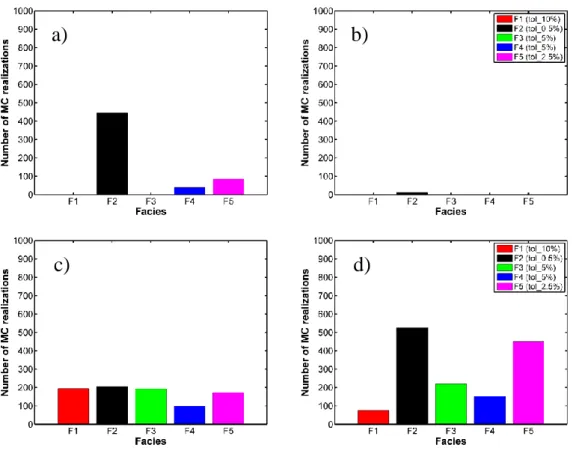
5.3.2. Statistical analysis of SISIM and TPS output volumetric proportions ... 53
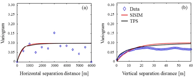
5.3.3. Variogram calculations from output simulations (SISIM and TPS) ... 58
5.3.4. Sample LogK fields for mean (µ) and variance (σ2), from SISIM and TPS ... 60
6. FLOW FIELD SIMULATIONS ... 63
6.1. Stating the problem: modeling details and procedure ... 63
6.1.1. Numerical grid ... 64
6.1.2. Boundary conditions ... 66
6.2. N-S and W-E ensemble average drawdown maps ... 67
6.3. Hydraulic heads’ variance and covariance maps for different degrees of vertical averaging ... 71
6.4. Sample pdf estimation for point and vertically averaged hydraulic heads ... 76
6.5. Sample pdf fitting procedure to Gaussian and α-stable models ... 80
7. DISCUSSION ... 88
7.1. Practical applications ... 88
7.2. Objective and novelty ... 88
7.3. Indicator simulations ... 91
7.3.1. Comparison of SISIM and TPS results ... 92
7.3.2. Providing guidelines ... 93
7.3.3. Consequences of using SISIM and/or TPS ... 95
7.3.4. When should be used one or another? Both? ... 97
7.4. Flow field simulations ... 99
7.4.1. Comparison of SISIM and TPS results ... 100
7.4.2. Providing guidelines ... 107
7.4.2.1. Vulnerability issues... 109
8. CONCLUSIONS ... 110
3
9.1. Publications ... 114
9.2. Dissemination activities ... 115
9.2.1. Conferences and workshops ... 115
9.2.2. Posters at international conferences ... 115
9.2.3. Oral presentations ... 116
9.3. Appendix to Chapter 7 ... 117
4
1. Introduction
The current Ph.D. thesis has been developed under the umbrella of the European Marie Curie ITN (Initial Training Network) IMVUL “Towards improved groundwater vulnerability assessment”.
1.1. Aims
The aim pursued with this work is to improve our current knowledge in numerical modeling applied to hydrogeology, by means of conducting statistical analyses of the outcome of the procedures/workflows adopted and the application of the results to real field case studies.
The project we carried out is mainly focused on the use and comparison of two geostatistical techniques to produce heterogeneous aquifer simulations in order to simulate the flow field induced by a mean hydraulic gradient superimposed to the effect of a pumping well in a real double aquifer system. A posed problem of the kind is relevant to hydrogeology practitioners, especially to those related to groundwater vulnerability and its characterization and/or quantification. The actual system bears at surface level a natural and active springs’ network which is threatened by anthropological activities such as water over abstraction, due to excessive pumping effects for agricultural (mainly) and industrial purposes. We did combine a stochastic approach with the inclusion of real hard data (lithological input from available boreholes) to condition the aforementioned geostatistical simulations. We created a reality-based numerical model to study the impact of the hydrofacies generation scheme and the effect of competing hydraulic stresses over a given environmental target parameter of our
5
choice: h (hydraulic heads). The output of a study of the kind we propose could be used to guide setting thresholds or limits in water abstractions, in order to control hazardous drawdowns that could lead to the drying up of a springs’ network fed by a confined aquifer.
1.2. Objectives
In this dissertation, we perform a numerical Monte Carlo (MC) study based on a geological system whose heterogeneous structure mimics the one associated with an alluvial aquifer system located in northern Italy (Cremona province, Regione Lombardia) where abundant lithological and geological information are available. Our analysis considers a non-uniform flow scenario due to the superimposition of a base non-uniform (in the mean) flow and the action of a pumping well. Field-scale available lithological data are analyzed to characterize prevalent lithotype categories and the associated geological contact rules. The simulation domain is modeled as a composite medium with randomly distributed hydrofacies, each associated with a given hydraulic conductivity. Collections of conditional Monte Carlo realizations of the three-dimensional geomaterials distributions are generated by (i) a classical indicator-based approach (Sequential Indicator simulations, SISIM) and (ii) the Truncated Plurigaussian simulations (TPS) scheme, starting from available data which are employed as conditioning information. Afterwards we performed a statistical analysis (in terms of mean, variance, covariance function and probability distribution) of hydraulic heads as a function of (i) location in the domain and (ii) methodology of geological reconstruction of the system, highlighting the competing effect of the source term and boundary conditions. Since typical head observations are collected within screened boreholes, we explore the extent to which vertically averaging hydraulic heads can retain qualitative and quantitative information on the statistical behavior of point-wise head values.
6
1.3. Structure
The dissertation is organized as follows. We do start framing our research revising the previous scientific contributions by means of a review of the available literature in Chapter 2. Chapter 3 is devoted to illustrate the reader with the current information database related to the real field case study. There we describe the geological setup and present the previous studies/surveys carried out in the area. We point out the relevance of the chosen area in terms of groundwater vulnerability issues drawing the scenario where the numerical analysis is meant to be applied for. A description of the available lithological database is performed. Chapter 4 reports details about the methodology developed and employed. From modifying the available borehole database in order to simplify the naturally high heterogeneity of the hydrofacies system, through recalling some basic geostatistical concepts needed for our study, we introduce the two widely used geostatistical approaches employed to conditionally simulate (to hard data), in a MC framework, the large scale confined aquifer. We describe the hydrofacies simulation stage and the flow field simulations performed by means of the commonly used MODFLOW code. Finally we provide some guidelines on how we treated the output at different stages to allow reproduction of the results, bringing light to the procedure utilized to perform the posterior statistical analysis. Chapter 5 treats in detail the hydrofacies simulations approach adopted in our study while Chapter 6 deals with the description of the aquifer flow field simulations. A thorough discussion upon the obtained results is performed in Chapter 7, both for the geostatistical reconstruction of the aquifer system and the flow simulations. We end up with the major findings and conclusions, along with future work and potential research tracks that can be pursued. Annexes / Appendixes containing publications, dissemination activities and other extra material can be found at the end of this work. Before its end we enclose a list with scientific references.
7
1.4. Originality and principal outcome
The novelty of our study is rooted in the fact of investigating the relative impact of two different conceptualization and simulation techniques to characterize random hydrofacies spatial arrangement on the probabilistic distribution of hydraulic heads in three-dimensional aquifer systems, under non-uniform mean flow conditions of the kind that are associated with large scale field. This analysis is intimately tied to Probabilistic Risk Assessment (PRA) procedures and constitutes one of the steps which can be adopted in modern PRA applications based on the idea of decomposing the full problem (that might comprise several uncertainty sources, including those associated with hydrostratigraphic structure, aquifer recharge, boundary conditions, location and/or pumping/injection rate of wells) into sets of basic events. History matching and inverse modeling are out of our scope in the present study.
Amongst the main findings we would like to highlight that hydraulic heads deduced from TPS-based flow simulations reveal larger variability than their equivalents evaluated by a SISIM-based modeling strategy. This can be seen as a consequence of setting geological contact rules, as considered within a TPS simulation scheme, which can lead to an increased variability in the internal architecture of hydrofacies distributions within a relatively large-scale aquifer model of the kind we consider.
Due to the enhanced degree of variability displayed within the collection of simulations and to the occurrence of long-tailed pdfs, reliance on a TPS scheme produces a broader range of possible drawdown values for the simulated groundwater system. As such, TPS-based results are associated with the most conservative (in terms of extreme values) drawdown estimates which can then be related to a given threshold probability of occurrence in the context of PRA protocols, where the target environmental metric is the piezometric drawdown.
8
2. Literature review
Heterogeneity is embedded in practically all life systems at almost every scale. This assumption also affects/includes geosciences and its related fields/disciplines. In particular we are interested in characterizing the natural heterogeneity that exists in groundwater systems, by means of Geostatistics and numerical simulations, specifically at a field scale. This is one of our objectives in order to improve the current knowledge in numerical modeling of water reservoirs and links to the more general aim of estimation and quantification of groundwater vulnerability in real/natural systems.
We decided to employ widely used and well-known, both by academics and practitioners, geostatistical and numerical tools to simulate a double aquifer system and its associated flow field when a pumping well is acting as a sink/forcing term in the system. The situation just described is compatible with actual field practices like water abstractions for agricultural, industrial or drinking water purposes. These stresses are applied to natural environments which react in turn, mostly having a negative impact on the available water resources and the surrounding natural environments. Sometimes the aforementioned stresses are pushed to certain limits that drive the system into a non-equilibrium state. Since these activities cannot cease due to civil/industrial requirements, a compromise needs to be met in order to protect the resources we are exploiting (and sometimes overexploiting).
What we propose is a stochastic approach conducted at a field scale, involving geostatistical and numerical analyses, in order to compare two methodologies and the joint information we can extract from their outcome. In other words, we compared two well-established geostatistical methods that treat in a different way the heterogeneity embedded in
9
natural systems, and the impact of the geostatistical simulation on the posterior flow field solution (and in particular, on the hydraulic heads). This allowed us estimating low order moment statistics of calculated hydraulic heads in order to forecast which method introduces more variability in the results and/or which method can be useful as a function of the context under study (extreme values analysis, worst case scenario, etc.). From a practical point of view, in stochastic hydrogeology, it is of great importance being able to put thresholds on water abstractions that might lower local/regional hydraulic heads leading towards a real menace to the available groundwater resources.
The present work is focused on the assessment of the impact on hydraulic head statistics of two geostatistically-based methodologies for the stochastic simulation of the spatial arrangement of hydrofacies in field scale aquifer systems. The relevance of an appropriate characterization of the probability distribution of hydraulic heads is critical in the context of Probabilistic Risk Assessment (PRA) procedures which are nowadays considered as viable procedures to estimate the risk associated with catastrophic events in environmental problems (Tartakovsky, 2013 and references therein). Application of PRA to actual settings typically requires the estimate of the probability density function (pdf) of a target Environmental Performance Metric (EPM, a terminology introduced by De Barros et al., 2012).
The study of the relative impact of different conceptualization and simulation techniques to represent random hydrofacies spatial arrangement on the probabilistic distribution of hydraulic heads in three-dimensional aquifer systems under non-uniform mean flow conditions of the kind that is associated with large scale field settings is still lacking. As highlighted above, this analysis is tied to Probabilistic Risk Assessment procedures and constitutes one of the steps which can be adopted in modern PRA applications based on the
10
idea of decomposing the full problem (that might comprise several uncertainty sources, including those associated with hydrostratigraphic structure, aquifer recharge, boundary conditions, location and/or pumping/injection rate of wells) into sets of basic events (e.g., Bolster et al., 2009; Jurado et al., 2012; Tartakovsky, 2013 and references therein).
Here we perform a numerical Monte Carlo study based on a geological system whose heterogeneous structure mimics the one associated with an alluvial aquifer system located in northern Italy, where abundant lithological and geological information are available. Our analysis considers a non-uniform flow scenario due to the superimposition of a base uniform (in the mean) flow and the action of a pumping well. Field-scale available lithological data are analyzed to characterize prevalent lithotype categories and the associated geological contact rules. The simulation domain is modeled as a composite medium with randomly distributed hydrofacies, each associated with a given hydraulic conductivity. Collections of conditional Monte Carlo realizations of the three-dimensional geomaterials distributions are generated by (i) a classical indicator-based approach and (ii) the TPS scheme, starting from available data which are employed as conditioning information. We present a statistical analysis (in terms of mean, variance, covariance function and probability distribution) of hydraulic heads as a function of (i) location in the domain and (ii) methodology of geological reconstruction of the system, highlighting the competing effect of the source term and boundary conditions. Since typical head observations are collected within screened boreholes, we explore the extent to which vertically averaging hydraulic heads can retain qualitative and quantitative information on the statistical behavior of point-wise head values.
11
2.1. Geostatistical simulations
Geostatistics can be roughly defined as the branch of Geology and/or Statistics that deals with the study of phenomena that vary over the spatial dimension. It was developed originally in the context of mining industry, to tackle problems that dealt with the spatial prediction of mineral ore grades. Its general approach led afterwards to its vast application in a wide range of settings across the geographical, geological, atmospheric, environmental, and epidemiological sciences (among others). Geostatistics mainly provides a set of probabilistic tools that help in understanding and modeling the spatial variability of a target variable of interest, bearing in mind the main motivation of predicting unsampled values of the aforementioned variable over areas/volumes where little/scarce information is provided. This process is also (well-) known as interpolation. It is necessary to soar to the work of Daniel Krige and other authors to find the origins of the discipline. They developed methods to calculate/estimate gold and uranium reserves in the Witwatersrand, in South Africa, during the decade of the 1950’s. Their ideas were extended and formalized during the 1960’s by the French statistician Georges Matheron, who coined the term Geostatistics.
The selection of a model through which one can describe the natural heterogeneity of a system is a key point in the analysis of the distribution of groundwater flow (and possibly transport) variables. The model choice strongly depends on the scale of investigation. At the large field scale, geological heterogeneity of sedimentary bodies can be represented and modeled from information on depositional facies distributions. Statistical grid-based sedimentary Facies Reconstruction and Modeling (FRM) methods can be employed to provide consistent representations of facies distribution and are amenable to include conditioning to hard and/or soft data. Falivene et al. (2007) provide an overview of the most widely used deterministic and stochastic FRM methods, including pixel-based methods
12
termed as sequential indicator simulation (SISIM), transition probability schemes (e.g., T-PROGS; Carle, 1999), multiple point simulation (Strebelle, 2002; Zhang et al., 2006; Wu et al. 2008), truncated Gaussian simulation (TGS) and truncated plurigaussian simulation (TPS).
Sequential indicator algorithms are widespread geostatistical simulation techniques that rely on indicator (co-) kriging. These have been applied to different datasets to study the influence of the random distribution of aquifer sedimentological facies on target environmental variables. In this context, Riva et al. (2006) present a synthetic numerical Monte Carlo study aimed at analyzing the relative importance of uncertain facies architecture and hydraulic attributes (hydraulic conductivity and porosity) on the probabilistic distribution of three-dimensional well catchments and time-related capture zones. The authors base their comparative study on a rich database comprising sedimentological and hydrogeological information collected within a shallow alluvial aquifer system. Riva et al. (2008, 2010) adopt the same methodology to interpret the results of a field tracer test performed in the same setting. These authors consider different conceptual models to describe the system heterogeneity, including scenarios where the facies distribution is random and modeled through a SISIM-based technique and the hydraulic properties of each material are either random or deterministically prescribed. Comparisons between the ability of different geostatistical methods to reproduce key features of field-scale aquifer systems have been published in the literature (e.g., Casar-González, 2001; Falivene et al., 2006; Scheibe and Murray, 1998, Dell’Arciprete et al., 2012). Lee et al. (2007) performed a set of Monte Carlo simulations to mimic a pumping test in an alluvial fan aquifer using the sequential Gaussian simulation method and the transition probability indicator simulation. Emery (2004) highlights limitations of SISIM upon examining the conditions under which a set of realizations is consistent with the input parameters.
13
Truncated Gaussian simulation enables one to condition simulations on prior information stemming from various sources while guaranteeing consistency between variogram and cross-variogram of the variables considered. The possibility of using a multiplicity of Gaussian functions to codify hydrofacies extends the potential of TGS and is the cornerstone of TPS (Galli et al., 1994). Later on, Le Loc’h and Galli (1997) extended the aforementioned reference. TPS allows taking into account complex transitions between material types and simulating anisotropic distributions of lithotypes, whereas TGS explicitly considers only sequentially ranked categories. The application of TPS usually aims at (i) assessing the uncertainty associated with the location of the internal boundaries demarcating geomaterials within the domain, and (ii) improving the geological constraints in the characterization of quantitative attributes such as mineral ore grades. TPS is typically employed to simulate geological domains in different contexts, including petroleum reservoirs and mineral deposits, spatial arrangement of hydrofacies in aquifers, or soil types at a catchment scale (e.g., Betzhold and Roth, 2000; Skvortsova et al., 2000; Fontaine and Beucher, 2006; Galli et al., 2006; Emery et al., 2008; Dowd et al., 2007; Mariethoz et al., 2009). More recently, a few publications brought open source codes/suites to use the TPS workflow in standard personal computers (Dowd et al., 2003; Xu et al., 2006 and Emery, 2007). The routines are available as FORTRAN and MATLAB codes.
2.2. Hydraulic head pdfs
In the groundwater literature, the functional format of probability distributions of solute travel/residence times, trajectories and concentrations has been extensively analyzed during the last years (Fiorotto and Caroni, 2002; Bellin and Tonina, 2007; Riva et al., 2008, 2010; Schwede et al., 2008; Enzenhoefer et al., 2012 amongst others). On the other hand, less attention has been devoted to study the probability distribution of hydraulic head (h) in
14
complex groundwater systems and under non-uniform (in the mean) flow conditions. These settings are crucial for the study of the (negative) consequences arising from events associated with the occurrence of h dropping below (or rising above) a given threshold. These basic events are critical for various goal-oriented risk assessment practices including, e.g., the protection of natural springs, ponds or the prevention of damages to underground infrastructures. They all constitute core requirements in the planning of groundwater abstraction procedures or during the designing of protection barriers. In this context, estimates of first and second (conditional or unconditional) statistical moments of h have been largely analyzed by means of analytical (e.g., Guadagnini et al., 2003; Riva and Guadagnini, 2009 and references therein) or numerical (e.g., Guadagnini and Neuman, 1999b; Hernandez et al., 2006) methods for bounded randomly heterogeneous aquifers under the action of pumping. Low-order (statistical) moments (i.e., mean and variance-covariance) of hydraulic heads in unbounded and bounded domains under uniform (in the mean flow) conditions have been investigated, amongst others, by: Dagan (1985), Rubin and Dagan (1988, 1989), Ababou et al. (1989), Dagan (1989), Osnes (1995), Guadagnini and Neuman (1999a, b). Even as these low-order moments have a considerable theoretical and practical interest, they are not directly suitable to PRA protocols where the behavior of the tails of the target variable distribution needs to be identified. This behavior can differ from the one dictated by the classically assumed Gaussian or lognormal distributions and can be influenced by the type of system heterogeneity, hydraulic boundaries and source/sink terms, as we discuss in this work.
Jones (1990) observed the non-Gaussian shape of heads’ pdf close to pumping wells in a two-dimensional confined aquifer where the transmissivity is lognormally distributed and spatially correlated according to an exponential covariance model. Kunstmann and Kastens
15
(2006) modeled an aquifer in Gambach (Germany) under general non-uniform flow conditions as a two-dimensional, block-heterogeneous system, where transmissivity is homogeneous within each of five considered distinct zones. These authors noted that groundwater velocities could be well approximated by lognormal distributions while heads could be best described by long-tailed pdfs (such as the Weibull or the Gamma distributions). Nowak et al. (2008) presented a detailed numerical study centered on the analysis of statistical moments and pdf of heads and velocity components. Their work involved three-dimensional flow through realizations of randomly heterogeneous conductivity fields subject to uniform mean flow conditions. The authors noted that the shape of heads’ pdf is similar to a Gaussian or a Beta distribution at locations which were respectively far or close to the Dirichlet boundaries. The longitudinal discharge components appeared to be well interpreted by a lognormal distribution while their transverse counterparts displayed long tails. Additional studies which are concerned with key statistics of groundwater fluxes under uniform (in the mean) flow conditions include the works of Englert et al. (2006) and Zarlenga et al. (2012).
16
3. Cremona field case study
In this section we describe the Cremona aquifer from a hydrogeological point of view.
3.1. Area under study
3.1.1. Location
The area subject of this study is the territory portion of the Pianura Padana valley bounded to the west and south by the river Adda (which runs North-South) to Crotta d'Adda, where it enters the river Po, and eastward from river Serio, which runs along the North-South direction until Montodine, where it flows into the river Adda.
In the absence of a clear identification of a hydrogeological boundary, the demarcation of the northern limit was evaluated in a manner consistent with other studies conducted in the aforementioned region. In particular, it was adopted the same northern boundary identified in a thesis project developed at the Politecnico di Milano by Rametta, (2008). That is located along the northern boundary running parallel to the coordinate Gauss-Boaga 5060000 North. The limits described above identify an area of approximately 785 km2. This system will be identified later in terms of “the large scale model”. Figure 3.1.1.1
17
Figure 3.1.1.1: Sketch of the area from which sedimentological data are extracted including the location of (a) Regione Lombardia in Italy, (b) the large scale aquifer system studied by Bianchi Janetti et al. (2011) along with the sample area marked with a black rectangle, and (c) sub-domain where conditional lithofacies simulations are performed (delimited by a black rectangle) together with the local borehole network.
In this region was also identified a sample area. The location of it is shown schematically in Figure 3.1.1.1. The choice was made on the basis of considerable strategic importance of the area under consideration, due mainly to the following factors:
Presence of numerous springs that feed a series of significant spring tails.
Important interaction between surface water and groundwater. The contemporary analysis of the effect of major springs, a dense network of surface channels and pumping wells (which are used either for drinking water or irrigation purposes) requires modeling of a wide range of physical processes for describing the distribution of water flows in the area.
These elements make the problem interesting from a scientific point of view, because it requires the adoption of sophisticated modeling techniques. The problem is also relevant from an operational point of view, since the presence of interactions between different physical processes enhances the representativeness of the region to characterize the
18
phenomena that takes place in the whole range of fountains that develops in the West (eastern Pianura Padana).
3.1.2. Previous studies
Hydrogeological studies conducted by Maione et al. (1991) and Gandolfi et al. (2007) investigated, respectively, the portion of the province of Bergamo in the south of the Alps Orobie and the entire province of Cremona. These studies have provided an important source of data and a valuable source of prior knowledge of the area investigated.
The area surveyed by Maione et al. (1991) is located between the rivers Adda and Serio and bounded by the Alps and the northern outcrop line of fountains. The authors proposed a geological model which identifies two distinct aquifers: a shallow phreatic aquifer and a deep artesian aquifer, which flows beneath the surface without significant interaction with the former.
The model proposed by Gandolfi et al. (2007) which covers the entire province of Cremona, is bordered in the West by the river Adda, on the East by the Oglio river and in the South by the river Po. In the North, since there is a lack of natural water boundary that can be adopted as a closure model, was chosen the northern boundary along a line joining the rivers Adda and Oglio at a distance of several kilometers North of the administrative boundary of the province of Cremona. The conceptual model of the aquifer system shows a double system of groundwater flow with:
A surface portion characterized generally by high transmissivity and large flow values supported by the surface trade with the hydrographical network. Recharge is due to infiltration from rainfall and water used for irrigation.
19
A deeper portion characterized by a complex succession of geological bodies with different conductivities, which are essentially governed by the flow of water withdrawals for drinking water supply. Its flow values are well below the ones transiting the upper portion.
3.1.3. Hydrogeological structure
The available literature research and the collection of stratigraphic data were initially extended to the provinces of Bergamo and Cremona. At a later stage, attention was focused on the portion of land bounded by the paths of the rivers Adda and Serio.
The preliminary conceptual geological model of the area under investigation was constructed on the basis of the following information and documents:
Maione et al. (1991): drawn from the study were 218 stratigraphic columns located in the provinces of Bergamo and Cremona and 15 reconstructed lithostratigraphic sections.
Provincia di Cremona – Atlante Ambientale: in the study were used 464 stratigraphic columns located within the province of Cremona.
Consorzio della Media Pianura Bergamasca (CMPB): we used 14 stratigraphic columns.
Beretta et al. (1992): the study contains 29 reconstructed lithostratigraphic sections from the province of Cremona.
The analysis of the sections can schematically identify, within the territory examined, the presence of two overlapping aquifers within the Quaternary alluvial sequence of the Padano sedimentary basin filling. This fact allows considering two different aquifers.
20
Phreatic aquifer. It is located in the coarse clastic deposits ranging between the ground level and a clay level that is characterized by certain continuity at the investigation scale. The roof of the body with low hydraulic conductivity, named by Maione et al. (1991) “A horizon”, coincides with the clay level in the high plain which is present in the most superficial fluvio-glacial Valtellina complex (which separates the polygenic strain from the underlying calcareous strain). In the lowlands the delineation of the A horizon is more uncertain. In general it is represented by a clay layer being within the same alluvial deposit, following the criteria of Maione et al. (1991).
The superficial thickness consists of thick clastic continental deposits belonging to different sedimentary cycles that appertain to diverse geological periods. Nevertheless, they display a lateral continuity between them in terms of the hydraulic conductivity parameter. Within these, stand out the following:
Polygenic conglomerate (fluvio-glacial Mindel) in the high plains.
Fluvio-glacial gravels and sands (RISS-Wurm) that form the lowlands and the filling of the erosion furrows in the polygenic conglomerate.
Recent alluvial gravels and sands deposited by rivers that cross the plain.
In the northern line of Canonica d'Adda - Ghisalba prevail the conglomeratic deposits, while in the southern portion dominate loose gravel and sand deposits. Within the aquifer thickness are intercalated layers of clay with variable planar/lateral continuity. Due to this fact, the aquifer may shift from ground conditions to local conditions of semi-confinement. The thickness of this aquifer ranges from 40 m to 80 m, along the main anisotropic direction of the system (North-South).
21
Confined aquifer. Below the level of clay which forms the basis of the aquifer water table surface, there is a succession formed by alternating coarse clastic sediments and clays whose degree of continuity and relative thickness of the deposits (displaying different grain size) is very variable. Inside the porous and/or fractured layers, confined by other layers of fine-grained sediments, artesian aquifers are based. The base of the sequence described, called “B horizon” by Maione et al. (1991), consists of clay minerals with occasional inter-bedded (predominantly sandy) lithotypes.
The reconstructed sections show that the geological system has artesian aquifers of variable thickness depending on the geometry of the substrate. It is a range characterized by a significant thickness (170 m to 200 m) controlled by the alignment Osio Sopra-Osio Sotto, Levate-Verdellino, Comun Nuovo-Urgnano and in the area of Cologno al Serio. This thickening represents the filling of a morphological-tectonic graben. Going southwards of the identified structural sections, aligned with the SW-NE direction in accordance with the alignment Ghisalba-Treviglio, the complex artesian aquifer tends to decrease significantly (up to 30 - 40 m) with an increase in percentage of the clay-rich levels over the porous ones.
In the plain portion of the territory under study, the information that can be derived from stratigraphic data allows to outline the characteristics of the subsurface by means of the following lithostratigraphic units:
Predominant gravel-sandy deposits whose continuity is interrupted by locally inter-bedded silt-clay lithotypes.
Alternation of gravelly-sandy and silt-clay lithotypes. Predominant silty-clay deposits with occasional sand. Mainly fine deposits, sometimes of the silty-sandy type.
22
3.1.4. Wells / piezometers
Information concerning the presence of wells/piezometers comes from the following sources:
Regione Lombardia: Programma di Tutela e Uso delle Acque – PTUA.
Agenzia Regionale per la Protezione dell’Ambiente Lombardia - ARPA Lombardia.
Consorzio di Bonifica della Media Pianura Bergamasca – CMPB.
Piezometric monitoring of the aquifer system in the region under consideration, can be done using information from a set of 761 observation wells. It is worthy to point out that a number of wells outside the large-scale model area were taken into account. This choice aims at achieving greater consistency in order to track the reference piezometric maps, particularly on the rivers which shape the limits of the superficial area influenced by the groundwater flow model.
Information on the measurements of the land surface at the individual wells is associated by means of using heterogeneous techniques. Among them, are included:
GPS measurements.
Interpolation from the base of the Regional Technical Cartography. Topographic lines.
Unfortunately, it was not possible to trace the detailed description of the origin of these values for each well. A first empirical test of the reliability of the allowances provided, was determined by estimating the values of the land surface at the wells of interest from the Digital Elevation Model DTM40.
23
The reliability of the data reported is of fundamental importance for a proper definition of the piezometric level in the region. In fact, the measure monitored at all points of observation is not the piezometric level, but rather the depth to the water table with respect to the ground level. The piezometric level has been rebuilt, for each well/piezometer, as the difference between the values of water table depth and the land surface.
The water table depth data from ARPA, registered monthly or bimonthly, covers a time span between 1999 and 2006, while the database provided by the CMPB covers a longer period which goes from 1989 to 2007. The measurement campaigns conducted by CMPB are carried monthly or every two months. The water table depth data recorded by the Politecnico di Milano (and reported within the PTUA) refers to three different surveys conducted in April 1994, November 1996 and March 2003.
Figure 3.1.4.1: Location of the wells in which the piezometric level is currently monitored (Guadagnini, L. et al., 2008).
24
3.1.5. Springs
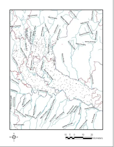
The intricate drainage network that characterizes the study area is largely fed by a great number of springs, typical hydrogeological items of the northern side of the Pianura Padana. Within the area delimited by the large-scale model there are a total of 161 spring heads (depicted in Figure 3.1.5.1). The location of the aforementioned springs is derived from the following sources:
Protection Program and Water Uses, Lombardia region (2006). www.atlanteambientale.it, province of Cremona.
Figure 3.1.5.1: Location of the spring heads (Guadagnini, L. et al., 2008).
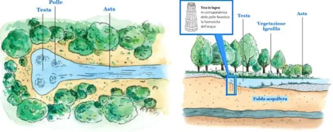
The typical morphology of these hydrogeological structures is depicted in the following images (Figure 3.1.5.2).
25
While the two top pictures represent the typical planar section (top left) and vertical cross-section (top right) of a spring, the bottom diagram illustrates the Pianura Padana system from the highest area located in the North (Alps) to its distal zones. It can be noted here that, as it is observable through our borehole database, exists a transition from coarser materials in the northern boundary towards finer materials (when we approach the distal parts of the alluvial system).
Figure 3.1.5.2 : Source: http://www.comune.capralba.gov.it/parco/territorio/fascia/index.aspx#/-1/, http://www.cooperativadelsole.it/?p=446.
26
3.2. Reference information database
Implementing a flow model within a real aquifer system requires the structuring of an information database that should contain a complete set of data necessary to understand, with the greatest degree of detail possible, the geological architecture of the porous medium and the hydrological processes that govern the flow field in the area under study. This database should be structured in an organic and functional way, to:
Allow rapid access to the information of interest.
Ensure the ability to update quickly and effectively the data collection. Guarantee the ability to interact with the mathematically formulated model.
A rough outline that could describe how the reference information database was implemented can be divided into the following stages:
Collection of raw data from the different agencies responsible for monitoring the quantities of interest.
Data selection for the region studied.
Analysis and processing of data in order to evaluate its significance at different temporal and spatial scales.
Structuring the reference information base.
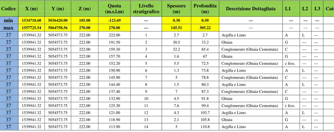
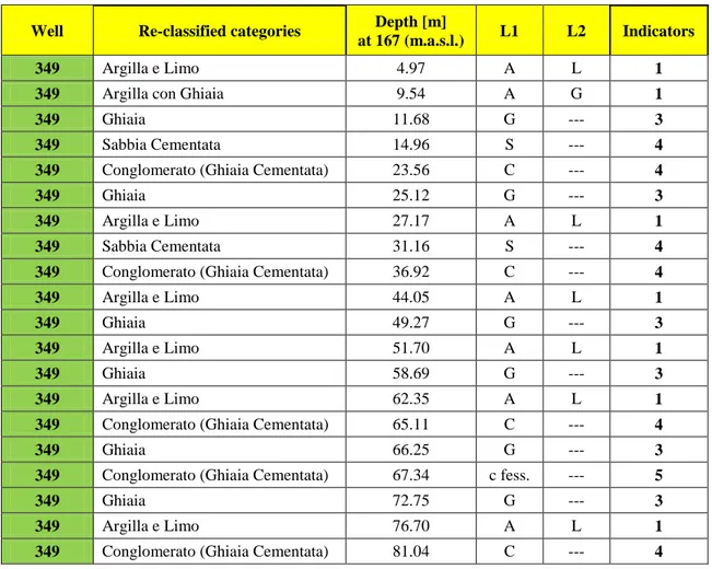
In Table 3.2.1 we present an extract of the already re-worked lithological database. The information contained in the table below is compartmented in columns displaying, amongst other fields: the well code (corresponding to the original database and map vertical cross-sections); the three-dimensional UTM coordinates; identified strata thickness; its relative depth expressed in m.a.s.l (meters above sea level); the detailed lithological description and its indicator category.
27
Table 3.2.1: This database sample displays the rich geological data record build up aiming to obtain the necessary hard data for our simulation phase process, i.e. the variogram analysis and the a posteriori geostatistical (conditional) simulations.
Codice X (m) Y (m) Z (m) Quota (m.s.l.m) Livello stratigrafico Spessore (m) Profondita
(m) Descrizione Dettagliata L1 L2 L3 Categoria
min 1534718.60 5036420.00 105.00 -123.69 --- 0.30 0.50 --- --- --- --- ---
max 1557725.54 5064758.56 270.00 270.00 --- 145.51 305.22 --- --- --- --- ---
37 1539941.32 5054573.75 222.00 222.00 1 2.7 2.7 Argilla e Limo A L --- 1
37 1539941.32 5054573.75 222.00 191.50 2 30.5 33.2 Ghiaia G --- --- 3
37 1539941.32 5054573.75 222.00 159.30 3 32.2 65.4 Conglomerato (Ghiaia Cementata) C --- --- 4
37 1539941.32 5054573.75 222.00 157.70 4 1.6 67 Ghiaia G --- --- 3
37 1539941.32 5054573.75 222.00 152.20 5 5.5 72.5 Conglomerato (Ghiaia Cementata) c fess. --- --- 5
37 1539941.32 5054573.75 222.00 150.90 6 1.3 73.8 Argilla e Limo A L --- 1
37 1539941.32 5054573.75 222.00 145.90 7 5 78.8 Conglomerato (Ghiaia Cementata) C --- --- 4
37 1539941.32 5054573.75 222.00 144.40 8 1.5 80.3 Argilla e Limo A L --- 1
37 1539941.32 5054573.75 222.00 137.40 9 7 87.3 Conglomerato (Ghiaia Cementata) C --- --- 4
37 1539941.32 5054573.75 222.00 132.90 10 4.5 91.8 Ghiaia G --- --- 3
37 1539941.32 5054573.75 222.00 125.30 11 7.6 99.4 Conglomerato (Ghiaia Cementata) c fess. --- --- 5
37 1539941.32 5054573.75 222.00 121.00 12 4.3 103.7 Argilla e Limo A L --- 1
37 1539941.32 5054573.75 222.00 118.90 13 2.1 105.8 Ghiaia G --- --- 3
28
The total drilled depth information used in the area under study is slightly over 13.5 km (data belongs to the CMPB). For our purpose of quantifying the existing volumetric proportions of the five re-classified lithotypes, and therefore finding a hint to establish the final indicator values, we used the information coming from a bulk set of 144 wells. We chose to keep constant the indicator volumetric proportions across the three-dimensional space. We know that it is not a 100% realistic assumption but it helps to keep simpler, yet valid, the problem under analysis.
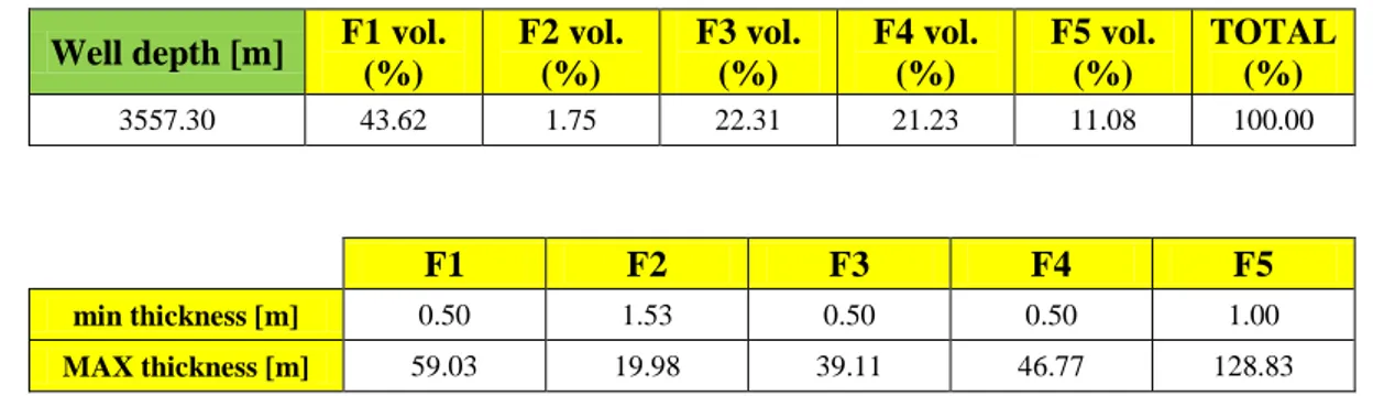
We did carry a statistical analysis over some key features including the ones presented in Table 3.2.2, in order to bring light to the modeling problem and be able to find proper constraints for solving the geostatistical and the flow field simulations. For instance, knowing the minimum well depth, its maximum and the mean, allowed us to set the boundaries in the vertical direction for our numerical domain. We used, for our numerical simulations, the vertical geological cross-sections along the N-S direction (namely S3, S4 and S5) as detailed in the study from Guadagnini, L. et al. (2008). Along the W-E direction we used the S10 and S11. The total borehole depth used as conditioning data adds up to almost 3.6 km, i.e. a whole set of 35 wells. The minimum thickness recorded in the borehole dataset is 0.5 meters. We did use this information to further discretize our remaining hard data.
Well depth [m] F1 vol. (%) F2 vol. (%) F3 vol. (%) F4 vol. (%) F5 vol. (%) TOTAL (%) 3557.30 43.62 1.75 22.31 21.23 11.08 100.00 F1 F2 F3 F4 F5 min thickness [m] 0.50 1.53 0.50 0.50 1.00 MAX thickness [m] 59.03 19.98 39.11 46.77 128.83
Table 3.2.2: The top table displays the total drilled depth used to condition the numerical simulations and estimate the volumetric facies proportions (kept constant across the full domain). The bottom table shows the minimum and maximum thicknesses for every hydrofacies expressed in meters [m].
29
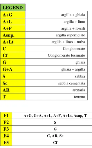
Table 3.2.3: The top left table represent the main lithotype classes found in the sample area under study, while the bottom left table displays the re-categorized hydrofacies and the original categories that were included in each one. The top right table is presented to show a key finding that helped to establish the lithotype rule for the Truncated Plurigaussian simulations. There we illustrate (in percentage values) the existing 456 transitions between the different geomaterials. This has nothing to do with probability transitions. We wanted to investigate qualitatively and quantify the amount of times a facies appears next to the other remaining facies.
LEGEND
A+G argilla + ghiaia
A+L argilla + limo
A+F argilla + fossili
Asup. argilla superficiale
A+Lt argilla + limo + turba
C Conglomerate
Cf Conglomerate fessurato
G ghiaia
G+A ghiaia + argilla
S sabbia Sc sabbia cementata AR arenaria T terreno TOTAL F1-F1 F1-F2 F1-F3 F1-F4 F1-F5 Transitions 10.53 1.97 22.37 26.10 11.62 456.00 F2-F2 F2-F3 F2-F4 F2-F5 Check (%) 0.00 1.10 0.66 0.00 100.00 F3-F3 F3-F4 F3-F5 1.32 14.91 3.51 F4-F4 F4-F5 2.19 3.51 F5-F5 0.22
F1 A+G, G+A, A+L, A+F, A+Lt, Asup, T
F2 S
F3 G
F4 C, AR, Sc
30
3.3. Regional vulnerabilities
In the Cremona region the pollutants are not only the most worrying issue. Thanks to the springs’ existence, a rich environment is developed on the ground surface. All the activities that take place surrounding the springs’ area commit an overexploitation of the aquifers in the zone under study. We refer mainly to agricultural practices, water pumping for drinking purposes and industrial use, etc. Those actions produce non-equilibrium in the system, provoking the decrease in the water level in the springs and their influence zone.
3.4. Final remark
We would like to point out some choices that we made at this stage and that affect the latter steps of our research.
The restructured geological database containing the borehole information from different sources allowed us to estimate the volumetric proportions of the final five regrouped hydrofacies. Not only that, we could infer the crucial lithotype rule needed to run the Truncated Plurigaussian simulations scheme. In addition, we determined (after consulting surface lithological maps corresponding to the area under study) the main anisotropy directions (along the N-S, W-E and vertical) and characteristic lengths of the geological structures. As in the vast majority of studies of this kind, our available vertical hard data resolution is much higher than its horizontal counterpart.
We decided to reduce the complex heterogeneity embedded in our natural groundwater system by means of reclassifying the existent lithotypes into five hydrogeologically meaningful hydrofacies. We chose to keep the problem simple by setting stationary hydraulic conductivity values in the aforementioned indicator lithotypes.
31
4. Methodology
In the following we focus on the workflow we employed to pursue the goals stated in the introduction of this dissertation.
4.1. Modifying the geological database
We introduced the actual geological database in Chapter 3, in order to show where the conditioning data for our geostatistical simulations comes from. As previously stated we got a few tenths of borehole records that gave us a hint of the inherent highly heterogeneous nature of the geological materials found in the area under study. To be able to tackle this extra (natural) complexity in an efficient computational way, and in order to get results in a limited amount of time, we decided to re-categorize the existent geological database. We proceeded as follows:
LEGEND
A+G argilla + ghiaia
A+L argilla + limo
A+F argilla + fossili
Asup. argilla superficiale A+Lt argilla + limo + turba
C conglomerato
Cf conglomerato fessurato
G ghiaia
G+A ghiaia + argilla
S sabbia
Sc sabbia cementata
AR arenaria
T terreno
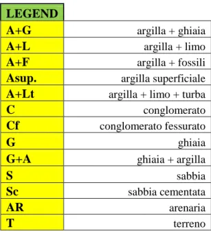
Table 4.1.1: Original lithotypes found in the area under study (left) and the re-classified categories (right).
F1 A+G, G+A, A+L, A+F, A+Lt,
Asup, T
F2 S
F3 G
F4 C, AR, Sc
32
Therefore, by reducing the original lithological classes resulting from previous surveys, we simplified the original problem and improved its computational tractability (in terms of computing effort and time). The new categories or indicators were described as:
F1: fine materials. F2: sands.
F3: gravels.
F4: conglomerates.
F5: fractured conglomerates.
As a way of computing the final volumetric proportions for each indicator, to be used as an input in the geostatistical simulations, we took the newly reclassified values for the different vertical (N-S and W-E) cross-sections and computed the corresponding percentages. The results were the following:
Well depth [m] F1 [%] F2 [%] F3 [%] F4 [%] F5 [%] TOTAL [%]
3557.30 43.62 1.75 22.31 21.23 11.08 100.00
Table 4.1.2: Total borehole depth and estimated volumetric proportions from hard data source.
Initially we were tempted to remove the geomaterial indicator F2 (corresponding to the sandy materials found in the system) due to its low contribution to the final volumetric proportions percentage. Finally we decided to keep it as it was and analyze the impact on the final geostatistical simulations. By keeping the hydrofacies class F2 not only we preserved in a better way the original heterogeneity inherent to the double aquifer groundwater system, but we were able to study the impact on the flow field simulations of a less representative facies. This was possible because we decided to embed into every geomaterial category a steady value of the hydraulic conductivity (K) for each indicator class, i.e. a constant (in time) value of K.
33
We do contemplate the possibility of carrying on with the idea of suppressing the F2 hydrofacies in future studies, derived from the current research project.
4.2. Recalling geostatistical concepts
There exist various basic manuals about Geostatistics either for beginners and practitioners in industry not familiar with the field (Clark, 1979), being mainly focused on the mining industry. Kitanidis (1997) presents an introduction to Geostatistics along with some applications in hydrogeology. “An introduction to applied Geostatistics” is probably the most complete of those references (Isaaks and Srivastava, 1990).
Here we are not interested in delivering a complete geostatistical introduction, since they already exist, but we would rather make explicit which concepts derived/coming from Geostatistics we used for our research work. We used the term Geostatistics in the European sense of the “Theory of the Regionalized Variables” developed by G. Matheron and co-workers at Fontainebleau (1970’s). We made use of the simplest function that characterizes any geostatistical study: the semivariogram. The definition of a semivariogram (γ) arises out of the notion of continuity and relationship due to position. It is a graph (and/or formula) describing the expected difference in value between pairs of samples (bearing a target property of interest) with a given relative orientation. In the following we present its mathematical expression:
γ
Where n are the sample pairs, g are the functions (properties under study) and h is the fixed distance between the sampled positions. In our study we mostly dealt with vertical and horizontal (omni-directional) indicator semivariograms computed from the available conditioning indicator data.
34
4.3. Indicator variogram calculation
Before going through calculating the indicator variograms, we did need to generate further conditioning data by refining (along the vertical direction) the available indicator values. The information contained in the geological database spreadsheet, as usual in borehole/core interpretation, made explicit where the appearance of a given lithotype started/ended. We performed that a priori step in seeking an improvement of the subsequent semivariogram analysis by introducing further more points in the variogram estimation. In order to achieve this, we used an existing in-house built FORTRAN routine (named STRAT). The aforementioned routine performed a data refinement along the vertical by, namely, replicating the available data points every 0.5 meters (when necessary). That generated quite a decent amount of conditioning data, sufficient to accept as valid the posterior results. In any case it is worthy to note that as in almost geostatistical study, the information/resolution obtained along the vertical direction was much higher than that along the horizontal plane. This fact will inevitably condition our results but it is unavoidable from a technical point of view, since it depends on the available data that we have used from previous field studies/surveys. This is a common drawback faced by practitioners of all kind, but does not invalidate the results obtained as long as it is recognized and accepted as a limitation of the approach. In fact, this might lead to inaccurate results, introducing further uncertainty on the final outcome.
For the statistical analysis that we wanted to carry out we needed to compute the vertical and horizontal indicator semivariograms. That was made with the purpose of estimating the ranges (and correlation lengths) of the hydrofacies semivariogram functions. The resulting variogram ranges estimated at this step will act as input information for the geostatistical simulations along with the volumetric proportions estimated previously. We
35
departed from our modified (extended) indicator conditioning dataset. We did use the available computational tools provided for this purpose by the GSLIB manual (program gamv, Deutsch and Journel, 1997). We did perform various types of variogram estimations (mainly omni-directional and along the main anisotropy directions). Those calculations were supported by the available geological information coming from previous studies and superficial lithological maps. We found and determined that the main anisotropy directions were along the N-S, W-E and the vertical direction. Finally we only considered, for posterior fitting with an exponential variogram model, horizontal omni-directional and vertical variograms.
An exponential semivariogram model was chosen (after performing a RSME analysis) for fitting the directional semivariograms. For the purpose of this rather simple data treatment (even though the dataset was pretty vast) and its statistical analysis, we employed common available software packages (such as text and spreadsheet editors).
4.4. SISIM vs TPS (and the geostatistical simulations)
Among the vast range of FRM methods, following the classification in Falivene et al. (2007), we decided to employ 2 different well-known and widely-spread geostatistical indicator pixel-based methods. Those allowed us to compare the effect of the embedded geological heterogeneity in the simulations and the posterior effect on the hydraulic head pdfs, after solving the flow field problem in a multi-realization context. Pixel-based methods work assigning a facies to grid cells according to the facies occurrence pdf, which is computed for each grid cell. These methods allow direct conditioning by hard and/or soft data. Categorical or indicator methods are based on transforming each facies category to a new property, defined as the occurrence probability of the facies, and building the pdf at each
36
grid cell as the combination of the reconstruction or modeling of these new properties (e.g. Journel and Alabert, 1989).
A number N = 1000 of three-dimensional realizations of hydrofacies distributions were generated with TPS and SISIM schemes. Indicator-based conditional simulations are performed via the software SISIM (Deutsch and Journel, 1997). TPS simulations are based on the algorithms and codes presented by Xu et al. (2006) and Emery (2007). This number has been found sufficient to support the validity/correctness of our analyses/work (results regarding this can be found in Chapter 5). For the purpose of our analysis and for reason related to computational costs, the numerical simulations are performed within a model domain whose extent corresponds to the sub-domain identified in Figure 3.1.1.1. The estimated computational effort, in terms of time has been approximately 2 weeks.
At this point we would like to emphasize that we carried out our simulations at a field scale, since the available borehole database allowed for this kind of analysis. The lithological and geological information available in this region were employed as conditioning data for our aquifer system model. The Cartesian grid adopted for the hydrofacies simulations comprises 74 × 86 elements, respectively along the N–S (y) and W–E (x) directions. The grid spacing is set to Δx Δy = 50 m, resulting in a simulation domain with a planar extent of 3700 × 4300 m2. Since one of the objectives of this study is to analyze the way the vertical variability of hydraulic heads is impacted by facies distribution, boundary conditions and/or source terms without considering the effect of the particular geometry of the bottom of the aquifer, we adopt in the following a constant thickness B = 100 m which is representative of an average width of the system in the area. We discretize B into 50 layers of uniform thickness Δz = 2 m for the purpose of our computations. Therefore the total amount of nodes was 74 × 86 × 51, adding up to a total of 324,564 cells.