1
Is it the way you live or the job you have?
Health effects of lifestyles and working conditions
Elena Cottini* and Paolo Ghinetti**
Abstract: This paper investigates the role of lifestyles (smoking, drinking and obesity) and
working conditions (physical hazards, no support from colleagues, job worries and repetitive work) on health. Three alternative systems of simultaneous multivariate probit equations are estimated, one for each health measure: an indicator of self-assessed health, an indicator of physical health, and an indicator of work-related mental health problems, using Danish data for 2000 and 2005. We find that while lifestyles are significant determinants of self-assessed health, they play a minor role for our indicators of physical health and mental health. The effect of lifestyles seems to be dominated by the effect of adverse working conditions, which significantly worsen health. This result is robust for all health dimensions considered.
* Dipartimento di Economia e Finanza, Università Cattolica del S. Cuore, via Necchi 5, 20123 Milano, Italy
email:[email protected]. and Centre for Corporate Performance, Copenaghen Business School, Porcelænshaven 18A/B, 2000 Frederiksberg, Denmark.
** Corresponding author. Dipartimento di Studi per l’Economia e l’Impresa, Università del
2 1. Introduction
An individual’s health is affected by several factors related to both work and non-work activities. Among the latter, good lifestyles have attracted growing attention. Unhealthy behaviour – smoking, heavy drinking, bad eating habits, physical inactivity – and related risk factors are key determinants of major preventable diseases, with high economic and social costs. According to WHO estimates, up to 80% of cases of coronary heart disease, 90% of type 2 diabetes cases, and one-third of cancers can be avoided by adopting healthier lifestyles and quitting smoking (World Health Organisation, 2008).
Among work-related activities, growing attention is paid to how health and emerging risks such as psychosocial working conditions are actually connected at the workplace level. For example, the European Commission has recognised job quality as a key ingredient of the European Employment Strategy (EU, 2001). New sources of health stressors are gaining importance. The period of rapid transformation in the organisation of the production system has promoted a shift from manual occupations to others with a prevalence of soft and intellectual tasks. As a result, the traditional sources of adverse physical working conditions are declining, whereas the share of workers subject to psychosocial job stressors is increasing (Cappelli et al., 1997; OECD, 2008). More research on these issues is important because inadequate working conditions negatively affect health, with costly consequences both for individuals and for the society at large. The social costs of mental health have been estimated to be as high as 3 to 4% of GDP in the European Union (International Labour Organization).
This paper contributes to the literature on the determinants of employee health in two respects. First, we consider the joint effect of lifestyles and work conditions and we also account for their correlation through unobservables. This is important to gauging their genuine health effect which otherwise would be biased by omitted variables. Although the relevance of accounting simultaneously for both aspects seems apparent, it has been widely neglected in the literature. Second, we expand the analysis by considering physical and mental health in addition to a standard measure of self-assessed health. This is important to account for the multidimensional nature of health and to provide additional insight into the complex interplay between risky behaviour, hazardous work conditions and specific health indicators. Evidence on that may provide insights into how to limit work- and
non-work-3 related causes of health decline.
For this purpose we use a unique dataset for Denmark obtained matching the 2000 and 2005 waves of the Danish Work Environment Cohort Study (DWECS) with administrative data from the Statistics Denmark Integrated Labour Market Database (IDA). The resulting dataset provides information on all our dimensions of interest: lifestyles, working conditions and health outcomes. From a policy perspective, Denmark is an interesting country: in recent years the European recommendations in terms of health and safety at work have been implemented by the National Working Environment Authority through a set of guidelines to improve working conditions and screen enterprises in a systematic manner.
Our findings from simple probits show that bad lifestyles and adverse working conditions have a negative association with self-assessed health, physical health and mental health indicators. However, multivariate probits – which account for the endogeneity of working conditions and lifestyles – show that working conditions always play a substantial role in any health measure. On the contrary, a modest net impact is found for lifestyles on physical health and mental health, while effects are maintained on self-assessed health.
The remainder of the paper is organised as follows. In Section 2 we review the relevant literature, while the data are overviewed in Section 3. In Section 4 we present our empirical models, and in Section 5 we present the main results. Section 6 concludes.
2. Related literature
The relationship between lifestyles and health has received considerable attention from epidemiologists (among others, Breslow, 1999; Hu et al., 2005; Patja et al., 2005) and in the areas of medicine and occupational health (Netterstrøm et al., 1991; Hellerstedt and Jeffery, 1997; Otten et al., 1999; Siegrist and Rödel, 2006; Borg and Kristensen, 2000). In economic terms, individual's health is typically treated as a multifaceted good with both consumption and capital features, which are produced over time by individual choices and depend on environmental determinants (Contoyannis and Jones, 2004). In particular, we may think of health as affected by both work-related and non-work-related determinants. Given the multidimensional nature of health, Loprest et al. (1995) stress that, together with general health measures, more specific health dimensions, maybe related to specific
4 symptoms, should also be investigated.
Within economics, Kenkel (1995) pioneered the analysis of the role of non-work-related determinants for health production. He finds that health is significantly affected by several lifestyle choices such as diet, smoking, exercise, alcohol consumption, good sleep, weight (relative to height) and stress. Other studies have focused on single behaviours such as smoking (see, e.g., Blaylock and Blisard, 1992; Mully and Portney, 1990) or have examined interactions between lifestyle choices (see, e.g., Hu et al., 1995).
Balia and Jones (2008) investigate the contribution of lifestyles to socioeconomic inequality in premature mortality in Great Britain. They use a multivariate probit approach to estimate a recursive system for mortality, morbidity and lifestyles. Results show that, once allowing for endogeneity, lifestyles contribute strongly to inequality in mortality, reducing the direct role of socioeconomic status.
Contoyannis and Jones (2004) use panel data from the Health and Lifestyle Survey conducted in the United Kingdom in 1984 and 1991 to estimate the structural parameters of a health production function, together with the reduced forms for six lifestyle equations, by multivariate probits for discrete lifestyles and self-assessed health. They find a reduction in the influence of socioeconomic characteristics on health once lifestyles are included in the analysis. In particular, sleeping well, exercising, and not smoking in 1984 have dramatic positive effects on the probability of reporting excellent or good health in 1991. Moreover, these effects are larger once the endogeneity of lifestyles is accounted for. We extend their framework by including adverse working conditions (together with lifestyles) and two additional health dimensions.
On the work-related variables’ side, Robone et al. (2011) use BHPS data to analyse whether health is hampered by adverse working and contractual conditions. They distinguish between self-assessed health and psychological well-being. The working conditions considered are shift work, overtime, being a union member, supervision and job satisfaction, which are only proxies of the more accurate conceptual categories developed by the literature. They find that being unsatisfied with working hours is negatively related to health, especially in the case of part-time jobs. Having low expectations about future career advancements reduces the health of temporary workers.
5
Spain to detect a causal relationship between the work environment and general versus work-related self-assessed health. Their proxy for working conditions is a single variable for individual satisfaction with the work environment. Moreover, the authors cannot distinguish between mental and physical health. In this context, a separate analysis of the determinants of physical and mental health seems particularly relevant, especially for policy purposes.
A series of studies analyse the link between working conditions and different dimensions of health using the European Working Conditions Survey. Overall they show that adverse working conditions, in terms of psychological job demands and physical hazards, are strongly associated with workers' mental health, supporting the perception that adverse working conditions may harm workers' mental health (Cottini and Lucifora, 2013; Cottini, 2012, among others).
Borg and Kristensen (2000) use the 1990 and 1995 waves from the Danish Work Environment Cohort Study to describe differences in the work environment and lifestyle factors between social classes in Denmark and to investigate if these factors explain social class differences in terms of changes in self-rated health. The authors construct seven indicators describing psychosocial conditions, four scales of physical hazards and two of lifestyles. They find a higher prevalence of repetitive work, low skill discretion, low influence at work, high job insecurity and physical hazards in the lower social classes. High psychological demands and conflicts at work were more prevalent in the higher social classes. With regard to lifestyles, they found that obese people and smokers are more prevalent among the lower classes.
They use the same survey as us but we go about things differently from them, first, by estimating a richer and flexible empirical model which takes advantage of the information at the individual level to model the endogeneity of lifestyle and working conditions. Second, we distinguish between self-assessed, physical and mental health. Third, we focus on a narrower set of working conditions, due to limits imposed by data availability and empirical tractability.
3. Data and variables
6
First is a panel collected every 5 years by the Institute for Occupational Health (AMI) and the Danish Work Environment Cohort Study (DWECS). The questionnaire contains several details about the work environment as well as occupational, health and lifestyle information. For the purpose of this paper, we use the 2000 and 2005 waves since these are the only two for which we can define a wider and comparable set of health outcomes.
Second, we use Statistics Denmark Integrated Labour Market Database (IDA), which includes the Danish population of individual and establishment administrative records together with background characteristics. Danish administrative registers record individual annual earnings as well as demographic and firm characteristics. Even though IDA comprises the whole population of Danish firms and workers, the match with DWECS produces 3,000 observations for each wave.
We measure health in three different ways. The first is an indicator of self-assessed health (SAH).1 Respondents were asked to rank their health status out of five categories ranging from very good to very poor (the question asked is: “How will you overall evaluate your health: 1. Very good, 2. Good, 3. Fair, 4. Poor, 5. Very poor”). We transformed the categorical indicator of SAH into a binary variable that takes the value 1 if perceived health is excellent or good, and 0 if it is fair or poor. This is a general measure of individuals’ health and is subject to well-known conceptual problems. However, it represents one of the most used indicators in the literature (see Datta Gupta and Kristensen, 2007, for a discussion about the limitations in the use of SAH).
The second is a measure of physical health (PH). It is constructed using a set of questions on specific symptoms associated with physical problems. Literally, the questions go: "Have you felt pain in the last twelve months (for more than 30 days) in the..? (i) neck; (ii) knees; (iii) shoulder; (iv) hand; (v) low back?" For each of these symptoms, we create a dummy variable (PH) equal to 0 if the individual experienced, at least, one of these symptoms and 1 otherwise.
The third indicator is MH which captures a series of emotional and mood-related problems reported by the worker. This indicator is constructed using the following
1
Many studies have demonstrated that self-reported measures of health are a powerful predictor for mortality, also after controling for other measures of health such as medical diagnoses or functional ability (e.g. Idler and Benyamini, 1997). Of course, this measure is not perfect although widely used. For example, Jurges (2008) shows evidence that self-reported health status is sometimes answered in a relative sense.
7
questions: "How much time during the last month you felt..? (i) nervous, (ii) down and nothing could cheer you up, (iii) blue”2. Out of the above responses, we specified a set of dummies that take the value 1 if the worker answers that often/most of the time she experiences those symptoms, 0 if not. The MH variable is a dummy taking the value 0 for at least one of the morbidity variables taking the value 1, and taking the value 1 otherwise.
Note that all our dependent variables take the value 1 in the case of "good health" reported by the individual.3 Further, PH is rather specific as it captures that physical health is related to musculoskeletal diseases, which is highly relevant in our context since over 40 million workers in Europe are affected by musculoskeletal diseases (MSDs) attributable to their work.4
The demand-control model of Karasek and Theorell (1990) and the effort-reward model of Siegrist (1996) provide a standard conceptual guidance for the definition of the variables describing adverse working conditions (WC).5 According to this framework, three main dimensions of work-related risks are relevant for health: Demand, which is associated with demanding physical working conditions; Control, which refers to the degree of control on performed tasks and to the possibility of developing new skills, and Reward, which reflects the prospects for career progression and for receiving the deserved support by
2It should be noted that this set of indicators can be considered as a first order approximation to the widely
used DSM-IV classification for psychiatric disorders (Goldberg et al., 1997).
3The way we aggregate the symptoms into MH and PH variables is somehow arbitrary. In principle, synthetic
indicators like MH and PH are less informative but more empirically tractable and parsimonious than the underlying symptoms, but the theory provides little guidance on their 'optimal' construction. We experimented a bit with the definitions of MH and PH. In particular, we estimated separate probit equations for each component of either PH and MH to notice that the effect of lifestyles and adverse working conditions on, say, the dummies for neck, knees, shoulder, hand and low back pain, have the same sign and goes in the same direction, suggesting that the aggregation of the information into a single dummy is still informative. We obtained similar results by analyzing separately the single components of MH. Results are available upon request.
4Despite the growth of stress-related illness among European workers, MSDs remain one of the biggest
causes of absence from work. It is estimated that up to 2 % of European gross domestic product (GDP) is accounted for by the direct costs of MSDs each year (Bevan et al., 2009).
5In the occupational health literature, two theoretical models predict high health risks in workers exposed to
adverse working conditions: the demand-control model (Karasek et al., 1979; Karasek and Theorell, 1990) and the effort-reward imbalance model (Siegrist, 1996). The first model predicts as the worst combination for one individual's health the joint interaction of high job demand and low job control. Psychological demands create stress; if the worker cannot control this stress because of a low level of control, the accumulation of this unreleased stress has a negative impact on the workers' health. Instead, the second model emphasizes the non-reciprocity of social exchange at the firm. The effort–reward imbalance model considers the categories of effort, such as the demands of the job and the motivation of workers in challenging situations, and reward at work in terms of salary, esteem, job stability and available career opportunities. It predicts that a negative impact on health occurs when there is an imbalance between these two dimensions.
8
colleagues (Bockermann and Illmakunnas, 2008; Cox et al., 2000; Stock et al., 2005). With respect to the Demand dimension, we use several indicators that cover physical exposure (loud noise or vibrations from tool hand or vibrations from strike whole body, etc.), thermal exposure (temperature fluctuations or coldness or draft) and chemical exposure (skin contact with solvents or solvent vapour or passive smoke) to define a summary indicator that provides a subjective evaluation of harms related to hazardous physical working conditions experienced at the workplace. This indicator is a dummy variable that takes the value 1 if a set of physical hazards is experienced by the worker. We first construct a battery of dummies taking the value 1 when the worker was ever exposed (values 1 to 5 of the original answer scale) to each specific harm during her working time and 0 if she is never exposed. Hence, physical hazards take the value 1 if the worker was exposed to: (i) noise so loud that she has to raise her voice to talk with other people; or (ii) vibrations from hand tools; or (iii) vibrations from strikes to her whole body; or (iv) bad lighting, (v) temperature fluctuations; (vi) coldness (working outdoors or in cold rooms) or draft; (vii) skin contact with refrigerants or lubricants; (viii) solvent vapour; (xi) or passive smoke; 0 otherwise.
Next, we use three variables describing psychosocial work conditions. The first refers to the degree of Control the worker possesses over her job and measures if in the last two months the work was repetitive in terms of performed tasks (‘Repetitive’: do you repeat the same task many times per hour?/learn new things?/work varied?/can take the initiative?). The second and third variables refer to the Reward dimension. The first measures whether the worker receives help from her colleagues/supervisor (‘No social support’). The second accounts for the worker's perception about her job (in)security (‘Job worries’). This takes the value 1 if the worker discloses worry about at least one of the following situations: (i) Loss of job; (ii) Transfer against will; (iii) Being made redundant because of new technology; (iv) Difficulty in finding a new job.
We, therefore, concentrate on a subset of indicators as compared to the most comprehensive set used by Borg and Kristensen (2000). Our rationale is to follow the same conceptual framework as defined by demand-control and effort-reward models, and to define the indicators that can be operationalized effectively in the empirical model.
9
empirical tractability is not obvious. According to the definition of the World Health Organisation, “... the term lifestyle is taken to mean a general way of living based on the interplay between living conditions in the wide sense and individual patterns of behaviour as determined by sociocultural factors and personal characteristics”. We use a narrower definition which focuses on health-related behaviour and is consistent with the literature on health determinants (e.g. Contoyannis and Jones, 2004; Lynch et al., 1996, 1997; Marmot et al., 1997). Following this definition, we construct three indicators of lifestyles.6 Smoking is defined in terms of whether the individual is currently smoking7. Drinking is measured by a binary variable which indicates heavy alcohol consumption in the week before the interview. The indicator for obesity is calculated on the basis of the body mass index.8 This may be considered as an intermediate health indicator rather than a lifestyle. Nonetheless, it may also be treated as a proxy for unhealthy behaviour such as a wrong diet and insufficient physical activity. For this reason, we will treat the obesity dummy as a summary indicator of unhealthy lifestyles (as in Borg and Kristensen, 2000).
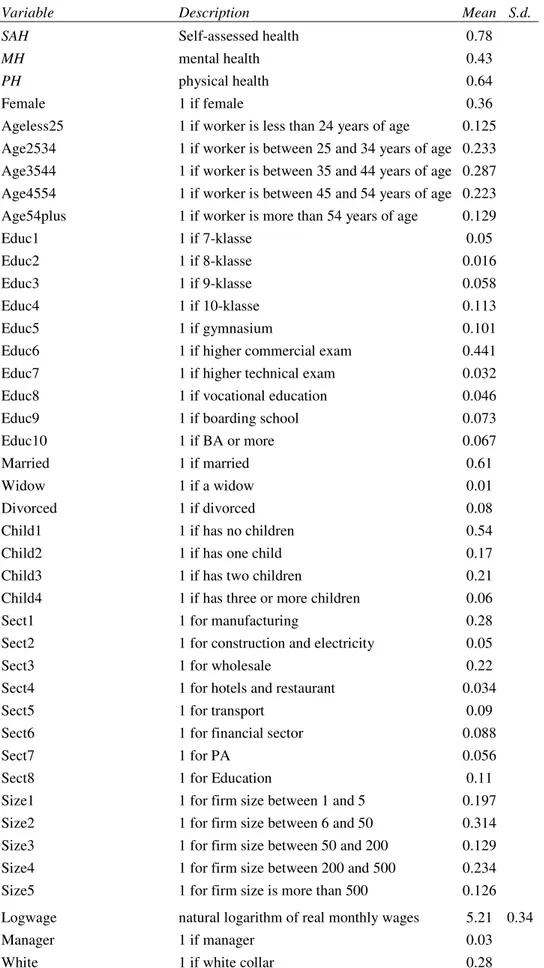
We use a relatively parsimonious set of control variables. As to individual characteristics, we include dummies for gender, age categories, marital status, the number of children in the household, and educational levels. We also control for job characteristics other than adverse working conditions WC through sets of dummies for firm size, sector and occupation. We further control for the natural logarithm of hourly wage and add a time dummy for 2005. A description of the sample is presented in Table A1 in the Appendix.
In Table 1 we show some descriptive statistics on the distribution of health, lifestyle and job quality measures. We observe that self-assessed health is very good or good for
6
With respect to lifestyles we are able to improve over Borg and Kristensen (2000) adding another dimension, that is heavy drinking. Other lifestyle measures that are common in the literature (Belloc and Breslow, 1972; Kenkel, 1995) are excluded from our analyses due either to the lack of a reasonable proxy (as in the case of good sleep) in the dataset or because the definition of the variables changed over time (exercise and good diet).
7 Although measures of smoking intensity are available in the data, we decided to dichotomize the smoking
behavior, for two reasons. First because it is coherent with our empirical model (multivariate probit analysis). Second, and more important, the questions that record intensity of smoking contain many missing values and trying to harmonize them across the two years of the survey made us lose many observations that are necessary to reach convergence in a model as complicated as the one that we are using. This definitely complicates the creation of a smoking dummy variable based on an (arbitrary) intensity threshold for heavy smoking.
8
The definition of the drinking and obesity variables is different across gender. The variable “Drink” takes the value 1 with more than 2 drinks a day for men, and with more than 1 drink in the case of women. About obesity we follow Contoyannis and Jones (2004) and construct an indicator that takes the value 1 if the BMI is greater than 30 for men and greater than 28.6 for women.
10
almost 80% of the employees in the sample. With reference to specific health dimensions, good physical health (in terms of absence of any symptom related to physical problems) is reported by 60% of the sample while good mental health is reported by 40% of the sample.
Table 1. Lifestyles and working conditions by health status (in percentage points)
SAH MH PH Lifestyles: Drinker 0.79 0.4 0.63 Smoker 0.78 0.43 0.57 Obese 0.67 0.4 0.56 Working conditions: Physical hazards 0.79 0.41 0.57 No support from colleagues 0.79 0.36 0.63 Job worries 0.77 0.34 0.57 Repetitive work 0.55 0.55 0.53 Mean 0.72 0.41 0.57
Some of these associations may appear counterintuitive but could be simple compositional effects driven by the spurious correlation between lifestyle, working conditions and health.
4. Empirical strategy
Leaving implicit the subscript for the i-th individual, a simple empirical specification of health equations which accommodates for binary health indicators is the following:
0) > ( = j j j j j j I WC LS X H α +δ +β +ε (1)
where I(#) is an indicator function for the argument being true, H is a health dummy for one of the j dimensions considered: SAH, PH,MH. Xjare explanatory variables such as gender, education, age group, hourly wage and family characteristics. εjare unobservable
individual attributes affecting health; LS includes three dummy variables for obesity, drinking and smoking. WC includes four dummies for physical hazards, repetitive work, feeling no support from colleagues and job worries. Each effect is specific to j-th health
11
dimension considered. We also allow the set of X’s to vary with j, as so do the unobservables.
In principle, the longitudinal nature of our data allows for a dynamic specification, which, for example, included lagged values of lifestyles and working conditions in the health equations (Contoyannis and Jones, 2004) or added lagged health to capture health persistence (see Datta Gupta and Kristensen, 2008). However, in doing so we would lose one wave out of the two available, which is particularly problematic given that our full sample only accounts for about 6,000 observations and that the estimation of our structural model is empirically demanding. As discussed in the Appendix when presenting the theoretical model, we accommodate for the time dimension by interpreting H as an indicator of current and future health. In this way, we can interpret health as dependent also on past lifestyle decisions and working conditions.
In the absence of selectivity issues, (1) could be consistently estimated, e.g., with simple univariate probits. However, the relationship between health vis-a-vis lifestyles and working conditions may be plagued by endogeneity or reverse causality. With respect to the former, unobservable individual tastes may simultaneously affect lifestyles or working conditions as well as the propensity to report physical and mental health problems or low levels of self-assessed health. Economic theory suggests that factors such as risk aversion or the intertemporal discount rate may play a major role.
It is difficult to predict the direction of the endogeneity bias because these two factors may work in opposite directions and differently for different lifestyle choices or working conditions. Consider, for example, smoking and physical health. A higher intertemporal discount rate may increase both the probability of smoking and the importance of past health problems for current health which, in turn, reduces the likelihood of good PH (which is a lack of associated symptoms in the last twelve months). In this case the correlation would be negative. Conversely, a risk-averse individual may be less likely to undertake risky activities such as smoking, drinking or being subject to physical hazards and, at the same time, more likely to report low levels of health. Then, the correlation would be positive.
However, for other key regressors, the correlation may be reversed, for example, if more risk-averse individuals are more worried about their job or have preferences for
12 repetitive jobs.9
Reverse causality arises when, on average, perceived good health influences the propensity of unhealthy behaviour or the probability of being subject to risky working conditions. Again, this may go in either direction and, depending on the variable considered, healthier individuals may trade off their health stock with unhealthy behaviour such as smoking, drinking or weight excess, resulting in a positive error correlation. On the contrary, they may start drinking to substitute the pain of poor mental health. Or they may feel less likely to experience adverse working conditions such as being fired or not being considered by colleagues. In essence, evaluating error correlation patterns is a matter of empirical investigation.
In the Appendix, we sketch a behavioural model that extends Contoyannis and Jones (2004) to include working conditions, and, starting from a static utility maximisation problem in which LS and WC are choice variables, offers insights about the identification of LS and WC genuine effects. The structural model contains both health equations in (1), and health-specific reduced forms for the three lifestyle choices (label k) and the four working conditions (label h): , 0) > ( = k k k I Z u LS γ +
k = smoker, drinker, obese
(2) , 0) > ( = h h h I Z v WC θ +
h = physical hazards, no support from colleagues, job worries, repetitive work
(3)
For each j-th health indicator, (1), (2) and (3) define a fully recursive model that contains eight simultaneous equations freely correlated through unobservables.
The Z vector includes the exogenous covariates in X plus exclusion restrictions. Details about the criteria followed in excluding variables from X and including them in Z are in the next sub-section where we discuss the identification strategy.
We assume normality of the errors and estimate the model by Maximum Simulated
9
Endogeneity may also be effective on the employers’ side, if ‘good’ firms with a pleasant environment are workers’ high-health firm (with health levels higher than expected given observable characteristics) and, at the same time, are less risky in terms of physical and psychosocial working conditions.
13
Likelihood (MSL) as a multivariate probit (MVP) (Cappellari and Jenkins, 2003).10 The structural equations for health (either SAH, MH or PH) and the seven reduced forms for LS and WC are jointly distributed as an eight-variate normal.11 The correlated errors have a correlation matrix estimated together with the coefficients.12 The univariate probits are nested within the MVP framework, when for each j-th health equation,corr(εj,uk)and
) , ( j vh
corrε are zero for all k and h. A simple likelihood test for any of these correlations being zero is informative about the endogeneity of the corresponding variable in the health equation considered.
With our econometric model we can investigate a number of alternative hypotheses about the effect of the k-th lifestyle or the h-th working condition on any j-th health dimension. We can distinguish between four different cases: (1) the correlation coefficient between the errors of the equation k (or h) and j is not statistically different from zero, and the corresponding coefficient in the j-th equation is statistically significant. In this case the variable is exogenous with respect to health and its effect is causal; (2) the correlation coefficient is statistically significant while the coefficient is not. In this case the variable is endogenous and the correlation between errors is driven by unobserved heterogeneity (the so-called third variable hypothesis); (3) both the correlation coefficient and the coefficient
10 Fixed effect estimators for panel data may be used. However, in our case very few individuals change
health status, lifestyles and working conditions over time. This makes both identification and estimation problematic, and we verified that fixed effect estimates are very imprecise and not informative. Accordingly, we treat our sample as a pooled cross section; however, clustering the standard errors at the individual level.
11 In principle one would also allow SAH, MH and PH to be correlated through unobservables, and we
experimented on that. Simple trivariate probit estimates with exogenous LS and WC suggest that, as one may expect, especially the cross-correlation between health variables is always positive and statistically significant. In the multivariate setting, allowing for this additional correlation source complicates the estimation and makes it difficult to get convergence to a global maximum. For this reason, we estimate separately the three health equations in our empirical analysis.
12In general, the identification of pooled models with endogenous regressors is based on variables in Z that do
not appear in X. In our specific case there is, however, another option available: according to Wilde (2000), given the high non-linearity of the recursive multivariate probit model, its parameters are identified through the functional form, with no need of exclusion restrictions. In our empirical analysis we experimented with both identification approaches: we tried to estimate the model, first, without exclusion restrictions. By following the strategy suggested by Wilde (2000), we were able to get estimates for SAH and MH, but not for PH since the likelihood did not converge to a global maximum. However, the results for SAH and MH obtained without exclusion restrictions (available upon request) are very similar to the ones presented in the next section. As a robustness check, we also estimate a different specification of the model with exclusion restrictions, in which, based on joint significance tests, we impose a number of asymmetries in the set of variables excluded from the health equations and used to identify, on the one side, lifestyles, and, on the other side, the set of working conditions. Results are again available upon request and are very similar to the ones discussed in the main text.
14
itself are significant. In this case although the k-th (or h-th) variable is endogenous with respect to j, it also has a causal impact. The estimates of the correlation coefficient and of the causal effect are also informative about the relative importance of the two alternative explanations, i.e. third variable hypothesis vs causal effects; (4) the correlation coefficient and the coefficient itself are both insignificant, and in this case the analysis does not support any of the above hypotheses (see Bratti and Miranda, 2010).
The MVP model is formally identified by the functional form and exclusion restrictions are unnecessary (Wilde, 2000). However, it may suffer from ‘tenuous’ identification, which can be improved setting some exclusion restrictions. They must satisfy two requirements. The first is relevance, i.e. they must shift the net benefit of choosing specific values of LS and WC. The theoretical model sketched in the Appendix suggests that candidate variables are those that exogenously affect income, market and implicit prices of lifestyles and working conditions, the amount of labour time needed to consume one unit of LS and the amount of leisure time needed to consume LS in terms of forgone income.
The second requirement is excludability, i.e. the identifying variables are excludable from the health equations once we control for LS and WC. The guidance offered by the economic theory is subject to the limitations imposed by available information and the lack of sources of truly exogenous variation in the data.13On the one hand, all the covariates included in the analysis - education, age, gender, family status, region of residence; and job characteristics such as the occupation, the size of the firm and the employment sector – are potential shifters of either the direct, indirect and opportunity costs of lifestyle and working conditions. On the other hand, it is difficult to ex-ante justify the exclusion of a subset of these variables (or other variables in the survey) from the health equations.
Given these limitations, the final set of covariates included in each health structural equation are selected using a general-to-specific strategy. We started from a general specification with lifestyles and working conditions plus all the other explanatory variables.
13 Balia and Jones (2008) use family background variables as exclusion restrictions to identify lifestyle
indicators. We also experimented with the approach followed by Contoyannis and Jones (2004), who use one period lags of the exogenous variablesXj as exclusion restrictions for current lifestyle indicators. However, using this strategy only a single cross section is available for the estimates. Maybe because the resulting sample is small as compared to the number of parameters, we encountered several problems to achieve convergence to a global maximum in the likelihood maximization.
15
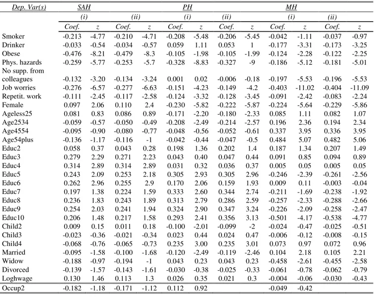
We estimated this general specification by univariate probits, one for each health variable. The results are in columns (i) of Table A2. Then, we run Wald tests for the exclusion of various groups of variables in each health equation. Groups that were statistically significant at 10% level or more were retained in the final specification of the corresponding health equation.14 Through this variable selection process, different covariates were excluded from the final specification of the three health equations and included in Z vectors.
For SAH, exclusion restrictions are sector, size and regional dummies. For PH, we also exclude occupations. For MH, we exclude occupation, size and regional dummies, but we retain sector dummies, which cannot be excluded according to insignificance tests. Hence, joint insignificance tests leave us with asymmetric exclusion restrictions across health measures. On economic grounds, we find it reasonable that different health dimensions have different ‘production inputs’.
In the reduced forms for lifestyles and working conditions, the set of regressors is the same (Z) and includes all the exogenous covariates. Hence, while Z is always the same, we let identification to be health-specific.
Once in columns (ii) of Table A2 we re-estimated the health probits without the exclusion restrictions, the coefficients of retained variables were largely unaffected (compare columns (i) and (ii) results). The stability of the probit estimates with and without the variables used for identification is supportive of our empirical strategy.15
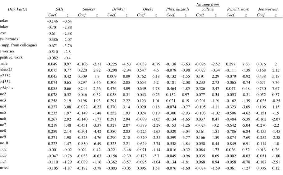
According to Tables A3, A4 and A5, columns (ii) to (viii), exclusion restrictions are also relevant in the first stages: overall, the region of residence, the occupation, the size and the employment sector are statistically significant determinants of lifestyles (being a smoker, a heavy drinker or obese) and of adverse working conditions (being subject to physical hazards, receiving no support from colleagues, doing repetitive stuff, being
14 To ease the presentation, these exclusion Wald tests for the whole battery of controls are not presented here
but available from the authors. However, in the last row of Table 2 we report the test of joint insignificance of all the variables that we exclude from the final specification of each health equation. This test somehow provides an overall assessment about the joint excludability of variables used as a source of identification.
15Of course, an empirically driven identification strategy is a rather informal way to assess excludability
conditions which, in principle, cannot be tested. On economic grounds, these exclusion restrictions suggest that, once we control for WC, LS and other covariates, the health effect of, say, working in firms of given sectors, is absorbed by the fact that, e.g. working in a certain sector means being subject on average to a certain combination of physical and psychosocial working conditions, which is what really matters for individuals’ perceived health.
16 worried about the job).
Back to our economic framework, the regional dummies might capture variability in both exogenous income and the implicit and explicit prices of LS and WC: for example, the average price of alcoholic drinks or cigarettes or the cost of job loss. Interestingly, job-related variables such as occupation, size and sector are able to account for variability not only in working conditions but also in lifestyles. According to our theoretical framework, this is the case when they capture variability in the amount of labour time needed to consume units of LS. For example, companies in different sectors may promote different smoking or drinking policies; similarly, being overweight is more or less compatible with working in certain occupations or in some sectors.16
5. Results
5.1. Self-Assessed Health
Table 2 includes results of the SAH univariate probit with exogenous lifestyles and working conditions and the full recursive multivariate probit. We present Average Partial Effects (APE) for the variables of interest and associated standard deviations plus the statistical significance of the corresponding coefficients.17 Next, Table 3 illustrates error correlations of the fully recursive multivariate model, which are useful in gauging whether lifestyles and working conditions co-vary through unobservables.
As expected, the self-assessed health coefficients of bad lifestyles and adverse working conditions are always negative. This is true for both the exogenous and endogenous models, but with some differences. Simple probit estimates indicate a negative
16 As a consistency check, we also performed a RESET test, which suggests that the health equations are not
misspecified either with or without these restrictions. The RESET test is a useful and generally accepted diagnostic tool in this context, but we must advise that, according to Wooldridge (2002), it cannot be used to test for the presence of omitted variables but only for the miss-specification of the functional form. In a preliminary step, we also estimated the model under alternative identifying assumptions (e.g. by excluding also log of wage and the number of children, which are only weakly significant in columns (i) of Table A2). We find that results are not very sensitive to the choice of variables that may be reasonably excluded from the health equation based on significance tests. This suggests that, as has been found in other papers on similar topics, identification issues may not play a crucial role in the analysis of health determinants.
17The model is estimated by MSL using the command mvprob in Stata. The coefficients of the health equation
estimated by the multivariate probit then are used to compute predicted health probabilities from the univariate standard normal. To get the marginal (i.e. partial) effects we averaged predicted probabilities over individual characteristics. The level of significance of the partial effects in Tables 2, 4 and 6 is that of the corresponding estimated coefficients. They are reported in Table A2, columns (ii) for the univariate probit; and in Tables A3, A4 and A5 in the appendix for the multivariate probit models.
17
and significant effect of smoking and obesity, higher for the latter (13% versus 5% reduction in the probability of reporting good health), while the negative effect of drinking is not statistically significant. All the working conditions negatively affect the probability of reporting good health. The higher importance is attached to job worries and physical hazards, with an APE of about 6%.
Using the 1990 and 1995 waves of Danish data also used by us, Borg and Kristensen (2000) detect a positive statistical association between a worsening in SAH between 1990 and 1995 and smoking and obesity.
Furthermore, adverse working conditions appear positively correlated with a decrease in perceived health. Using a random effect ordered probit, Datta Gupta and Kristensen (2008) similarly find a positive effect of satisfaction for the work environment on SAH.
Once unobservable heterogeneity is accounted for, the overall picture does not change but the negative effects of those variables that maintain statistical significance are even larger. In particular, heavy drinking reduces self-assessed health by about 20% and being obese by about 17%. As a result, unhealthy behaviours imply non-negligible costs on perceived overall health. Conversely, smoking is no longer statistically significant. The error pattern of Table 3 adds useful insights. The correlation between heavy drinking and SAH is positive (0.36), consistent with either a risk aversion interpretation, which may act as a ‘third variable’, or reverse causality, where individuals trade off good health with unhealthy behaviour.
Table 2. Self-assessed health (SAH) estimates (average partial effects, APE)
Probit Multivariate probit
APE St.Dv. Stat. Sign.
coeff APE St.Dv. Stat. Sign. coeff Lifestyles: Smoker -0.049 0.017 *** -0.035 0.016 Drinker -0.008 0.003 -0.196 0.063 ** Obese -0.127 0.035 *** -0.167 0.057 ** Working conditions: Physical hazards -0.057 0.019 *** -0.088 0.040 **
No support from colleagues -0.031 0.011 *** -0.170 0.060 ***
18
Repetitive work -0.026 0.009 *** -0.0192 0.009
N. obs. 6,071 6,071
Log likelihood -2,521.61 -25,278.69
Notes: The multivariate probit estimates are obtained by Maximum Simulated Likelihood with the mvprobit command in Stata with 75 random draws. Full results in terms of estimated coefficients are in Table A2 for the probit model with exclusion restrictions (specifications (iii)) and in Table A3 for the multivariate probit. The APE (average partial effects) are calculated for each observation using the marginal (i.e. univariate) distribution of the health outcome and then averaging over individuals. In the probit case, this is different from using the post-estimation command in Stata dprobit, which evaluates the marginal effect at the mean of observable characteristics. Sample standard deviations, which measure the variation of the partial effects across individuals, are reported along with the corresponding APE. We also report here the statistical significance of the associated coefficient, as taken from Tables A2 and A3. The exclusion restrictions in the probit are the sector, size and regional dummies. Statistical significance of coefficients: * = 10% level; ** = 5% level; *** = 1% level.
For smoking, the correlation is negative and statistically significant, perhaps induced by the intertemporal discount rate. This is in line with the findings of most of the literature (Bratti and Miranda, 2010).
For what concerns working conditions, simple and multivariate probit estimates are qualitatively similar except for the repetitive work’s dummy. In general, the APE is higher in the multivariate specification. This is consistent with the errors’ structure of Table 3, where the correlation between SAH and working conditions is positive and statistically significant in the case of not receiving support from colleagues and job worries. As a result, simple probit estimates tend to underestimate (in absolute value) true SAH effect. According to the discussion in the previous section, positive selection may be driven by reverse causality so that healthier individuals are more able to manage the lack of support or job insecurity. Instead, physical hazards seem to be exogenous to SAH, while for repetitive work we fall into a case (4) (according to the previous section taxonomy) where both the coefficient and the correlation are insignificant.
Our results for SAH are qualitatively similar to those by Contoyannis and Jones (2004), who find a complex correlation structure between errors of SAH and LS equations, and that obesity and physical activity are the only variables who are significant SAH determinants when endogeneity is accounted for. Across groups, there are some interesting differences between physical and psychosocial working conditions: for example, the former are correlated with all of our lifestyle indicators and the latter especially with smoking.
19
conditions is also revealed by Table 3, which shows that there exists a substantial correlation between the reduced forms errors: this is true especially within both physical and psychosocial working condition variables. We also find that physical and psychosocial spheres are correlated to each other.
Longstanding psychological and epidemiological literature has advanced several explanations for why working conditions and behavioural risk factors might be empirically associated with health through unobservables. In general, the idea is that individuals may respond to environmental challenges by modifying their behaviour (Bhui, 2002).18 As smoking is assumed to ease stress, smokers may smoke most when exposed to strenuous work in order to calm themselves down (Perkins and Grobe, 1992; Parrott, 1999).
5.2. Physical and Mental Health
We now investigate whether the effect of LS and WC is heterogeneous across health dimensions. Tables 4 and 6 are the analogues of Table 2 but for a PH and MH models. Tables 5 and 7 report the corresponding matrix of estimated correlation across errors.
We start from PH and look at the effect of lifestyles first. As expected, the probit APE for smoking is negative (-7.5%) and statistically significant and so is for obesity, with an APE of about 4%. However, in the MVP all these effects are statistically insignificant. The inspection of Table 5 reveals that correlation coefficients have the same sign as in the SAH model (all positive except for smoking) but are no longer significant. This is the case (4) of our previous taxonomy, and our analysis is not able to provide any useful prediction about the structural effect of lifestyles on musculoskeletal health.
Probit estimates also suggest that working conditions always play a negative and statistically significant role, with the exception of the dummy for not perceiving support from colleagues. As we might expect, being subject to physical hazard is negatively associated with PH (the APE is 11.7%). Job instability is associated with 5% reduction in physical health, and the APE for repetitive tasks is similar.
18Accordingly, employees might show a tendency to compensate strenuous work, such as heavy physical or
psychosocial demands, with unhealthy behavior. For example, these studies suggest that physically and psychosocially strenuous working conditions and other work-related factors extend their effects outside the workplace and influence the behavior potentially via coping strategies related to drinking or smoking (Greenberg and Grunberg, 1995).
20
Table 3. Correlation coefficients from the multivariate probit for self-assessed health (SAH)
SAH Smoker Drinker Obese Phys. hazards
No support from
colleagues Job worries
Repetitive. work SAH 1 Smoker -0.10* 1 Drinker 0.357** -0.224*** 1 Obese 0.102 -0.093*** -0.026 1 Physical hazards 0.127 0.041* 0.073** 0.118*** 1
No sup. from colleag 0.344*** -0.062** -0.011 -0.021 0.051*** 1
Job worries 0.181* 0.025 0.038 0.014 0.137*** 0.079*** 1
Repetitive work 0.009 0.070** 0.006 0.009 0.188*** 0.021 0.083*** 1 LR-test: All correl. coeffs.
set to zero (no endogeneity) Chi2(28) =282.45; p-value = 0.0000
21
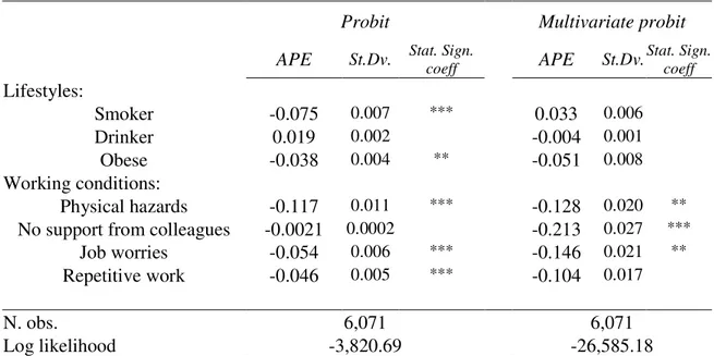
Table 4. Physical health (PH) estimates (average partial effects, APE)
Probit Multivariate probit
APE St.Dv. Stat. Sign.
coeff APE St.Dv. Stat. Sign. coeff Lifestyles: Smoker -0.075 0.007 *** 0.033 0.006 Drinker 0.019 0.002 -0.004 0.001 Obese -0.038 0.004 ** -0.051 0.008 Working conditions: Physical hazards -0.117 0.011 *** -0.128 0.020 **
No support from colleagues -0.0021 0.0002 -0.213 0.027 ***
Job worries -0.054 0.006 *** -0.146 0.021 **
Repetitive work -0.046 0.005 *** -0.104 0.017
N. obs. 6,071 6,071
Log likelihood -3,820.69 -26,585.18
Notes: The multivariate probit estimates are obtained by Maximum Simulated Likelihood with the mvprobit command in Stata with 75 random draws. Full results in terms of estimated coefficients are reported in Table A2 for the probit model with exclusion restrictions (specifications (iii)) and in Table A4 for the multivariate probit. The APE (average partial effects) are calculated for each observation using the marginal (i.e. univariate) distribution of the health outcome and then averaging over individuals. In the probit case, this is different from using the post-estimation command in Stata dprobit, which evaluates the marginal effect at the mean of observable characteristics. Sample standard deviations, which measure the variation of the partial effects across individuals, are reported along with the corresponding APE. We also report here the statistical significance of the associated coefficient, as taken from Tables A2 and A4. The exclusion restrictions in the probit are occupation, sector, size and regional dummies. Statistical significance of coefficients: * = 10% level; ** = 5% level; *** = 1% level.
Similar to what we observed for SAH, MVP effects are larger, except for physical hazards. For example, not being supported by colleagues and job worries reduce PH by 21 and 15%, respectively. Table 5 shows a positive and statistically significant correlation (positive selection) between PH and WC. On the policy side, we show that adverse psychosocial ‘soft’ working conditions are significantly affecting the ‘hard’ dimensions of health, which is not obvious a priori.
Tables 6 and 7 present the results for the MH model. Looking at lifestyle choices, being obese and being a heavy drinker play a major role in simple probits. However, as found in several studies, the latter’s effect is not structural, since it disappears with MVP. The fact that in Table 7 the associated correlation coefficient is insignificant does not allow us to draw any conclusion about the relationship between drinking and mental health.
22
for obesity positive, and both are statistically significant. MVP estimates reveal that being obese increases the probability of suffering from mental health problems by 15%; smoking increases the likelihood of not suffering from mental illness by 16%. Other papers found that smoking has a positive effect on some components of mental health (e.g. Parrott, 1999; Warburton, 1992) suggesting that smoking aids mood control and acts through reducing smokers feelings of anxiety and anger. Of course, a well-known result in the medicine literature is that smoking has severe negative consequences for many health dimensions, which in a policy perspective more than compensate for the positive effect we detect for our mental health measure.
Moving to WC variables, except for repetitive work that is never precisely estimated, they all have a substantial, negative and statistically significant MVP effect on MH. For psychosocial hazards – job worries (APE -12 percent) and not receiving support from colleagues (-19.5 percent) – this is not surprising. The interesting result is that also being subject to physical hazard creates a clear thread to mental health (APE is -21 percent). The inspection of the correlation matrix in Table 7 also reveals a positive association between the physical health and MH unobservables (maybe induced to a ‘third variable’ such as risk aversion), which creates a downward bias in simple probit estimates.
23
Table 5. Correlation coefficients from the multivariate probit for physical health (PH)
PH Smoker Drinker Obese Phys. hazards
No support from
colleagues Job worries
Repetitive. work PH 1 Smoker -0.180 1 Drinker 0.012 0.225*** 1 Obese 0.047 -0.094*** -0.020 1 Physical hazards 0.079 0.041* 0.074*** 0.117*** 1
No support from colleagues 0.386*** -0.064** -0.017 0.018 0.051** 1
Job worries 0.194* 0.024 0.037 0.018 0.137*** 0.083*** 1
Repetitive work 0.127 0.067** 0.004 0.007 0.189*** 0.024 0.084*** 1 LR-test: All correl. coeffs.
set to zero (no endogeneity) Chi2(28) =281.95; p-value = 0.0000
24
Table 6. Mental health (MH) estimates (average partial effects, APE)
Probit Multivariate probit
APE St.Dv. Stat. Sign.
coeff APE St.Dv. Stat. Sign. coeff Lifestyles: Smoker -0.014 0.002 0.162 0.028 ** Drinker -0.060 0.008 *** -0.051 0.011 Obese -0.043 0.005 ** -0.154 0.036 * Working conditions: Physical hazards -0.063 0.007 *** -0.210 0.036 ***
No support from colleagues -0.071 0.008 *** -0.195 0.035 ***
Job worries -0.147 0.017 *** -0.118 0.024 *
Repetitive work -0.029 0.003 ** 0.092 0.019
N. obs. 6,071 6,071
Log likelihood -3,837.90 -26,593.266
Notes: The multivariate probit estimates are obtained by Maximum Simulated Likelihood with the mvprobit command in Stata with 75 random draws. Full results in terms of estimated coefficients are reported in Table A2 for the probit model with exclusion restrictions (specifications (iii)) and in Table A5 for the multivariate probit. The APE (average partial effects) are calculated for each observation using the marginal (i.e. univariate) distribution of the health outcome and then averaging over individuals. In the probit case, this is different from using the post-estimation command in Stata dprobit, which evaluates the marginal effect at the mean of observable characteristics. Sample standard deviations, which measure the variation of the partial effects across individuals, are reported along with the corresponding APE. We also report here the statistical significance of the associated coefficient, as taken from Tables A2 and A5. The exclusion restrictions in the probit are occupation, size and regional dummies. Statistical significance of coefficients: * = 10% level; ** = 5% level; *** = 1% level.
25
Table 7. Correlation coefficients from the multivariate probit for mental health (MH)
s MH Smoker Drinker Obese Phys. hazards
No support from
colleagues Job worries
Repetitive. work MH 1 Smoker -0.327*** 1 Drinker -0.037 0.224*** 1 Obese 0.234* -0.097*** -0.023 1 Physical hazards 0.262** 0.039* 0.074** 0.121*** 1
No support from colleagues 0.264** -0.064** -0.016 0.022 0.053** 1
Job worries 0.118 0.024 0.037 0.015 0.137*** 0.080*** 1
Repetitive work -0.193* 0.068*** 0.005 0.003 0.187*** 0.021 0.085*** 1 LR-test: All correl. coeffs.
set to zero (no endogeneity) Chi2(28) =283.86; p-value = 0.0000
26 6. Conclusions
In this paper we investigate whether employees’ health is affected by adverse working conditions (physical hazards, repetitive work, job worries and not being supported by colleagues) and by risky lifestyles (smoking, drinking and being obese).
We use Danish data for 2000 and 2005, which provide detailed information on lifestyles, working conditions and health matched with individual and establishment administrative records. Our data allow us to define three outcomes: self-assessed health, mental and physical health (not experiencing musculoskeletal problems). Our main set of result is obtained by a multivariate probit approach that accounts for the potential endogeneity of lifestyles and working conditions. We find that in general standard probits tend to underestimate (in absolute values) true effects.
With respect to lifestyles, their effect is negative and statistically significant, especially for self-assessed health. For physical health we are not able to detect any causal relationship. We also find that smoking reduces the likelihood of reporting poor mental health, while obesity works in the opposite direction. Taken at its face value, the first result challenges the common wisdom that good lifestyles practices are important to promoting higher levels of mental well-being, although our mental health indicator refers to specific symptoms (e.g. stress) mediated by individual perceptions.
Physically adverse working conditions matter for both mental and physical health, and their effects on mental health is as much important as that on musculoskeletal diseases. Similarly, psychosocial working conditions - especially in terms of support received from colleagues and worries about job loss - are indeed important determinants of both mental and physical health. This should be taken into account when considering their consequences on workers' well-being.
On the policy side, our results are informative for the design of interventions that promote specific health domains by reducing people’s engagement in health-damaging behaviour and by improving their working conditions.
In a country like Denmark, which is traditionally a pacesetter for safety in the workplace, this may also challenge the perceived effectiveness of policies that in the middle of the last decade promoted good practices to reduce job hazards and improve health levels.
27 Appendix
Theoretical framework
A simple economic model may be useful to summarise the main implications for the empirical analysis of Sections 4 and 5. Our approach is similar to Contoyannis and Jones (2004), whose theoretical model for lifestyle and health choices can be modified to address our case, where health is also a function of working conditions. For simplicity, we consider health as a consumption good which directly affects current utility. The set up can be easily extended to the infinite horizon case, where health is also an investment good as in Grossman (1972), see Balia and Jones (2008). The implications for the empirical analysis are similar.
The individual's utility may be expressed as follows: ) , ; , , (WC LS H XU u U
ε
U is overall utility or satisfaction, which comprises non-work utility (leisure, family time) and work-related utility. The latter depends on a number of job attributes and working conditions WC, which may enter directly the utility function as they are typically not adequately compensated (e.g.: bad working conditions are not fully compensated by higher wages as in Rosen, 1974). At least to some extent, jobs are chosen by individuals, and, therefore, so are their characteristics. Utility is also a function of a bundle of costly activities under the label "lifestyle" LS and of health H. XU
and
ε
u are vectors of individual observable and unobservable (respectively) characteristics affecting preferences.We also assume that health (H) is produced with the following technology:
)
,
;
,
(
=
H
LS
WC
X
H HH
ε
(A1)where XU and
ε
u are exogenous observable and unobservable individual characteristics affecting health. H can be thought of either as a scalar (such as the overall general health of the individual) or as a vector of different and health components: for example, physical and mental health; health at work and health at home and so on. The health production function can be substituted into the utility function to get:) , ; , , (WC LS H X
ε
Uwhere X is the union of the partly overlapping vectors XU and
X
H and similarly for ε.To get the solution to the utility maximisation problem relative to LS, WC and H, we need to combine the above equations with money and time constraints, which, in its compact formulation, can be expressed as follows:
28 wT m TI WC p LS w pLS + LS + LS)' +( WC+ WC)' ≤ = + (
τ
π
π
where m is exogenous income, wT is total labour income if the individual uses all the time endowment T to work at the exogenous wage rate w . pLS and pWC are vectors of market and implicit prices of the goods included among 'lifestyle' choices and 'working conditions'. w
τ
LS isproduct between the opportunity cost of lifestyle practices during leisure time (in terms of forgone income) and the amount of leisure time needed to consume one unit of LS .
π
LS andπ
WC are the amount of labour time needed to consume one unit of LS and WC , respectively. Here the assumption that lifestyles are consumed both at work and at home, while working conditions can be consumed only at work, is implicit. The opportunity cost of lifestyles in non-working time (such as smoking when watching the TV) is forgone labour income, while there is no direct money equivalent for the same activity performed during working time. Hence, (pLS +wτ
LS +π
LS)'LS andWC pWC WC)'
( +
π
are linear combinations expressing the total money equivalent of the overall cost of lifestyles activities and job characteristics.By combining the above expressions for utility and time plus money constraint, the solution of the model is rather straightforward. In this way, the shadow price of each good and, therefore, the demand for each lifestyle and working condition, is dependent on the wage rate, which varies across individuals. In particular, the solution to the model allows us to define a set of demand functions for optimal levels of LS, WC and H:19
) , ( =LS Z
ε
LS∗ (A2) ) , ( =WC Zε
WC∗ (A3) ) , ( =H Zε
H∗ (A4)where Z combines X (the set of exogenous individual characteristics of the model XU and
X
H) and all the parameters used in the maximisation problem (in particular, the wage rate w , prices and time shares). ε is the union ofε
u andε
H. These demand functions are reduced forms and do not allow us to separately evaluate preference and technological parameters, which is the impact of lifestyles and working conditions on health indicators, which is the core of our analysis. The empirical models combine (A1), (A2) and (A3), where the former is the structural equation for health and the other two are reduced forms for lifestyle and health. Finally, a couple of further considerations. First, in the above discussion, we do not consider the effect of the time dimension on actual choices. However, for example in the production of health, the time dimension is indeed19
29
important but can be easily accommodated in a simple way by interpreting H as an indicator of current and future health. In this way, we can think of health as dependent also on past lifestyle decisions and working conditions (compare with Balia and Jones, 2008, who specify a dynamic model for the evolution of health). In principle, this may affect the specification of the empirical model (contemporaneous versus lagged effects). We discussed more on that when describing our estimation methodology (in Section 4). Second, the mapping between the theoretical and the empirical model is of course not perfect. On the one hand, while we have focused on interior solutions, the data reveals the prevalence of corner solutions for lifestyles and working conditions. On the other hand, while we have assumed continuous variables for H, LS and WC – so that utility can be maximised by differentiation to get continuous demand functions – the data often provide instead binary or discrete indicators, such as ordered measures of self-assessed health or dummies for the presence/absence of a given characteristic (e.g. drinking or not).