Design, construction and tests of a high resolution, high dynamic range time to digital converter

(1)

Università degli studi Roma Tre

Scuola Dottorale in Scienze Matematiche e Fisiche

Sezione di Fisica - XXII ciclo

Design, construction and tests of a

high resolution, high dynamic range

Time to Digital Converter

Coordinatore: Relatori:

prof. Guido Altarelli prof. Filippo Ceradini

dott. Paolo Branchini

Salvatore Loffredo

(2)

(3)

Pensiero del giorno per Salvatore: “la vera grandezza è basata non sulla potenza e l’orgoglio culturale, ma sulla vera sapienza la quale fa discernere i veri valori e si trasforma in sorgente di vita... Per essere sapienti occorre anche studiare un po’. Coraggio!” Babbo.

Quanto poi alla misura del tempo, si teneva una gran secchia piena d'acqua, attaccata in alto, la quale per un sottil cannellino, saldatogli nel fondo, versava un sottil filo d'acqua,

che s'andava ricevendo con un piccol bicchiero per tutto 'l tempo che la palla scendeva nel canale e nelle sue parti: le particelle poi dell'acqua, in tal guisa raccolte, s'andavano di volta in volta con esattissima bilancia pesando, dandoci le differenze e proporzioni de i pesi loro le differenze e proporzioni de i tempi; e questo con tal giustezza, che, come ho detto, tali operazioni, molte e molte volte replicate, già mai non differivano d'un notabil momento.

Estratto da “Discorsi e dimostrazioni matematiche intorno a due nuove scienze” di

(4)

(5)

Introduction

The needs of future High Energy Physics (HEP) experiments require the use of time

measurements systems with remarkable benefits in terms of resolution, dynamic range and high operating frequency.

This thesis is focused on the development and evaluation of high resolution and long range Time to Digital Converter (TDC) architectures suitable for the measurement of ~100 nstime intervals,~100 ps resolution and MHz repetition rate in the context of the detectors of the KLOE experiment. The KLOE experiment has been designed in order to record e+e- collisions at DAΦNE, the ϕ-factory at the Laboratori Nazionali di Frascati.

DAΦNE collider operates at high luminosity at the center of mass energy corresponding to the mass of the ϕ resonance, 1020 MeV. The ϕ-meson decays mostly to kaon pairs. The ϕ production cross section peaks at about 3 μbarns. Many interesting physics measurements can be performed with the

luminosity reached by DAΦNE (5×1032

cm-2 s-1); more than thousand ϕ-mesons are produced per second. The rate of e+e-  e+e- elastic scattering and e+e-  e+e- X via  interaction is much higher. The trigger and data acquisition systems of the KLOE experiment allow for a repetition rate of about 20 kHz.

The thesis work is aimed to the specific requirements of the HEP experimental environment; nevertheless, it is also useful in many applications of science and industry where high resolution time measurements are required.

The structure of this thesis is organized as follows.

In the first chapter, the DAΦNE collider and the KLOE experiment are described. A brief description of the physics goals of the experiment and the systems needed to achieve it are given. In the second chapter a review of methods for time interval measurements is given; the basic and most important parameters of a TDC are described.

(10)

The third chapter is dedicated to the two TDC architectures implemented in a Field Programmable Gate Array (FPGA) device.

The fourth chapter describes the TDC tester board, that I built in order to test the TDC architectures, and the test environment.

In the fifth chapter, I compare the two architectures and show their performance in terms of stability and resolution.

(11)

Chapter 1 Physics with KLOE

1.1 Introduction

The scientific program with a high-performance detector such as KLOE (K-Long Experiment) covers several fields in particle physics: from measurements of interest for the development of the Effective Field Theory (EFT) in quark-confinement regime to fundamental tests of Quantum Mechanics (QM) and of discrete symmetries, CP and CPT invariance. It includes precision measurements to probe lepton universality, the Cabibbo-Kobayshi-Maskawa (CKM) unitarity and settle the hadronic vacuum polarization contribution to the anomalous magnetic moment of the muon and to the fine-structure constant at the MZ scale.

During year 2008 the Accelerator Division of the Frascati Laboratory has tested a new interaction scheme on the DAΦNE (Double Annular ϕ-factory for Nice Experiment) ϕ-factory collider, with the goal of reaching a peak luminosity of 5×1032 cm-2 s-1, a factor of three larger then what previously obtained. The test has been successful and presently DAΦNE is delivering up to 15 pb-1/day, with solid hopes to reach soon 20 pb-1/day [1,2]. Following these achievements, the data-taking campaign of the KLOE detector on the improved machine that was proposed in 2006 [3], will start in 2010.

1.2 DAΦNE

The DAΦNE layout is shown in figure 1.1. The collider is made of two storage “rings” in which

120 bunches of electrons and positrons are stored. Each bunch collides with its counterpart once per turn. The two separate rings scheme is intended to minimize the perturbation of each beam on the other. Electrons and positrons are injected in the rings in bunches separated by 2.715 ns at the energy of ~510 MeV, and collide at an angle of (π – 0.025) radians. Electrons are accelerated to the final energy in the Linac (Linear Accelerator), accumulated and cooled in the accumulator ring and injected in the electron ring with a transfer line.

(12)

Figure 1.1: The DAΦNE complex.

Positrons require first electrons accelerated to 250 MeV to an intermediate station in the Linac, where positrons are created in a thin target, then follow the same processing as electrons and are injected with another transfer line. Since the stored beam intensities decay rapidly in time, the cycle is repeated three-four times per hour. The luminosity is defined by the beam parameters:

(1.1)

where n is the number of the bunches, each collecting N particles, ν is the revolution frequency in the storage ring (367 MHz), and are the standard deviations of the horizontal and vertical transverse beam profile at the interaction point.

DAΦNE runs mostly at a center-of-mass energy of Mϕ  1019.45 MeV. The ϕ production cross

section is σ (e+

e- →ϕ)  3.1 μb. The dominant ϕ meson decays [4] are shown in table 1.1.

Table 1.1: Main branching ratios of ϕ meson decays .

4 _x _y N N L n      x  y

(13)

1.3 KLOE

KLOE is a multipurpose detector, mainly consisting of a large cylindrical Drift Chamber (DC)

with an internal radius of 25 cm and an external radius of 2 m, surrounded by a sampling fibers calorimeter (EMC) organized in a barrel and two end-caps. Both DC and EMC are immersed in the 0.52 T axial magnetic field of a superconducting solenoid.

The design was driven by the intent of being a definitive high precision experiment, while the size was dictated by the long decay length of the KL meson. Kaons from ϕ mesons decaying at rest

travel at approximately one fifth of the speed of the light; the mean path travelled by a KL meson

L = c is 3.4 m; with a radius of about two meters, KLOE can catch 50% of KL decays.

Peculiar to KLOE is the spherical, 10 cm radius, beam pipe which allows all of the K0s mesons

produced in ϕ meson decays to move in vacuum before decaying (S is 6 mm). Details of the

detector can be found in refs. [5-9]. A transverse view of the KLOE detector is shown in figure 1.2.

Figure 1.2: Cross-sectional view of the KLOE experiment, showing the interaction region, the DC, the EMC, the superconducting coil, and the return yoke of the magnet, the beam pipe with the spherical insertion, the

(14)

From 2000 to 2006, KLOE has acquired 2.5 fb-1 of data at the ϕ(1020) peak, plus additional 250 fb-1 at energies slightly higher or lower. A collection of the main physics results of KLOE can be found in Ref. [10].

1.4 KLOE-2

For the forthcoming DAΦNE run [11], upgrades have also been proposed for the detector; the

entire plan of the run is referred as the KLOE-2 project [12]. In a first phase, two different devices named Low Energy Tagger (LET) and High Energy Tagger (HET) will be installed along the beam line to detect the forward scattered electrons/positrons from  interactions. Two LET detectors will be installed at about 1 meter away from the interaction point (inside KLOE); while two HET detectors will be installed at about 11 meters away from the interaction point, just after the first bending magnets. The positions for these tagging detectors were chosen on the basis of the DANE magnetic elements, used as a beam spectrometer, and the available free space along the beam lines. The two e+e- energy ranges they explore are: 160-230 MeV for the LET and 425-490 MeV for the HET. Figure 1.3 shows the positions of the detectorsalong the beam line.

Figure 1.3: Top view of the DAΦNE storage rings showing a cut-out ofthe KLOE experiment, the HET and the LET positions along the beam line.

The LET detector is composed by a LYSO crystal matrix with SiPM read-out; the front end electronic is outside KLOE. The HET hodoscope is composed by two rows of scintillators with PMT read-out.

(15)

In a second phase, a light-material Internal Tracker (IT) will be installed in the region between the beam pipe and the drift chamber to improve charged vertex reconstruction and to increase the acceptance for low pT tracks [13]. Crystal Calorimeter with Timing (CCALT) will cover the small

polar angle region, aiming at increasing theacceptance for forward electrons/photons down to 8°. A new sampling calorimeter (Quadrupole Calorimeter with Timing, QCALT) made of scintillator tiles will be used to instrument the DAΦNE focusing system for the detection of photons coming from KL decays in the drift chamber. The QCALT is replacing the QCAL (Quadrupole tile

Calorimeter) shown in figure 1.2.

The task of QCALT calorimeter is to identify photons from KL → π0π0π0 decays that would mimic

the CP-violating decayKL → π0 π0 decay if the photon would be absorbed by the DAΦNE focusing

system. Figure 1.4 shows the forthcoming detector upgrades.

Figure 1.4: Forthcoming detector upgrades.

1.5 The KLOE electromagnetic calorimeter

The KLOE electromagnetic calorimeter [6], shown in figure 1.2, is a spaghetti like calorimeter

built with lead and scintillating fibers. The lead foils are 0.5 mm thick and shaped with grooves to accommodate the scintillating fibers.

A single module is built with 200 lead-scintillating fibers layers held together by gluing. The structure is such that the response and the energy resolution are independent from the direction of the particles, thus it behaves like a homogeneous calorimeter.

The barrel modules are 4.30 m long and have a trapezoidal shape with bases 52 and 59 cm long and height 25 cm. An additional 32 modules with rectangular cross section, are wrapped around each pole piece of the magnet yoke to form the end-caps, which hermetically close the calorimeter up to ~ 98% of 4π. The fibers run parallel to the axis of the detector in the barrel, vertically in the end-caps, and are connected at both ends to light guides. The read-out is through photo-multipliers

(16)

located at both sides of the module. The arrival times of the scintillation light are used to determine the position along the module. The calorimeter read-out granularity is defined by the light collection segmentation. The fiber’s direction is referred to in the following as longitudinal. The energy is determined through the measurement of the integrated charge of the photo-multipliers.

The primary functions of the electromagnetic calorimeter are the measurement of photon (electron) cluster energies and position. It also provides an accurate measurement of the time of arrival of particles.

Photons occur copiously in the decay of neutral pions, for example from KSKL → nπ0’s as well as

from many other products of ϕ-decays. The determination of the distance that KL-mesons have

travelled before decaying to π0_{’s is of crucial importance in the study of CP violation. The travelled}

path is obtained from a measurement of the time of arrival of photons from π0

decays. Since neutral kaons from ϕ-mesons decaying at rest travel with a velocity β ~ 1/5, time measurements with a precision of 100 ps allow to determine the flight path of a KL decaying in nπ0 with a precision of

about 0.6 cm, for a single detected photon.

1.5.1 Clustering

The calorimeter segmentation provides the determination of the position of energy deposits in r-ϕ for the barrel and in x-z for the end-cap. A calorimeter segment is called in the following a cell and its two ends are labeled as A and B. For each cell, two time signals, tA,B and two amplitude

signals SA,B are recorded from the corresponding PM’s signals. The times tA,B (in ns) are related to

TA,B, the times in TDC counts, by the equations:

(1.2)

Where cA,B (in ns/TDC counts) are the TDC calibration constants. The longitudinal position of the

energy deposit is obtained from the difference tA – tB.

The particle arrival time t and its coordinate z along the fiber direction, the zero being taken at the fiber center, are obtained from the times tA,B as:

(1.3)

(1.4)

Where t0A,B are the overall time offsets, and L and υ are respectively the cell length (cm) and the

light velocity in the fibers (cm/ns). The energy signal, E, on either side of a cell i is obtained from the signals SA,B as:

, , , A B A B A B t c T 0 0 ( ) 2 2 2 A B A B t t t t L t ns       0 0 ( ) ( ) 2 A B A B z cm  t   t t t

(17)

(1.5)

All signals S above are in ADC counts. S0,i are the zero-offsets of the amplitude scale. Smip,i is the response for a minimum ionizing particle crossing the calorimeter center. Dividing by Smip,i equation 1.5 above accounts for PM response, fiber light yield and electronics gain. kE gives the

energy scale in MeV, and it is obtained from showering particles of known energy.

In order to obtain a calorimeter response independent of the position, a correction factor AiA,B(s),

due to the attenuation along the fiber length, is applied. The cell energy, Ei, is taken as the mean of

the determinations at both ends:

(1.6)

The determination of the absolute energy scale relies instead on the use of the monochromatic source of 510 MeV photons; the e+e- → γγ sample. This calibration is routinely done each 200-400 nb-1 of integrated luminosity (i.e. approximately every 1-2 hours during normal data taking). For the timing, the relative time offsets of each channel, ti0, related to the cable lengths and electronic

delays and the light velocity in the fibers are evaluated every few days with high momentum cosmic rays selected with Drift Chamber information. An iterative procedures uses the extrapolation of the tracks to the calorimeter to minimize the residuals between the expected and measured times in each cell. A precision of few tens of picoseconds is obtained for these offsets.

The clustering procedure associates different hits in the calorimeter cells in a single cluster as due to the same particle. Each group collects hit cells close to each other in space and time. Among these, the cell with highest energy release is found; then, the nearest hit cells are associated to the highest one, in order to reconstruct a cluster.

The cluster energy is obtained by adding the energy released in the nearest cells:

(1.7) where i is the index of the cell number.

The cluster position is evaluated as the energy-weighted average of the cell coordinates:

(1.8)

where , zi is the cell coordinate along the fiber (see equation 1.4), and xi, yi are the

nominal positions of the cell.

Finally, the cluster time is obtained in an analogous way: 0, , , , ( ) , i i i A B A B A B mip i E S S E MeV k S    ( ) 2 i i i i A A B B i E A E A E MeV   clu i i E 



E i i i clu i i E R R E 



( , , ) i i i i R  x y z

(18)

(1.9) where ti are evaluated as in equation 1.3.

1.5.2 Time, energy and spatial resolution

After the description of the calibration and monitoring procedures, the resolution of the calorimeter is here summarized.

Figure 1.5: Top left: Linearity of the energy response (Eclu-Eγ)/Eγ as a function of Eγ; Bottom left: Energy

resolution as a function of Eγ; both curves are obtained with radiative Bhabha events e+e-γ; the fit result

obtained is given by equation 1.10. Right: Time resolution as a function of Eγ for ϕ radiative decays.

The energy resolution function (see figure 1.5 on the left side) is determined with radiative Bhabha events, e+e- → e+e-γ, where Eγ is measured by the e+e-DC tracking:

(1.10)

The intrinsic time resolution is dominated by photoelectron statistics (see

figure 1.5 on the right side).

A constant term determined from e+e- → γγ, radiative ϕ decays and ϕ → π+π-π0 events has to be added in quadrature. This constant term is shared between a channel by channel uncorrelated term and a term common to all channels. The uncorrelated term is mostly due to the calibration of the time response of each cell, while the common term is related to the uncertainty of the event T0,

arising from the DAΦNE bunch-length and from the jitter in the trigger phase-locking to the

i i i clu i i E t T E 



0.057 ( ) E E E GeV  _ 57 / ( ) t ps E GeV  

(19)

machine RF. By measuring the average and the difference of Tclu – Rclu/c for the two photons in ϕ

→ π+_π-_π0

events, a similar contribution of ~100 ps for the two terms has been estimated. Thus the resolution is:

t 57ps/ E GeV( )100ps

( 1.11)

In the same way, using control samples where the photon direction is measured with the DC, the cluster position resolution function has been determined. The resolution is 1.3 cm in the coordinate

transverse to the fibers and of in the coordinate along the fibers. This enables to

localize the γγ vertex in KL → π+π-π0 decays with σ ≈ 2 cm along the KL line of flight, this is

determined by the direction of the associated KS meson.

1.5.3 TDC of the KLOE electromagnetic calorimeter

The main constraint for the KLOE EMC TDC design[14, 15] is to maintain the time resolution of the calorimeter response. For this, it must have excellent performances in terms of resolution, linearity and stability. The dynamic range is defined by the kinematics of kaon decays and it is fixed at 220 ns, a ~1 cm resolution implies a time resolution of 33 ps that can be obtained with a 12-bit time encoding.

Each TDC channel is built around a monolithic Time-to-Analog Converter (TAC) developed in bipolar technology, preceded by a delay circuit, as shown in figure 1.6. The TAC function principle will be described in the following chapter. In this method, the time interval is first converted into a voltage by linearly charging a capacitor with a constant current and then the voltage is held briefly to allow the analog-to-digital conversion. The digitization least significant bit is of 53 ps.

The EMC TDC works in common start mode, the start is provided by the fast first-level trigger signal T1 and the stops are provided by the KLOE EMC discriminators [16] output.

Figure 1.6: KLOE EMC TDC analog input section.

(20)

The trigger signal T1, which start the TAC conversion, is synchronized with the bunch crossing time and arrives 200-300 ns after the collision time at a rate of ~20 KHz [17]. In order to compensate for the delay of T1, the stop signals are delayed by a monostable multivibrator at the input of each channel.

The EMC TDC performances, measured on the 4880 calorimeter read-out channels, show a pedestal RMS spread less than one count, an integral non linearity of less than 0.2% of full scale and a temperature stability better than ± 0.3 count/°C.

1.6 Tile and crystal calorimeters for KLOE-2 experiment

The upgrade of the DAΦNE layout requires a modification of the size and position of the low-

quadrupoles located inside the experiment, thus asking for the realization of two new calorimeters covering the quadrupole area. To improve the reconstruction of KL → 2π0 events with photons

hitting the quadrupoles a calorimeter with high efficiency to low energy photon (20-300 MeV), time resolution of less than 1 ns and a space resolution of few cm, is needed. The QCALT (shown in figure 1.4) matches these requirements; it has a dodecagonal structure, 1 m long, covering the region of the new quadrupoles composed by a sampling of 5 layers of 5 mm thick scintillator plates alternated with 3.5 mm thick tungsten plates, for a total depth of 4.75 cm (5.5 X0).

The active part of each plane is divided into twenty tiles of ~5×5 cm2 area with 1 mm diameter plastic wavelength shifting (WLS) fibers embedded in circular grooves. Each fiber is then optically connected to a silicon photomultiplier of 1 mm2 area, SiPM, for a total of 2400 channels.

The arrangement of the WLS fibers allows the measurement of the longitudinal z coordinate by time difference. Although the tiles are assembled in a way to optimize the efficiency for photons originated in KL decays, a high efficiency is in fact also obtained for photons coming from the IP.

Moreover, the low polar angle regions (below 18°) need the realization of a dense LYSO (Lu18Y2SiO5:Ce) crystal calorimeter with very high time resolution performances to extend the

acceptance for multiphotons events, the CCALT (shown in figure 1.4). The most important characteristics of these crystals are a very high light yield, a time emission, τ, of 40 ns, high density and 1/X0 without being hygroscopic. The project consists in a dodecagonal barrel for each side of

the interaction region, composed by LYSO crystals (2x2x13 cm3) read-out using avalanche photodiodes (APD). This allows to increase the acceptance for forward electrons/photons down to 8°.

(21)

1.7 Time measurements in KLOE-2

The bunch identification can be obtained using a TDC with a resolution better than 0.5 ns since the inter bunch time difference is 2.715 ns. In this thesis I describe a TDC architecture that allows a resolution in the range of 20 ps. With such a resolution we should be able to improve the signal/background ratio by using a constrained fit on the kinematic of the event. The dynamic range of the described TDC is about 8 seconds which is far more than we need in KLOE since the KL

lifetime is about 50 ns.

Moreover such a TDC is based on a flash architecture. This implies a dead time of 12.7 ns. Such a device can therefore be used in high trigger rate environment like Super B Factories where the estimated trigger rate is about 150 kHz at a luminosity of 1036 cm-2 s-1.

(22)

(23)

Chapter 2 Review of methods for time interval measurements

2.1 Introduction

Time interval measurements between two or more physical events are often required in many

applications in High Energy and Nuclear Physics. Such experiments are aimed in mean life-time measurements of excited states, angular correlation functions, time-of-flight measurements and particle identification. Usually the time interval is measured between the leading edges of a START and a STOP signal. These signals may be generated by the front-end electronics used to extract the timing information coming from a particle detector. Particles interacting with the detectors generate electrical signals (charge, current or voltage) which have to be measured with the best accuracy, stability and resolution consistent with the experimental requirements. The detector signals are processed by the front-end electronics that usually is built by amplifiers, shaper circuits and discriminators. The front-end electronics deliver the START and STOP signal to the Time-to-Digital Converter (TDC) that performs the conversion of the time interval into a binary word, which can be displayed in a decimal form. So the accuracies and resolution of a time measurement in physics experiments takes into consideration the contribution from all the components of the system: the detector, the front-end electronics and the TDC. Figure 2.1 shows a simplified view of a TDC with two separate inputs of START and STOP.

(24)

2.2 Conversion basics

The characteristic parameters of a TDC are:

- The range of measurements, which is the largest time interval that can be measured.

- The standard measurement uncertainty, expressing the time interval resolving capability of a TDC, i.e. the standard deviation of the measurements distribution around the mean value, when a constant time interval is measured several times.

- The resolution, which is the least significant bit of the binary word read and then the smallest time interval measured.

- The reading speed or how fast is the tool to produce the measurements result. This parameter is important when measurements are made in continuous way at high frequencies and with real time readings.

- Non-linearity of the time-to-digital conversion: differential and integral, expressing the deviation from the ideal behaviour of the converter.

Figure 2.2 (left) shows the ideal transfer function of a TDC, which displays the conversion of a time interval in a binary word, each corresponding to one step of the curve; this will inevitably include [18] a quantization of the measurement. Figure 2.2 (right) shows the real transfer function from which is noticed the deviation from the ideal case that is usually measured by the differential and integral non-linearity.

Figure 2.2: TDC transfer function. Left: ideal case. Right: real case.

The differential non-linearity (DNL) is:

i i LSB LSB DNL LSB   (2.1) Where LSBi is the i-th time interval corresponding to the Least Significant Bit of the i-th bin. The

(25)

the bin width for a given binary value output and the average width of the bin calculated over the entire measuring range; the difference is then divided by the average value of the bin.

The integral non-linearity is: 1 1 j i j i LSB LSB INL M LSB   



(2.2)

The INL is determined for a bin j from the sum of previous differential non-linearity until the bin j, this sum is divided by the total number M of bin of the TDC. To describe the linearity error by a single value, usually the maximum value of INLj or INLj max (1 j M) is selected, which

represents the worst case.

2.3 Precision frequency standards

Several different types of devices are used to generate high precision clock signals, as uncompensated crystal oscillators (XO), temperature-compensated crystal oscillators (TCXO), oven-controlled crystal oscillators (OCXO) or atomic frequency standards; the progress achieved in terms of performance of these devices leads to the characterization of their frequency stability. The output voltage of a sinusoidal generator can be written in the following form:

u t( )(U₀( ))sin(2t ₀t( ))t (2.3) U0 is the nominal value of the amplitude and 0 the nominal value of the frequency. In the

following, is assumed that the amplitude fluctuation ε(t) is negligible in comparison with U0 and is

considered only the phase fluctuation (t). The Greek letter ν is used to indicate the signal frequency while the Latin symbol f is used as frequency variable in the Fourier representation of the signal. The frequency of the sinusoidal voltage is equal to:

( ) ₀ 1 ₀ 2 v d t dt           (2.4) and is the sum of a constant nominal value 0 and a variable term:

1 2 v d dt     (2.5) The normalized frequency offset from the nominal frequency of the signal is designated by y(t) and defined as follows: 0 0 1 ( ) 2 v d y t dt       (2.6) Another useful quantity is the time integral of y(t):

0 0 ( ) ( ) ( ') ' 2 t t x t y t dt   

_

 (2.7)

(26)

and also:

( )y t dx dt

 (2.8) The normalized frequency offset y(t) and the phase-time x(t) are to be interpreted as random processes and can be described by statistical method.

Most real oscillators not only exhibit random frequency variations about a nominal average but also a systematic frequency drift with time:

y t( ) y t_r( ) at y₀ (2.9) and also: ( ) ( ) 2 ₀ 2 r a x t x t  t y t (2.10) where a is a normalized aging coefficient, y0 an initial offset and yr, xr the truly random processes.

It’s assumed that the mean value of yr over the period of observation is equal to zero, furthermore

it’s always possible to subtract the drift term at and y0 from the data; then is assumed that also y(t)

have a zero mean value over the time of observation.

The result of a frequency measurement is always obtained as an average over a finite time interval τ, any sample is of the form:

( , ) 1 ( ) 1( ( ) ( )) k k t k k k k t y t y t dt x t x t       



   (2.11)

The measurements are taken at regular time intervals T= tk-1-tk, with dead time T-τ. For a series of

N measurements the results are:

y tk( , )k   y₁, y₂,...,yN (2.12)

The mean value is:

1 1 N k N k k y y N    



(2.13) and the variance of the sample of N values:

2 2 1 1 ( , , ) ( ) 1 N y k k N k N T y y N        



(2.14)

According to the assumption made above, the limit should be: lim k N 0

N  y (2.15)

whereas the limit

lim 2_y( , , ) 2( )

(27)

should tend to the variance σ2_{(τ) of the process if such a limit exists. Even after elimination of any}

initial offset and linear drift, it is found that the sample variance σy2(N,T,τ) depends on all of the

three variables N, T and τ. The sample variance defined in (2.14) is therefore not useful to describe experimental data in the time domain. A possible solution to this problem has been proposed by D.W. Allan [19] and J.A. Barnes [20] who have shown that for limited values of N, T and τ the limit: 2 2 1 1 ( , , ) lim ( , , ) M y yi M i N T N T M      _   



(2.17)

exists in many cases of interest where the limit (2.16) does not exist. The average of the sample variance as defined in (2.17) is referred as Allan variance.

The behaviour of y(t) in the frequency domain is described by its spectral density Sy(f) which is

defined in the usual way as the Fourier Transform of the auto-covariance Ry(τ), as follows:

0 1 ( ) lim ( ) ( ) T y T R y t y t dt T       



 (2.18)

Then the spectral density is defined according to the Wiener-Khintchine relation [21] as: 0 ( ) 4 ( ) cos 2 y y S f R    f d  

_

(2.19)

The relation between the spectral density Sy(f) and the general form of the Allan variance is [22,23]:

2 2 0 ( , , ) ( ) | ( ) | 1 y y N N T S f H f df N       



(2.20) where: 2 2 2 2 2 2 sin sin | ( ) | 1 ( ) sin f rf N H f f N rf            _  _   (2.21) and r = T/τ.

The main reason why the Allan variance has become a useful parameter for the characterization of frequency stability is that the integral of (2.20) has the property of existing even for some cases of non-integrable (infinite power) spectral densities.

The Allan variance for N = 2 has another advantage which is the extreme simplicity of computation from measured data:

2(2, , ) 1 ( ₁ )2 2

y T yk yk

  _

      (2.22) In several applications it is possible to make the measurements with negligible dead-time. It then can be assumed that T = τ. The N=2, T=τ Allan variance has been proposed as a recommended measure for frequency stability in the time domain. It is usually designated by:

(28)

2 2

( ) (2, , )

y y

       (2.23) Some authors use the term Allan variance for this special case only.

The types of noise observed on the output signal of an oscillator can be represented most suitably by means of the spectral density Sy(f). In practice, these random fluctuations can often be

represented by the sum of five independent noise processes, and hence:

2 2 for 0 ( ) 0 for h y h h f f f S f f f     _{ }     _ 



_(2.24)

where hα’s are constants, α’s are integers, and fh is the high frequency cut-off of a low pass filter.

High frequency divergence is eliminated by the restrictions on f in this equation. In the special case of N= 2, T = τ the Allan variance is:

4 2 2 2 0 2 sin ( ) (2, , ) y y y u u T S du u              _ _  



(2.25) where u=πfτ.

Then, the relationship between the Allan variance and every term of the form hαfα is:

2 ₁ 2 4 0 2 ( ) sin ( ) h f y h u udu  _        



(2.26) that is: 2 ( ) y K       (2.27) with μ=-α-1 and 2 4 1 0 2 sin fh h K u udu     _



 .

Information about the spectral densities Sy(f) can be obtained from time-domain measurements of

σy(τ) versus τ on double logarithmic scale, this kind of plot yields segments of straight lines in the

ranges of τ where one of the various term hαfα or Kατμ dominates.

The widely used standard frequency sources are [24][25]: - caesium-beam resonators;

- hydrogen masers;

- hydrogen storage beam tube; - methane saturated absorption cells; - rubidium vapour cells.

Furthermore, quartz-crystal oscillators, without being accurate frequency standards, are of high importance as slave oscillators in all radio frequency standard.

The caesium atomic beam is produced from a heated oven containing liquid caesium. The first state selector allows only atoms of a selected hyperfine state to pass through the interaction region, where

(29)

transitions are produced by a pair of separated oscillating fields (Ramsey method) in a microwave cavity (ν0=9.2 GHz). Simultaneously a uniform weak magnetic field (C-field) is applied in order to

separate the different sublevels of the hyperfine state, so the transitions occur only between the two levels (mF=0), where the Zeeman effect is purely quadratic. The second state selector allows only

atoms that have completed the transition to the other hyperfine state to be detected. The caesium atoms are detected by surface ionization on a hot-metal ribbon. Usually the ion current is amplified by means of a secondary electron multiplier. As a function of excitation frequency, the output current shows a sharp resonance peak. Figure 2.3 shows the principle of caesium beam frequency standard.

Figure 2.3: Principle of caesium beam frequency standard.

In the Hydrogen masers, the atomic hydrogen is produced in a radio frequency discharge source and the beam is formed in a collimator. Atoms in the upper hyperfine state are focused into a coated storage bulb by means of a multipole magnet. The storage bulb is located in the uniform radio frequency field region of a high Q cavity. A weak uniform magnetic field is applied for the same reason as in a caesium tube. The condition of oscillation depends on various relaxation process, the flux ratio of atoms in the desired and undesired states, and the loaded Q of the tuned cavity. Figure 2.4 shows the principle of hydrogen maser frequency standard.

(30)

Hydrogen storage beam tubes combine the advantages of the passive resonator with those of hydrogen atom storage in a coated bulb. Source and first state selector are similar to those of a hydrogen maser. An output collimator, a second state selector and hydrogen atom detector are added to the storage bulb. Figure 2.5 shows the principle of hydrogen storage beam frequency standard.

Figure 2.5: Principle of hydrogen storage beam frequency standard.

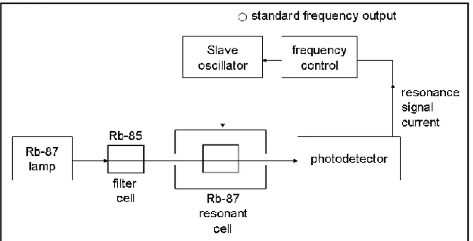
Figure 2.6 shows the principle of rubidium vapour cell frequency standard. A light beam from an

87

Rb lamp, filtered by a vapour cell containing 85Rb, depopulates one of the two hyperfine levels of

87

Rb atoms stored in another cell which is located inside a cavity. Figure 2.7 shows the simplified energy level diagram in which the resonance radiation of the 87Rb lamp is filtered by means of the

85

Rb isotope absorption in such a way that there are more transitions from the 5S1/2 F=1 level up to

the 5P3/2 level than from the 5S1/2 F=2 level. The lower ground state hyperfine level 5S1/2 F=1 is

thus depopulated. Absorption on the 7800 angstrom wavelength then ceases until the application of the 6834 MHz microwave radiation to the cavity.

(31)

The latter repopulates the lower level by means of induced transitions from the F=2 down to the F=1 level and absorption of the 7800 angstrom pumping radiation is again observed at the photodetector, which thus provides the resonance signal for locking the slave oscillator. With high levels of pumping light, appropriate choice of buffer gases, and high Q cavity, maser oscillation can be obtained. In practical applications, however, the passive mode of operation is the only one used. This is the simplest and least expensive type of atomic frequency standard and it has found wide acceptance for those applications where its ageing with time is non inconvenience. An even simpler variety, using natural rubidium in a resonance cell without additional filter cell is also used.

Figure 2.7: Simplified energy level diagram.

Methane saturated absorption cell is a high accuracy frequency standard in the infrared region. A gas cell filled with methane is mounted with a 3He-20Ne gain cell between the two mirrors of a laser cavity. The He-Ne laser can be made to oscillate at a frequency of approximately 88 THz (wavelength 3.39 μm) which coincides with a resonance of the methane molecule. With appropriate methane pressure, strong absorption occurs over the whole range of oscillation of the laser. Methane molecules in the cell interact with both running waves forming the standing wave pattern in the Fabry-Perot resonator of the laser system.

(32)

Molecules having arbitrary velocities are perturbed at two different frequencies because of the first order Doppler shift which is of opposite sign for each running wave. For the molecule moving in a direction perpendicular to the laser beam, the Doppler shift vanishes. These molecules are perturbed by a signal at twice the amplitude without Doppler shift. If the intensity of the laser radiation is sufficiently high and its frequency adjusted, the lower energy level of the molecular transition is depopulated. Additionally, photons will be re-emitted coherently through induced transitions. Therefore, less energy will be absorbed from the laser beam if its frequency is that corresponding to the molecular transition. This phenomenon is called saturation and the dip in the absorption line profile known as the “Lamb dip”. The resonance signal is observed by means of a photodetector. The frequency of the He-Ne laser is modulated for scanning the resonance by means of a piezoelectric transducer moving one of the laser mirrors. The average frequency is locked to the methane resonance by means of an electronic servo system.

Table 2.1 shows the state of the art in the accuracy capability of crystal oscillators and commercial atomic frequency standards [26]. Figure 2.9 shows a time-domain measurements of σy(τ) versus τ of

precision commercial and laboratory frequency standards [26].

Table 2.1: Accuracy capability of crystal oscillator and commercial atomic frequency standard.

(33)

2.4 The Nutt method

The Nutt method [27] combines different time measurements with different ranges and accuracies into one; it’s usually used when a large linear dynamic range and high resolution are needed simultaneously. Figure 2.10 shows the measurement of a time interval with the Nutt method.

Figure 2.10: Measurement of a time interval with Nutt method.

The time measurement consists of three phases; first, the time interval Δt1 between the rising edges

of the START signal and the subsequent reference clock edge is measured using a fine TDC. The same procedure is exploited to measure the time interval Δt2 between the rising edges of the STOP

signal and the subsequent reference clock. The coarse TDC measures the time interval Δt12 between

the two rising edges of the reference clock immediately following the START and STOP signals. The time interval between the START and STOP signals is:

Δt = Δt1 + Δt12 - Δt2 (2.28)

So there are two different kind of measurements: coarse and fine. The coarse measurement has a resolution usually given by the clock system period. The fine measurement improves the TDC resolution within the clock period. The fine conversion dynamic ranges Δt1 and Δt2 are limited to

only one reference clock cycle and usually are between 10 ns and 200 ns. Figure 2.11 shows a simplified block diagram of such interpolating TDC. It contains two interpolator fine TDCs and a coarse TDC. GATE Coarse TDC Fine TDC Fine TDC START STOP CLOCK _Δt 1 Δt2 Δt12 na nb Nc

(34)

2.5 TDC architectures

In the following, a review of the most relevant TDC architectures is described [28]; the principal methods of time interval measurements are:

- time interval measuring system based on counter techniques, - time-stretching followed by a counter,

- time-to-voltage conversion followed by analog-to-digital conversion, - Vernier techniques,

- Time-to-digital conversion using digital delay lines.

Counter techniques offer a very large dynamic range, but the resolution of the measurement is limited by the maximum frequency of the clock signal. In order to improve the time resolution of the measuring system the time acquisition process have to be based on the Nutt method achieved with a two stage interpolation.

The techniques used to achieve a fine time measurement can be roughly classified as analog (time-stretching and time-to-voltage conversion) and digital (Vernier and digital delay line techniques). Usually the analog methods are more difficult to implement in the integrated circuit technology, they have longer conversion time and they are more sensitive to the physical operating parameters like on-chip power supply voltages and die temperatures. Digital methods are easier to implement in the integrated circuit technology, they have faster conversion time and show a better stability.

2.6 The counter method

The measurement principle of the counter method is based on counting the cycles of a stable reference oscillator [29]. A START and STOP pulse mark the moments when the counter is sampled, the difference between these two samples is the measurement of the time interval. Time interval of microseconds or longer can be measured with a moderate resolution, equal to a clock period. Such design requires very fast counter, which are rather expensive devices. A very high speed counter can be obtained in the structure of a linear feedback shift register (LFSR) or simple Gray code counters. The LFSR has the disadvantage of the pseudo-random output code, which has to be converted to the natural binary or BCD code. Gray counter are less sensitive to the metastability in counter’s register when the START or STOP signals arrive [30], in fact in this case only one bit toggles for each clock cycle. Further measure improvements are possible through use of phase shifting to obtain a subdivision of the clock period, i.e. several counter synchronous to different phases of the same clock can be used to increase the resolution. The time measurement can be interpolated from the results of all the counters.

(35)

When using the counter method, the measurement is asynchronous with the time base, so it can begin and end at any time inside the clock period T0. A time interval T, can be written as

T=(Nc+f)T0, where Nc in an integer and 0<f<1. In an ideal case the measured time interval has two

possible binary values, Nc and Nc+1, depending on the position of the time interval within the rising

edges of the clock signal. So the maximum quantization error of a single measurement may be almost T0.

Averaging can be used to improve the accuracy of counter measurements taking a series of measurements of a constant and asynchronous time interval [31]. The measured time can give two binomially distributed results, Nc counts with probability (1-f) and Nc+1 counts with probability f.

The standard deviation of the binomial probability distribution is:

 T₀ f(1 f) (2.29)

Figure 2.12 shows the standard deviation of measurements as function of f, the fractional part of the quotient T/T0. The maximum single-shot precision of 0.5 T0 can be measured when f=0.5. When

f=0 the single shot precision is ideally zero, so the measurements are collected in Nc counts, while if

f=1, the measurements are collected in Nc+1 counts.

The average standard deviation can be obtained by integrating the standard deviation over one T0

period, it yields: 0 0 0.39 8 av T T     (2.30)

The counter resolution can be improved by taking a series of measurements and averaging the results; the average standard deviation is:

0 0 0.39 8 N av T T N N     (2.31)

The main problem with time interval averaging is the long time it takes to make a reading which cannot fit the needs of high speed systems.

0 0.25 0.5 0.75 1 0.1 0.2 0.3 0.4 0.5 σ/T0=0.39 σ/T0=0.5 σ/T0 f

(36)

2.7 Time-stretching

The method of time-stretching is probably the most common technique used for time interval measurements. It involves taking a capacitor and charging it with a constant current during the time interval T and then discharging it with a much smaller current. The capacitor, therefore, charges up quickly, but discharges slowly. Figure 2.13 shows the simplified circuit of this current integration technique.

Figure 2.13: Simplified circuit for time-stretching.

In the steady-state the diode D conducts a current I2. During the time interval T, the capacitor C is

charged linearly with a constant current (I1-I2). The charge stored in the capacitor is thus

proportional to T, so ΔQ = (I1-I2) T. Then after the time interval T, the capacitor is discharged

through the smaller current I2. The discharging time is Tr, so ΔQ = I2 Tr, then:

(I1I T2) I T2 r => 1 2 2 ( ) r I I T T KT I    (2.32)

where K is the stretching factor.

Then, the discharging time is Tr = KT and the total time (T + Tr) = (K+1)T.

Figure 2.14 shows the plot of the charge and discharge of the capacitor as function of the time, it is clear that this method involves the conversion of a small time interval in a bigger one in order to improve the time measurements realized by the counter method. The voltage across the capacitor is

Q V

C



  , so a fast comparator can be used to detect the pulse over threshold in order to deliver the total time (T+Tr); finally this time interval is measured by using a simple counter.

T Tr (K1)T NT0 (2.33) N is the counter counts number and T0 is the period of the counter clock signal. Then the measured

(37)

0 1 T T N K   (2.34)

The time-stretching technique provides an effective resolution equal to 0 1

T K .

Figure 2.14: Plot of the charge and discharge of the capacitor versus time.

The time-stretchers are usually built with discrete circuits at low cost. The best resolution obtained with this method is about 1 ps with the use of a two-stage time stretchers [32,33].

The main advantage of a high resolution is a small quantization error, which can be neglected. The drawback of time-stretching is the long time required for the conversion, equal to KT and limiting the maximum frequency of the measures.

2.8 Time-to-voltage conversion

Time-to-voltage conversion is another analog method commonly used; it is similar to the time-stretching technique, but in this method the value of the voltage across the capacitor is directly read by an Analog-to-Digital Converter (ADC). The time interval is first converted into a voltage by linearly charging a capacitor with a constant current and then the voltage is held briefly to allow the analog-to-digital conversion. Figure 2.15 shows a simplified circuit of the conversion of the time interval to amplitude followed by the analog-to-digital conversion stage.

(38)

The voltage across the capacitor is proportional to the time interval: V I T

C

  (2.35) After the measure the capacitor is rapidly discharged in order to minimize the dead time between different measurements. The conversion time of this method is related to that of the ADC used. Figure 2.16 shows the plot of the voltage across the capacitor versus time.

This method has been used in many designs built with discrete and integrated circuits [34-38]. However large-scale integration is difficult due to the characteristics of the process parameters and the noise sensitivity of the architecture.

As the time-stretcher method, the time-to-voltage conversion can reach picoseconds resolution. The constraint of these current integration technique is the limited dynamic range given by the maximum voltage to which the capacitor can be charged (i.e. the supply voltage).

Figure 2.16: Plot of the voltage across the capacitor versus time.

2.9 The Vernier method

Pierre Vernier (19 August 1580 at Ornans, France – 14 September 1637 same location) was a French mathematician and instrument inventor. He was inventor and eponym of the Vernier scale used in measuring devices.

The Vernier method is an extension of the counter technique; it is based on a digital time-stretching approach. The principle of operation is the same as the Vernier calibre used to measure length. Figure 2.17 shows the simplified block diagram of the Vernier time interval digitizer. This converter uses two gated oscillators generating stable reference signals with slightly different periods. The frequencies are:

1 1 1 f T  lower frequency, 2 2 1 f T  higher frequency, T1 and T2 are the clock periods.

(39)

Figure 2.17: Simplified block diagram of the Vernier method.

Figure 2.18 shows the timing diagram of the Vernier method. The oscillators are gated on by the rising edges of the START and STOP pulses. T is the time interval to be measured. The phase of the clock signal generated by the STOP oscillator gradually catches up with the phase of the clock signal generated by the START oscillator. The phase alignment of the signals rising edges is detected by a coincidence circuit and the oscillators are then disabled. The number of clock cycles n1 and n2 elapsed between the gating on and the phase alignment of the oscillators is measured by

counter 1 and counter 2 synchronized by the oscillators clock signals. The measurement result is: T(n₁1)T₁(n₂1)T₂ (n₁n T₂) ₁(n₂1)r (2.36) r is the measurement resolution given by T1-T2; when T<T1, then n1=n2 and T=(n2-1)r. In this case a

single counter can be used. The resolution of the measurements can be improved using stable oscillators with small difference in frequency. Usually the difference between oscillator frequencies is about 1%, but in some application could be lowered.

A large dynamic range and picoseconds resolution [39,40], can be achieved using the Vernier method. The maximum conversion time is n2maxT2=T1T2/r.

(40)

2.10 Time-to-digital conversion using digital delay lines

Digital delay lines can be used to measure small time intervals. This method is conceptually simple and is based on the use of the propagation delay of a logic cell as an elementary delay unit. In an ideal case these propagation times are the same for every delay element of the line. The time interval is measured by sampling the state of the line while a pulse propagates through it during the time between the START and STOP instants. The digital delay lines are used in several configuration based on tapped and differential delay lines, the last one is also called Vernier delay line and is realized using two lines of slightly different cell delays. Figure 2.19 (left) shows a tapped delay line created as a train of buffers. In this configuration the state of the delay line is normally at zero level because the START signal is at low level, but when the rising edge of the START signal occurs, it begins propagating through the delay line. Then the rising edge of the STOP signal samples the state of the line, by means of the positive edge triggered flip-flops after each delay unit. The measurements result is determined by the highest position of the flip-flop storing the high level state. The time quantization step of this kind of TDC is determined by the buffer propagation delay τ. The advantage of using this architecture is the very short dead time, furthermore in this way the output from the tapped line is directly digital; a priority encoder can be used to convert the thermometric code into binary natural code.

Figure 2.19 (right) shows a Vernier delay line, it is built by two delay lines; the first is realized by a train of buffers, while the second line is made by transparent latches. Hence the basic delay cell contains one latch having the delay τ1 and one buffer having the delay τ2. If the latch delay is longer

than the buffer delay, the time quantization step of the TDC is determined by their difference τ1- τ2.

The time to be measured is defined between the rising edges of the pulses of START and STOP. During the time-to-digital conversion process, the STOP pulse follows the START pulse along the line and all latches from the first cell up to the cell where the START pulse overtakes the STOP pulse are consecutively set. In this approach, the reset input signal is given to all latches simultaneously only after the end of the acquisition time. The two lines working in a differential mode are really close, so in this way, possible non linearity due to temperature and supply variations can be compensated. This technique is able to achieve a good resolution better than the propagation delay of a single logic cell, it resembles the principle of the Vernier oscillators, in fact the delay τ1 and τ2 may be regarded as equivalent to the periods T1 and T2 of the Vernier method

with two oscillators. The drawback of the Vernier delay line is the increased dead time needed in between two different measurements.

(41)

Figure 2.19: Logic block diagram. Left: tapped delay line. Right: Vernier delay line.

In the past years conventional coaxial cables and Printed Circuit Board (PCB) traces were the components of the delay lines used to measure nanosecond time intervals, but with the growth of semiconductor technology new methods have been developed based on digital delay lines implemented in ASIC [41] (Application Specific Integrated Circuit) and FPGA [42] (Field Programmable Gate Array). Rapid progress in FPGA electronics technology allowed achieving a time resolution values in between 10 ps and 500 ps [43,44].

In real delay lines there may be some differences in the propagation times of the delay units and this effect can introduce some non-linearity of the time-to-digital conversion. Furthermore the resolution is also affected by changes of the environment condition, as temperature and power supply. In ASIC devices, the use of an internal PLL (Phase Locked Loop) or DLL (Delay Locked Loop) can provide an automatic stabilization against the changes of these operating parameters.

(42)

(43)

Chapter 3 TDC architectures

3.1 Introduction

The TDC architectures described in this thesis are based on the Xilinx Virtex-5 Field

Programmable Gate Array [45] (FPGA). FPGAs are programmable electronics devices that can reach working frequencies of hundreds of MHz and allow to create complex logic functions and memory elements.

I used the XC5VLX50 with -3 speed grade in order to improve the performance for high-speed design. The approach exploits the classic Nutt method based on multi-stage interpolation. The first stage is built around a coarse 550 MHz free-running counter used to measure long time intervals. The coarse conversion dynamic range is limited to the counter output width. The bin size of the coarse output is limited by the clock period (1.818 ns).

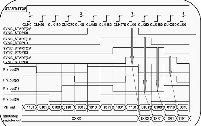
The Virtex-5 Digital Clock Managers (DCMs) provide a wide range of clock management features and allow phase shifting. I used a DCM that gives four copies of the same clock signal shifted by 0° (clk0), 90° (clk90), 180° (clk180) and 270° (clk270). The second stage is built around a state machine synchronized by the DCM output signals, used to perform a first level phase interpolation thus giving a resolution of a quarter of the clock period (about 454 ps). The third stage performs the fine time measurement thus improving the coarse counter resolution. Since I also exploit the four phases information delivered by the DCM, the fine time measurement must only interpolate in between the four different phases i.e. over a quarter of the clock cycle. I designed two different fine time converters in order to compare their performances side by side. The first one consists of tapped delay lines and the second one uses Vernier delay lines.

I used the Xilinx Integrated Software Environment 9.1 (ISE) development tool to realize the different types of TDC architectures [46]; in the design and simulation phase the VHDL (Very high speed integrated circuit Hardware Description Language) [47] has been used.

The main design problem was related to the high frequency design of the coarse TDC and to keep the linearity of the fine TDC output. These problems were solved by manually placing both logic gates and flip-flops.

(44)

3.2 Design flow and timing closure approach

The basic elements of a FPGA are the programmable logic blocks and the programmable interconnects. The logic block can perform basic (AND, OR, NOT) or complex logic functions and also includes memory elements. The programmable interconnections allow the logic blocks of a FPGA to be connected as needed by the system designer.

In Virtex-5 FPGA each Configurable Logic Block (CLB) is divided into two slices; each slice consists of 4 flip-flops, 4 6-input Look Up Tables (LUTs) and dedicated carry logic that can be used to cascade function generators in order to implement wide logic functions. These high-speed chain structures are usually used to realize fast counters, adders and multiplexing of data.

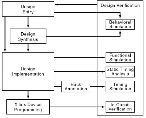
Figure 3.1 shows the standard design flow, it comprises the design entry and synthesis, the design implementation and the design verification.

Figure 3.1: Standard design flow.

My design entry is made by VHDL files. These files must be synthesized by the compilation tool into a logical design file format, i.e. a punctual description of the hardware interconnections of logic gates and flip-flops.

The design implementation begins with the mapping or fitting of the logical design file to a specific device and is completed when the physical design is successfully placed and routed and a bitstream file is generated. The propagation delays, inside the programmable device, are calculated during the

(45)

implementation procedure. This phase is called back-annotation. The physical design informations are then translated and distributed back to the logical design.

The design verification then tests the functionality and performance of the implemented logic. This task is accomplished by making the functional and timing simulations, the static timing analysis and finally the in-circuit verification. The design verification procedures take place throughout the design process. Functional simulation determines if the logic in the design is correct before implementing it in the device. Timing simulation verifies that the implementation runs at the desired speed under worst-case conditions. Static timing analysis is used for quick timing checks of a design after it is placed and routed. It also allows to determine path delays in the design. The final test of the design consists of performance measurement in the target application. In-circuit verification tests the circuit under typical operating conditions. Different iterations of the design can be loaded into the device and test it in-circuit because the device is reprogrammable.

The high speed design puts several constraints on the mapping, the placement and routing of the logic. There can be only one level of logic gate between the output and the input of several flip-flops. Logic functions that need several inputs, normally using more than one logic level, had to be pipelined between more clock cycles. This strategy increases performance at the expense of adding latency. Depending on the application, the dedicated slice carry logic can be used to provide wider logic functions.

Some flip-flops input have to be driven by logic elements inside the same slice of the Virtex-5 FPGA in order to lower the number of routing nets on the signal combinatorial paths. Figure 3.2 shows the simplified circuit block diagram of this timing closure approach; some elements of the Virtex-5 FPGA slice are omitted for clarity. The flip-flops in the slices are configured as positive edge triggered D-type.

The source flip-flops FFA and FFD are located in the slice A; they drive a LUT (Look Up Table, 6 input function generator) packed with another flip-flop FFD in a surrounding slice. The LUT is configured in order to realize a 2 inputs combinatorial function (as AND, OR, etc..). Several routing connections between the two slices are possible and the Xilinx ISE software finds the most optimal routes. All of the interconnect features are transparent to the FPGA designers that can view the delay of these nets using FPGA Editor. In order to verify the tight timing requirement of a high speed design, the routing connections Net A and Net B have to be as short as possible and with fewer hops; in fact the propagation delay of these nets have to be lower than 1 ns. The value of the maximum propagation delay of these nets is related to the slice timing parameter and is calculated in order to avoid a metastability problem of the flip-flops therein the slice.