S
Ex
Tuto
CUOLA D
xperime
Flu
or: Prof.
DOTTORA
ental In
uctuati
Roberto
ALE IN IN
nvestig
ions of
S
A
o Camuss
NGEGNER
XXIII CIC
gation o
a Comp
Silvano G
A.A. 2010
si
RIA MECC
CLO
of the N
pressib
Grizzi
0/2011
CANICA E
Near‐Fi
ble Rou
E INDUST
ield Pre
und Jet
TRIALE
essure
Index
1 Introduction ... 3 1.1 Objectives ... 5 2 Turbulent and Acoustic Jet Properties ... 7 2.1 The Turbulent Jet ... 8 2.2 Overview on the Jet Noise ... 12 2.3 The Acoustic Analogy ... 13 2.4 Recent Acoustic Theories ... 14 2.5 Sound and Pseudo‐Sound ... 15 3 Wavelet Filtering ... 18 3.1 Fourier Transform versus Wavelet Transform ... 18 3.2 Wavelet Decomposition of Sound: A novel approach ... 20 4 Experimental Setup ... 30 4.1 The Semi‐Anechoic Chamber ... 30 4.2 The Jet geometry ... 32 4.3 The Calibration of the Jet ... 37 4.4 Velocimetry and Acoustics sensors ... 41 5 Jet Characterization ... 48 5.1 The Jet Flow‐Dynamics ... 49 5.2 The acoustics of the Jet Far‐field ... 59 6 Near‐Field Pressure Fluctuations ... 69 6.1 Near‐field characteristics ... 706.3 Mach number effects ... 82 6.4 Near‐field Far‐field Correlation ... 89 7 Identification of Noise Sources ... 91 7.1 Hot‐wire interferences ... 91 7.2 Velocity‐Pressure Correlations ... 95 7.3 Potential Core Fluctuations ... 100 8 Conclusions ... 103 8.1 Future Works ... 104 Appendix A: Duct and Nozzle Design... 105 Appendix B: Far‐field Spectra ... 112 Appendix C: Near‐field Spectra ... 115 Appendix D: Near‐field, Hot‐Wire measurements ... 121 Bibliography ... 125
1
Introduction
The commercial airline industry is one of the largest global industries and affects many aspects of daily life. The air transport has a significant environmental impact on the residential zones and the continuous expansion of the urban areas near the airports makes necessary the limitations of the noise pollution. The problem of noise generation by turbulent compressible jets has been of great interest since the early 1950s with the introduction of jet engines in commercial aircraft and even later with the adoption of high by‐pass ratio turbofan engines. Since that time, considerable research activity has been undertaken to understand the generation and propagation of jet noise, as well as to devise techniques for its reduction. The noise that affects the inhabitants of the urban areas around the airports is called as Community Noise (see Figure 1) and is submitted to strictly laws; the noise that affects the passengers is called Cabine Noise (see Figure 1) and is also a critical parameter that forces a massive use of acoustic‐absorbent materials inside the aircrafts. These strict limitations bring to a more accurate investigation of the jet noise production mechanisms evolving equally theoretical, experimental and numerical aeroacoustics research. Deeper jet noise knowledge brings to the realization of less noisy aircrafts; this topic becomes also fundamental for the newest realization of aircrafts using composite materials that protects less the passengers from the noise than the metals.
The term “Jet Noise” is frequently used to describe the total noise emanating from an aircraft exhaust system; studies have shown that this total noise is composed of several parts. The most fundamental of these is due to the turbulent mixing of the jet exhaust with the ambient fluid downstream of the nozzle exit section. This “Jet Mixing Noise” is the most difficult component to control and to eliminate.
The jet mixing noise is one of the main sources of the aircraft engine total noise (see Figure 2) and it has historically received the most attention since the Lighthill’s works (Lighthill 1952
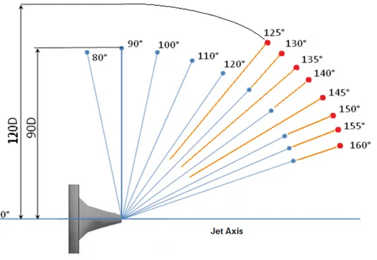
& 19 of th moti comp appr prop Figure The ment flow prese (defi As p intim unde 954). The Lig he “Aeroaco on are reca prises all t opriate to pagating sou e 1: Communi community tioned acou has the eff ents a max
ning 180° d ointed out mately relat erlying the p ghthill’s pap oustics” res ast as an in he non‐line describe th und‐field dr ity Noise distr
y noise is ustic model fect to give ximum ang downstream by Michal ted to the propagation
pers have m search area
homogeneo earities. Lig he jet noise iven by a co ribution for a s also defin ls. In the je a significan gular direct m the jet axi
ke and Fuc e hydrodyn n of acousti marked the b . In the Lig ous wave e ghthill recog
e; the flow onfined reg
single takeoff
ned as far‐ t noise the nt directivit tion, with s). chs (1975), namic velo ic waves to beginning o hthill’s ana equation, w gnized that is describe ion of inten f (Left) and Ca ‐field noise convection ty to the jet a maximum the knowl ocity fluctu the far fiel of jet noise logy the ex ith the inho t this form ed using th nse rotation bine Noise pe
e and is w n of the sou t noise. In f m direction edge of th ations, can d. However research an xact equatio omogeneou mulation is his analogy nal motion. eak region (Rig well describ urces down act, the far n around 1
e near field n clarify th r, as report nd the birth ons of fluid us part that particularly as a freely
ght)
bed by the stream the r‐field noise 140 ‐ 150° d pressure, he process ed in many h d t y y e e e ° , s y
2008), considerable efforts have been devoted to the characterization, prediction and modeling of the far‐field noise along with the attempt of relating the far field acoustics with the hydrodynamic near‐field.
Figure 2: Noise distribution on an aircraft during the takeoff (Left) and influence of the noise sources during approach and takeoff (Right): the Jet exhaust is one of the main sources during the takeoff phase.
The near‐field noise, that influences passengers’ comfort, on the contrary, seems to be different and not so well described by acoustics models for the presence of other pressure fluctuations that are not sound because they don’t have all the features of the sound. The near pressure field investigation of an unbounded jet has been the subject of a considerable number of experimental and theoretical investigations over the past 60 years to understand flow‐dynamics and sound production and propagation mechanisms. 1.1 Objectives
The main aim of this study is the investigation of the near‐field noise that is considered nowadays interesting for the possibility to locate the noise source.
To perform this investigation some objectives have been pursued: ‐ A jet noise facility has been designed and realized. ‐ The jet facility has been qualified and compared with literature studies. ‐ The near‐field pressure fluctuations have been analyzed and filtered to separate the sound contribution; to perform this, a novel filtering procedure has been developed. ‐ Synchronized measurements of velocity and acoustic fields have been carried out to locate the noise generation zones of the jet. This thesis is organized as follows:
The Chapter 2 gives an overview of the jet properties starting from the turbulent characteristics related to the jet noise production mechanisms, describing models and theories from the Lighthill’s analogy to the recent developments.
The Chapter 3 describes the analysis and filtering methods with particular attention to the wavelet‐based algorithms. This represents a novel approach in aeroacoustics studies.
The Chapter 4 presents the experimental setup and the measurement techniques used to study the jet; the used hardware is analyzed to define its application limits and to quantify its accuracy.
The Chapter 5 presents both flow‐dynamic and acoustic qualification of the jet and the results are compared with literature data.
The Chapter 6 shows the near‐field pressure fluctuations comparing the filtered and non‐ filtered data with the far‐field and with literature data.
In the Chapter 7 the identification of noise production zones is performed correlating the velocity and the acoustic data; a comparison also with some previous studies is done.
At the end the Chapter 8 presents some conclusions and suggestions for future works.
2
Turbulent and Acoustic Jet Properties
The noise produced by a jet is governed by the turbulence flow from it; the basic mechanisms involved in the jet noise production are still not understood. The complex nature of the turbulence is dependent mainly by the three dimensional character of the velocity field, its non‐linearity and its random and intermittent variation. The statistical models for the turbulence introduce simplifications that don’t allow an accurate understanding of some noise production mechanisms. In turbulence models it is impossible to predict the exact value of fluctuation at a given moment but it was accepted in the research that the average values for particular locations in the flow should remain constant; in this manner not all scales of the turbulence can be viewed. For this reason, for example, the identification of intermittent large scale structures is difficult for any time averaging analysis technique. However the statistical properties of turbulence have provided great information on the nature of a turbulent flow and are useful for the prediction of its noise generation.
A jet airflow produces pressure fluctuations either in the form of regular eddies or an irregular turbulent flow. These pressure fluctuations can be detected and measured by a microphone or the human ear; only a relatively small part of the energy of these fluctuations can be called sound. Most of the pressure fluctuations, for example eddies, are convected in the flow at the flow speed and don’t propagate at the typical sound speed. These hydrodynamic pressure fluctuations transfer a certain amount of their kinetic energy into radiated sound. An examination of the radiated sound field reveals that is comprised of a broadband spectrum so all turbulent scales must contribute to the propagating noise. However the large and small scales of turbulence may behave differently and the exact mechanisms of sound generation from these fluctuations are not yet completely understood.
A key point of the aeroacoustics research is the identification of noise production mechanisms from each turbulent structure during its evolution in the flow field. The full understanding improves the active noise control and reduction modifying the flow turbulent characteristics. The purpose of this work is to correlate the pressure fluctuations to some generation mechanisms in the flow; for this reason an introductive description of jet properties is necessary. 2.1 The Turbulent Jet A jet is a flow that enters in a stationary fluid. This interaction brings to intense mixing and creates a shear layer. Going downstream the shear layer widens through the axis of the jet; the conic zone between the exit section and the point where the shear layer meet the jet axis is the potential core; in this zone the velocity maintains constant and it is extended to a distance of 3 – 5 diameters (Rajaratnam 1976). In the potential core the axial velocity profiles starts with a top‐hat shape and evolves maintaining the maximum velocity value equal to the jet velocity, the velocity gradients between the jet core and the external fluid becoming smooth moving downstream (see Figure 3). Beyond this distance, the turbulence produced by the shear layers from the border of the jet reaches the jet centreline and dissipates the velocity; after this point a transition zone begin and changes quickly to a fully developed flow zone. The structure of a jet is shown in the Figure 4.
In the fully developed region the velocity and turbulence profiles are comparable and are known as self‐similarity profiles. In fact the velocity and turbulence radial profiles, opportunely scaled, can be perfectly overlapped as observed by Trupel (1926).
As previously mentioned the axial velocity is constant inside the potential core, so, along the jet axis, the non‐dimensional axial velocity has a constant profile until the end of the core, after that it decreases with a 1/X law (Eq. 1); according to literature the decreasing factor is usually between 5 and 7.5 (see Tab 1).
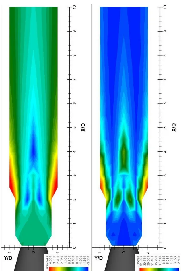
Figure 3: Potential Core velocity profiles. (Cenedese et Al. 1994) Figure 4: Structure of a Jet. The potential core end is located where the axial Kurtosis has a maximum, downstream this point the jet becomes fully turbulent and the velocity profiles became self‐similar. Many experimental data and empirical solutions are available to compare the jet profiles as Tolmien, Goertler type (Rajaratnam 1976) or Integral Solution (Agrawal e Prasad 2003).
These characteristics are useful to verify that the jet studied in the presented work has been designed correctly. Eq. 1 Reference C coefficient Trupel (1926) 7.32 Hinze Zijne (1949) 6.3 Albertson et Al. (1950) 6.39 Grizzi et Al. (2006) 7.47 Panchapakesan e Lumley (1993) 6.06 Hussein et Al. (1994) HW 5.9 Hussein et al. (1994) LDA 5.8 Grandmaison (1982) 5.43 Becker (1967) 5.59 Ebrahimi (1977) 5.78 So (1990) 5.51 Dowling (1990) 5.11 Tab 1: Axial velocity decreasing coefficients.
In the self‐similarity zone the velocity and turbulence profiles have to be scaled using as parameters the maximum local axial velocity (Um) and the half jet aperture radius (b), which
is defined as the distance from the axis where the local velocity is half of the local maximum velocity. (see Figure 5) Moreover, also the turbulence profiles are self‐similar as the axial Reynolds stress u’2 is scaled with respect to Um2 (see Figure 6).
Another important feature is the state of the boundary layer in the nozzle that, just at the exit section, can be laminar or turbulent. In this work it has been checked that the boundary layer is turbulent.
Figure Figure (1994 e 5: Dimensio e 6: u’/Um2 s 4). nal (top) and self‐ similar p non‐dimensio
rofiles: on the
onal or self‐sim
e left Weisgra
milar (bottom
aber e Liepm
m) velocity pro
mann (1998); o
files (Abramo
on the right H
ovich 1963)
2.2 Overview on the Jet Noise
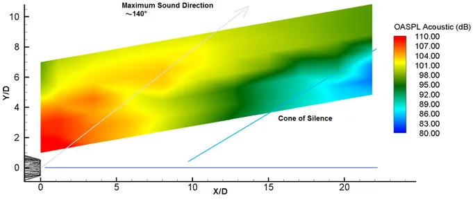
Several regions in the jet structure are interesting for the noise production but there is a lot of uncertain in the physical mechanisms of noise production. In the Lighthill’s works (1952 and 1954) the sources were modelled as freely‐convected quadrupoles; during the 1970s large scale structures were discovered in the shear layer and this structures’ noise production were studied. Juvé (Juvé et Al. 1980) shows that these structures have a significant intermittency; he demonstrates also that the 50% of the noise is produced in the 10 – 20% of the total time. Juvé suggests also that the noise emissions can be placed also upstream of these structures where the external fluid was entrained. It has been shown that the breakdown of the structures at the end of potential core is a significant mechanism of noise emission (Guj et Al. 2003, Hileman et Al. 2005) There are other phenomena that affect the noise radiation from the sources in the jet; the noise sources are convected in a high speed flow affecting the directivity of the radiated noise. In addition the noise must pass through the shear layer and suffers of refraction effects by the velocity gradients generating the well‐known “cone of relative silence” (Tanna 1977). Other characteristic of the noise is the different spectral content as a function of the direction. Tam et Al. (1996 and 1999) proposed that the fine‐scale turbulence is responsible for the noise at 90° and the large scale structures generates the noise at 150°, defining 180° direction as the jet axis downstream; other researchers explained on the contrary the different spectral contents in the far‐field as a different directivity that affects different scale sources.
2.3 The Acoustic Analogy
The Lighthill’s Acoustic Analogy was developed in the early 1950s (Lighthill 1952 – 1954); this works represents the beginning of aeroacoustics science and allows to made acoustic predictions of turbulent flow for the first time. In the Lighthill’s work a small part of the fluid is occupied by the main flow that generates fluctuations, the rest of the fluid is only interested by the acoustic propagation. Lighthill recasts the exact equations of fluid motion in the form of an inhomogeneous wave equation, whose inhomogeneity comprises all the non‐linearities of the Navier‐Stokes equations. This equation describes freely propagating linear disturbances which are driven by the dynamics described by a non‐linear term on the right‐hand side (Eq. 3).
Eq. 3 Lighthill recognised that this form is particularly well suited to the problem of the jet noise where the system is divided in a freely propagating sound field, which is driven by a confined region of intense rotational and non‐linear motion. The right‐hand side term is the Lighthill tensor (Eq. 4) that incorporates sound generation, convection with the flow, propagation with variable speed and dissipation by conduction and viscosity (Lighthill 1952). Eq. 4 From the previous equation, considering that the viscous dissipation is a very slow process and that the static pressure field variation is negligible in problems where the temperature is fairly uniform, the principal terms of sound generation are the Reynolds stresses . The modelling of this term in the Eq. 3 is one of the targets of the research. A model proposed by Ribner (1964) assumes homogeneous isotropic turbulence and the sources as a distribution of freely‐convected quadrupoles with strength related to the two point correlation function of the Reynolds Stress; this requires detailed turbulence statistics to perform an accurate
take into account the changes in radiation efficiency due to the interaction of the flow environment and the sources. Several new models and modifications to the Lighthill analogy were proposed during the years. 2.4 Recent Acoustic Theories One of the most popular of this model is the one proposed by Tam and Aurialt (1999) and relates the local turbulent kinetic energy to the local pressure fluctuations of the small scale turbulence. This model is semi‐empirical and relates the noise to the fine scale turbulence and not with the large scale structures. For this reason the two sources theory was subsequently introduced and attributes different spectral directivities to different sources. All the presented models from the Lighthill or the Lilley approaches regard the small‐scale component but only recent studies identify also large‐scale mechanisms that generate pressure fluctuations. Coiffet et Al. (2006) shown experimentally the existence of vortex‐ pairing and wavy‐wall type instabilities in the region upstream the end of the potential core and demonstrate that the production mechanism is linear. Kopiev and Chernyshev (1997) have provided an analytical demonstration of how the eigen‐oscillations of a single vortex structure can constitute an octupole sound production mechanism, which presents directivity similar to the jet (Kopiev et A. 1999, 2006). There are also many studies that indicate as dominant sound production mechanisms the intermittent and violent collapses of the annular mixing layer at the end of the potential core. Juvé et Al.(1980) shown that the events in this region have high level of intermittency: the possible mechanisms are identified as the sudden decelerations near the end of the potential core, related to fluid entrainment on the upstream side of ring‐like coherent structures. Other works as Guj et Al. (2003) or Hileman et Al. (2006) provided other experimental evidences for this sound production mechanism.
have a quadrupole behaviour; the other is related to the coherent flow dynamics, which can produces sound via‐vortex pairing, vortex eigen‐oscillations, quasi‐irrotational instability or wavy‐wall‐like mechanisms and intermittent events in the transition region of the flow. Is unclear how the two mechanisms contribute differently to the sound directivity. Probably an angle‐dependent frequency selection occurs depending by the interaction between the sound field and the flow dynamics.
2.5 Sound and PseudoSound
The main objective of aeroacoustics is the comprehension of the physics of noise generation; the uncertain in the real noise sources contribution needs more experimental studies, for this reason many tests were conducted to locate the sources and the noise generation mechanisms; to accomplish the velocity information and sound measurement are correlated both in far‐field and in near‐field. As previously mentioned the near‐field measurements, which are more useful for the sources localization, are affected by some‐pressure fluctuations that are not sound. Howes (1960), Ffowcs‐Williams (1992) and Ribner (1964) describe the presence of pressure fluctuations, called pseudo‐sound, in the near‐field that are not sound but are undistinguishable, using a microphone, from the sound. In fact, when sound is generated by an unsteady flow, only a small part of the energy associated with pressure fluctuations radiates as sound and the main pressure fluctuations masks sound field near the jet. A filtering method to separate sound from pseudo‐sound is necessary to compare the far‐field with the near‐field noise and it is also useful for noise‐control applications.
Ffowcs‐Williams (1992) wrote:
”It is only when the pressure satisfies this equation (Equation of the waves) that it is properly regarded as sound. Other pressure fluctuations, indistinguishable by a single microphone from proper sound, have been termed Pseudo Sound, only pseudo because they lack some essential characteristics of sound. They do not propagate through the fluid but are convected
with the eddy structures in the flow, often in chaotic path and usually with a speed very much smaller than the sonic velocity.”
The pseudo‐sound is convected with eddies, it is the rotational part of the flow and do not propagate. Instead, the sound propagates but it is negligible when the pressure field is dominated by the pseudo‐sound. The pseudo sound field decays very rapidly, usually with the inverse of the third power of the distance, and, at large distances, the pressure field reduces to the acoustics field (Howes 1960).
In the flow region, the pseudo‐sound is the quasi‐incompressible pressure fluctuations part and it is dominated by inertial effects rather than compressibility. Pseudo‐sound is a solution of the Poisson’s equation (Ribner 1964).
The sound is also present in the near field region, is described by wave equation and it is the irrotational part of the pressure field. When a measure is performed in the near‐field the acoustical contribution is affected by the hydrodynamic one since a microphone is subjected to fluctuations both of the sound and of the pseudo‐sound (Howes 1960).
Considering the different nature of the two parts an important task for a near‐field measurement is the filtering of the two contributions from a near field signal. The pseudo‐ sound is associated to the convection of structures through the flow and for this reason carries information about the coherent structures. The remaining part is the sound and it is associated to the incoherent part of the pressure fluctuations. Ribner (1964) divides the pressure fluctuations p’ into sound (p’0) and pseudo‐sound (p’1) fluctuations:
Eq. 2
Also in Guitton et Al. (2007) the near pressure fluctuations of a jet are considered as a superposition of sound and pseudo‐sound fields. When possible a filtering operation can divide the pressure fluctuations in the two contributions that, for the different nature of them, have different behaviours as the different propagation characteristics. Usually Fourier’s based filters are used to distinguish the two parts but this is not efficient because, for its nature, this filtering is equivalent to a high‐pass and low‐pass filtering, in fact the
(2008) the acoustic‐hydrodynamic filtering is performed starting from microphone array measurements and calculating the phase velocity of the signal on the array because “no
sound field can produce a subsonic phase velocity” (Tinney and Jordan (2008).
Considering that sound and pseudo‐sound may have energy to the same frequencies and filtering only in the frequency domain is not sufficient for a complete signal splitting. For this reasons a Wavelet filtering tool is more indicated, the Wavelet transform is located both in the frequencies both in the time domain (Graps 1995) and the signal splitting is possible considering the intermittency of events; in fact, using the wavelet, is possible to separate the intermittent events from the rest of the signal; the coherent structures pass through the microphone at intermittent intervals and the remaining signal is related only to the acoustic field. It must be remembered that the intermittent nature of the large scale structures in the velocity field is a noise generation mechanism (Juvé et Al. 1980; Tinney and Jordan 2008) but the intermittent nature of pressure fluctuations in the near‐field is related on the contrary to the convection of the large scale structures and its nature is different by the sound, as will be demonstrated in the next chapter.
3
Wavelet Filtering
Classical statistical tools assume to have a homogeneous flow without discontinuities or intermittent events; a wavelet‐based tool does not require such hypotheses. Wavelets are mathematical functions that cut up data into different frequency components, and then study each component with a resolution matched to its scale. They have advantages over traditional Fourier methods in analyzing physical situations where the signal contains discontinuities and sharp spikes. Wavelets are functions that satisfy certain mathematical requirements and are used in representing data or other functions, expanding or contracting the selected wavelet, also called mother wavelet, using an opportune scaling function, the algorithm can analyze the data both in time both in frequency domain and obtain the wavelet coefficients. The analyzed signal can be represented as a linear combination of the mother wavelet with these coefficients. Selecting an opportune threshold the original signal can be also divided in two parts obtaining two signals: one with the coefficients greater than the threshold and the other with coefficients lower than the chosen value (Graps 1995). Moreover the wavelet analysis locate the intermittency of events (Ruppert‐Felsot et Al. 2009) and makes possible to separate the time history of these events from the rest of the signal. In turbulence the wavelet are successfully used for the identification of intermittent structures analyzing the velocities or the pressure fields, as in the works of Lee and Sung (2002) or Camussi et Al. (2008 and 2010).
3.1 Fourier Transform versus Wavelet Transform
The Fourier and the Wavelet transform have similar aspect, for example both decompose the signal in basis functions, that are sinus and cosines for the Fourier transform and the
coefficients of the basis functions but the Fourier transform give only a description in the frequency domain (the windowed Fourier transform gives also a description in time domain but maintaining a uniform resolution as shown in Figure 7) on the contrary the wavelet transform, using very short‐in‐time functions and scaling them, decomposes the signal both in frequency both in scale domain. The wavelet transform in fact, with respect to the Fourier transform or the windowed Fourier transform, uses functions localized in space and this feature gives the possibility to describe the signal with a resolution that depends by the scale length of each event (see Figure 7). So the wavelet can isolate the discontinuities using very short basis functions and at the same time can offer a detailed frequency analysis using very long basis functions. These characteristics made of the wavelet transform the perfect tool to analyze signals that present intermittent or random events with discontinuities indicating also when a single event occurs and which frequencies or length scales it involves.
Figure 7: Time‐frequency differences of the Windowed Fourier Transform (left) respect to the Wavelet Transform (right) (from Graps 1999)
Another difference is that the Fourier transform uses just sinus and cosines functions instead the wavelet has an infinite set of basis functions (see Figure 8).
In details the wavelet transform decomposes the signal in a set of coefficients resulting from the projection of a signal onto a basis of compact support functions (Eq. 3); the basis is composed by stretched (r) and shifted (t) versions of the mother wavelet Y.
, ⁄ ⁄ Eq. 3
This decomposition leads to a description of the signal both in time and in frequency domain. Figure 8: Example of wavelet mother functions: Coiflet 3 function (left) and Daubechies 6 function (right). 3.2 Wavelet Decomposition of Sound: A novel approach
The nature of the near‐field pressure measurements, for the presence of the sound and pseudo‐sound components, requires the development of a filtering algorithm that recognizes intermittent and random events separating them from the rest of the signal. As previously described the intermittent events are related to pressure fluctuations caused by coherent convected structures so there is the possibility that this part of the signal has a pseudo‐sound nature; on the contrary the remaining part of the signal, that represents the incoherent part, could be only composed by sound. The verification of these hypotheses is a
fluctuations is performed calculating the cross spectra and the phase velocities (Tinney and Jordan 2008) but a Fourier based method can’t capture all the frequencies of intermittent and random events because this filtering method is similar to a pass‐band filter; on the contrary the sound and pseudo‐sound can exist at the same frequencies with different energies and the wavelets are the best tool to perform this filtering.
An orthogonal discrete wavelet transform is used to separate the coherent intermittent events from the rest of the signal and a verification of the correct threshold value is performed considering the different properties of which can be considered as sound and which is only pseudo‐sound; in fact, an intermittent event is properly chosen when its LIM exceeds a threshold value because it is proportional to the energy of the event (Graps 1999). The main algorithm is presented by Ruppert‐Felsot et Al. (2009), the algorithm used to separate the coherent structures from the rest of the signal in a sort of de‐noise filtering. In this algorithm the threshold, as demonstrated in Donoho & Johnstone (1994), to remove an additive Gaussian white noise is proportional to the variance of the noise [Eq. 4].
The variance of the noise in not known a priori, the first step threshold is set proportionally to the variance of the full signal [Eq. 4]. The signal is divided in a coherent and incoherent part using this threshold; the coherent part is described by the wavelet coefficients that exceed the given threshold. The next step threshold is evaluated using the variance of the incoherence part at the current step; the algorithm iterates until the wavelet coefficients became constant.
2 Eq. 4
is the variance on the incoherent signal at the n‐pass, and N is the resolution of the signal acquisition. The time history signal of the coherent structures is obtained from the inverse wavelet transform of the coefficients that exceed the selected value; the rest of the total wavelet coefficients compose the noise part of the signal. To distinguish the coherent structure pressure fluctuations from the others in the near field is necessary to verify if the coherent and the incoherent signals has sound characteristics. A useful way to distinguish if a particular signal can be considered as sound or not is to verify its propagation velocity
(Tinney and Jordan 2008); to calculate the propagation velocity is necessary to have at least two contemporary signals from different measurements points with a known distance. The cross‐correlation of this signal gives the elapsed time of a fluctuation between the two points and consequently the propagation velocity. A couple of microphones is put in the near‐field, aligned with a known distance and with an angle respect to the jet axis to maintain parallel to the jet shear layer. Some measurements of the near‐field pressure fluctuations can demonstrate such hypotheses on the sound and pseudo‐sound; the filtering algorithm (Ruppert‐Felsot et Al. 2009) is applied to this signals and each signal gives back two time histories for the coherent and the incoherent part. The cross‐correlation of the parts of the signals from the two microphones verifies that the propagation velocity of the coherent part is lower respect the sound speed; instead the propagation velocity of the incoherent part is sonic or supersonic when the sound wave propagation direction isn’t parallel to the microphones alignment (see Figure 9). From the cross‐correlation is easy to calculate the propagation velocity of the incoherent signal (e.g. Figure 9):
0.014
3 10 466 /
t is the time lag between the time origin and the first correlation peak. The propagation velocity is greater than the sound speed as an effect of the misalignment of the wave propagation respect to the microphones axis and this is a first clue that the incoherent signals are sound. Making the same calculation for the coherent correlation time, it is obtained:
0.014
9.4 10 149 /
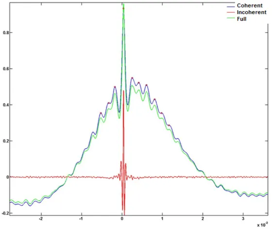
This propagation velocity is lower than the sound speed (Tinney and Jordan 2008) and indicates that the coherent part of the signal is convected in the flow; we can consider it as Pseudo‐Sound. The Figure 9 shows also the shape of the correlation functions, the coherent part has a correlation similar to the full signal part, and it means that in these measurement positions the pseudo‐sound has a lot of energy; the shape of the blue line is large and has
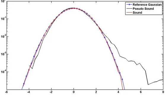
the incoherent part (the red line) the peak is very thin with a similar Dirac shape with strong oscillations around the main peak, this is a typical characteristic of this part of the signal. A further verification is possible comparing the probability density function of the <sound; incoherent> signal and of the <pseudo‐sound; coherent>; as shown in the Figure 10 the pseudo‐sound is asymmetric and has tails, is the PDF of coherent structures (Ruppert‐Felsot et Al. 2009); on the contrary the PDF of the sound is very close to a perfect Gaussian distribution (Frisch and She 1991). The differences of the coherent and the incoherent signal are evident and indicate two different natures. The coherent pressure fluctuations have a typical convective velocity and the incoherent propagate with sound speed. This briefly described algorithm is efficient when the coherent part of the signal (or pseudo‐sound) has more energy than the incoherent one (see Figure 9); these conditions are present in the zone nearest to the jet shear layer.
Figure 9: Cross correlation of the two microphones: Full signal (green line), Coherent part (blue line) and Incoherent part (red line)
Figure 10: PDF of Sound and Pseudo‐Sound part of a wavelet filtered signal.
However the energy of the pseudo‐sound decreases rapidly (Howes 1960) and the algorithm loses efficiency when Sound and Pseudo‐Sound start to have comparable energies (see Figure 11). The Figure 11 shows the use of the base algorithm in this particular condition. The algorithm is unable to separate all the incoherent part from the coherent indeed, the coherent signal still contain an incoherent part as evident from the shape of the correlation function that is a combination of a Dirac and a large Gaussian function.
Also the PDF of these signals indicates an inefficient filtering. As shown in Figure 12, both the coherent and the incoherent part are very close to the reference Gaussian. In this critical case the proposed algorithm underestimates the correct threshold, thus a modified version of the algorithm has been applied. In the new algorithm the threshold value is iterated. At each iteration the cross‐correlation is computed and the iterations end when the correlation shapes, the PDF of the signals and the convective and the acoustic velocities confirm that is obtained an optimal filtering of Sound and Pseudo‐Sound. The previous described algorithm is used for a first threshold calculation in a prediction phase.
Figure 11: Cross correlation of the two microphones in a critical zone: Full signal (green line), Coherent part (blue line) and Incoherent part (red line)
Calling the signal from the i‐microphone as Si, Sci is the coherent part of this signal and Sii is
the incoherent part. The modified algorithm controls the correlation functions of coherent and incoherent parts of the signals. The applied wavelets are orthogonal, so:
Si= Sci + Sii Eq. 5
The correlation for coherent structures (Sc1‐Sc2) is large, similar to a Gaussian function
around the peak and its peak position is proportional to the convective velocity.
The correlation for incoherent signals (Si1‐Si2) is quite similar to a Dirac function and the peak
position is proportional to the sound velocity propagation. This substantial difference between the two peaks makes possible to select a correct modified threshold until the two correlation functions (Sc1‐Sc2 and Si1‐Si2) assume the right shapes (e.g. Figure 13). At each
iteration the algorithm calculates both the convective and the sound velocities and the signal to noise ratio (SNR) of the correlation functions. The SNR is overestimated as the ratio of the first and the second peak of the correlation functions. The algorithm ends when the convective velocity is subsonic, the SNR is greater than an appropriate value and the coherent PDF divergences from a reference Gaussian function but only if the incoherent PDF remain close to the Gaussian. The Figure 13 shows an example of correct cross‐correlations.
With the use of the modified algorithm the PDF of the coherent signal becomes asymmetric with tails and the incoherent PDF maintains the Gaussian shape as shown in Figure 14; in this case the calculated propagation velocities from the Figure 13 are Vc = 55 m/s for the
coherent signal and Vi = 410 m/s for the incoherent.
Another control is performed “a posteriori” with the cross‐correlations Sc1‐Si2 and Si1‐Sc2, to
verify the independence of the sound from the pseudo sound signals. If the filter is efficient, this cross‐correlation is minimized (see Figure 15). Figure 14: PDF of the filtered signals with a well selected threshold. In this chapter a wavelet approach was proposed, a filtering algorithm and its evolution are applied for some near‐field measurements and their limits were tested. Starting from two signals of pressure fluctuations acquired in the near‐field, the algorithm divided them in two parts, the coherent part, that is the intermittent part of the signal, shown convective propagation velocity and characteristics that are related to the pseudo‐sound pressure fluctuations. On the contrary the incoherent part propagates with sound speed and shows characteristics of the sound field.
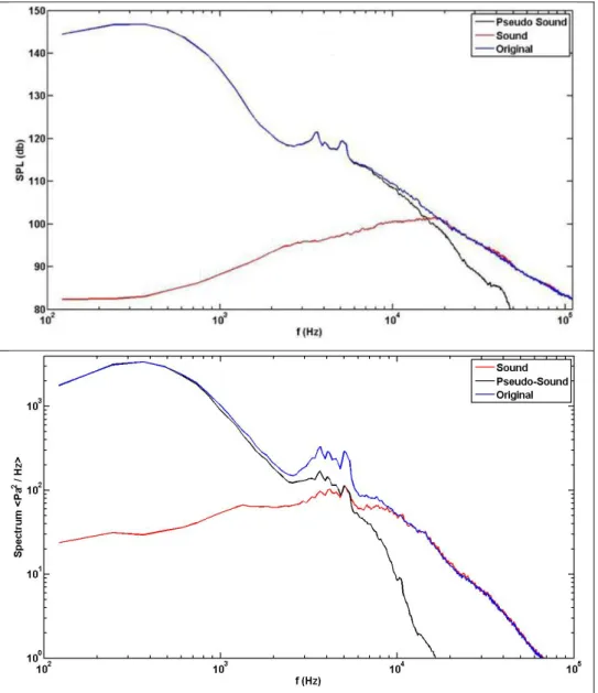
Figure 15: Verification of the independence of the sound signals from the pseudo‐sound signals: the blue line is hidden by the red one. The case where the original algorithm is efficient is shown in the Figure 16 top; is evident as the Sound spectra has very low energy respect to the pseudo‐sound. On the bottom of the Figure 16 is shown the second case after the application of the modified algorithm, the energy of the sound part is higher than the previous case. In the Figure 16 is evident as the pseudo‐sound and the sound exist in the full frequency domain and this filtering capability is only dependant by the wavelet use. A wavelet useful characteristic is that maintains the original synchronization in the inverse transformed signals, because it analyzes the signals also in time domain; it is just this feature that allows obtaining the propagation velocities of the filtered signals.
Figure 16: Filtered near‐field spectra of the pressure fluctuations: on the top a measurement point at 1 diameter from the jet shear layer; on the bottom a point at 3 diameters from the shear layer.
4
Experimental Setup
To perform correct measurements a semi‐anechoic chamber was prepared; the jet, installed in the chamber, is connected to a compressed air circuit powered by a rotary compressor. The complete setup is described in this Chapter as follows: ‐ semi‐anechoic chamber characteristics; ‐ jet duct and nozzle design; ‐ sensors and jet calibration; ‐ instrumentation; 4.1 The SemiAnechoic Chamber The setup was prepared in a semi‐anechoic chamber; the walls and the top of the room are covered with sound‐absorbent panels mounted on wood struts; during the tests also the main part of the floor, the jet and the struts are covered with the same panels and a draining space is provided in the wall in front of the nozzle to eject the air excess (see Figure 17 for a scheme of the chamber and the jet installation). A jet usually has high entrainment and engulfment mechanisms that increase the ejected air‐mass flow from the room, for this reason a recovery of the air comes from holes in the walls and from the air‐circuit on the ceiling, these air intakes are behind coating panels. Upstream of the jet duct some security valves are applied on the air‐circuit and a pressure regulator provides the correct air flow. The used nozzle has a diameter of 12 mm and for this reason generates sound at high frequencies. The used sound‐absorbent panels are composed of 100mm polyurethane pyramids having a cut‐off frequency of about 500 Hz (see Figure 18) that is sufficient forthese measurements. Moreover the absorbent coefficient at 250 Hz is 0.6 and this offers a good sound softening also at low frequencies.
Figure 17: Plant of the semi‐anechoic chamber with some dimensions (left). Jet installation in the semi‐ anechoic chamber (right) with sensors, hot‐wire and near‐field microphones.
4.2 The Jet geometry
To connect the nozzle to the compressed air circuit a duct was designed; the duct has to reduce turbulences and asymmetries coming from the air supply, and it has to prevent undesired noise propagation inside it.
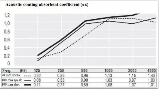
Upstream of the duct is installed a muffler (see Figure 19) that has been designed to dissipate the undesired noise produced by the valves and the compressed‐air circuit. This muffler is a reactive‐dissipative model called “lined plenum chamber” (Bell 1994). The frequency fading curve is reported in Figure 20, the coating in the installed muffler having a thickness of 100 mm. Figure 19: Reactive‐dissipative muffler: “lined plenum chamber” type. The main duct is connected with the muffler. Inside the duct is reasonable to consider the air speed lower than 10 m/s also at transonic jet velocity so is possible to dissipate the
turbulence, generating very low scale structures, without significant pressure losses or unwanted noise generation. Figure 20: Noise fading curve for different thickness of the absorbent coating. Figure 21: Duct exploded rendering.
The duct design is shown in the exploded rendering of Figure 21: it starts with a strong divergent part (part [A]) that connects the compressed air circuit (2 inches of diameter) with the rest of the duct (80 mm of diameter); in the divergent [A] there are the inlet of the main air supply and a small inlet of seeding for further velocimetry measurements; a glass wool is also inserted to eliminate noise propagation from the upstream ducts. The [B] part is a holed plate with 158 holes of 3 mm diameter each. The total area is about 10 times greater that the nozzle outlet section; this part generates small scale structures that decay in a length of 100 diameters. This system uniforms the flow and reduces the turbulence coming from the air supply and from the divergent [A]. To ensure the complete decaying the [C] duct is 30 cm of length; the [D] section contains honey‐comb of hexagonal 1 cm mesh size and 6 cm length. The honeycomb prevents swirl motions inside the flow canalizing the air in small straight ducts. At the end of the [D] section a net with a mesh squared size of 2 mm x 2 mm is placed: the net has the same function as the holed plate and generates small scale structures that decay in 20 cm of length. The main requirement for the net is the porosity ratio to be higher than 60% of the main duct. Using the Eq. 6, the porosity for the used net is Pn = 64%. Figure 22: Net geometric characteristics.
Referring to the Figure 22 the net can be divided in elementary meshes so the complete area is h2 and the empty section is d2. From geometric considerations h d 2 t/2, where t is the wire thickness. In the present case d = 2 mm and t = 0.5 mm.
100 100 Eq. 6
Downstream of the net there are [E] and [F] ducts with a total length of 20 cm; the end section of the [F] part is built to match accurately with the nozzle avoiding steps or misalignments. In this section 4 holes of 1 mm are used to place pressure transducers and thermocouples. These sensors are used to calculate the exit velocity from the flow property in the upstream part. The small diameter of these holes doesn’t interfere with the flow. At the end of the duct is inserted the nozzle (see Figure 23), having an inlet section diameter of 80 mm (d0) and an outlet section diameter of 12 mm (d); the contraction ratio is
/2 ⁄ /2 44.44. Figure 23: Axial section of the nozzle. The nozzle is designed following the specifications of Glushko (1935) (see Figure 24), where
radius, Θ is the nozzle angle, l0 is the length of the subsonic region and r is the outlet section radius. These parameters have to follow the constrains of Eq. 7 to avoid flow detachments: Θ 40° Eq. 7 Following these relationships and minimizing the l0 to avoid an excessive boundary layer at the outlet section, the nozzle is designed with values shown in Tab 2. r0 40 mm r 6 mm R1 80 mm R2 7.2 mm Θ 30° l0 82.75 mm Tab 2: Nozzle design parameters. Figure 24: Nozzle design profile (Glushko 1935). The complete Nozzle design is reported in Appendix A.
4.3 The Calibration of the Jet
As previously mentioned the jet was calibrated using the information thermocouples and pressure transducers placed just before the inlet section of the nozzle.
4.3.1 The Thermocouple
A J‐type thermocouple is used for measuring the air temperature inside the duct. A thermocouple is composed by two wires of different metals in the hot junction that represents the measuring part. A J‐type thermocouple is used. Usually the circuit of a thermocouple needs a cold junction and a voltmeter (see Figure 25), in the used sensor both the cold junction and the voltmeter are inner the Yokogawa DL708 oscilloscope that contains also the calibration function. The J‐type (iron–constantan) has a restricted range of temperatures (−40 to +750 °C), but high sensitivity of about 55 µV/°C. The Curie point of the iron (770 °C) causes an abrupt change in its characteristics, which determines the upper temperature limit.
Figure 25: Example of thermocouple measuring circuit.
The h 1 mm temp temp 4.3.2 At th press conn press the a be ca Figure As sh the v the u hot junction m of height perature of perature va 2 The Pres he same sec sure of the nected with sure limit o atmosphere alibrated to e 26: Pressure hown in Fig voltage out used transd n has a sph t therefore the air but lue as well. ssure transd ction of the section fro h an ICSens of 50 psi; it e; this trans o correlate t e transducer c ure 26 ther put: ucer. erical head its interfer t for the low ducer thermocou om small ho sors pressu gives the d sducer is po the output v calibration. re is a linea ; with a radi rence can b w velocity in uple is appli oles that do ure transdu difference owered wit voltage to t r correspon in Tab 3 ar ius of 0.5 m be neglecte n the duct ied a circuit on’t interfer cer. The u between th h constant he measure ndence betw re presente mm that is in ed. This hea it can be co t of tubes th re with the sed transd he measurin voltage DC ed pressure ween the m ed the calib nserted in t ad measure onsidered a hat capture flow; these ucer has a ng point pr C current an e (see Figure measured pr bration para the flow for es the total as the static es the static e tubes are maximum ressure and nd needs to e 26). ressure and ameters for r l c c e m d o d r
a 10.0069 Psi/mV b ‐10.1937 Psi Sensitivity 99.9 mV/Psi Uncertain <0.05% Tab 3: Pressure transducer calibration parameters. 4.3.3 Jet Velocity Calibration
The jet calibration starts from the measurement of the temperature and the pressure upstream of the nozzle. Defining A as a section, T the temperature, P the pressure and M the Mach number, the subscript i indicates the inlet section and j the outlet. The isentropic equations in an almost one‐dimensional model are:
·
Eq. 8·
·
Eq. 9
Eq. 10
Dp is obtained from the pressure transducer and Pi is assumed to be the atmospheric
pressure under the fully expanded jet hypothesis. Therefore:
Eq. 11
From Eq. 10 and 9, H and Tj are obtained; knowing the contraction ratio ⁄ from Eq. 8
and the second part of Eq.9 the outlet Mach number Mj is calculated. From Tj and Mj the
velocity of the jet is calculated using the following equation:
Figur evalu depe nozz the d guar caus Figure outpu re 27 show uated jet M ends by the le. From the duct: as sh antees that ed by the n e 27: Jet Calib ut. ws the jet c Mach numb exit tempe e previous m own in Figu t the noise
et and the
bration: Jet Ma
alibration r ber and the erature decr mentioned ure 28 the e generated honeycomb ach number ( results, the e jet exit v reasing with equations i velocity is d inside the b are very lo blue line) and pressure t velocity. Th h the increa is also poss less than 5 e duct is ne
ow. d Jet velocity ( transducer e divergen asing of the ible to eval 5 m/s, as e egligible an (red line) resp output rela ce of the t expansion uate the air expected; th nd the pres
pect the transd
ated to the two curves ratio in the r velocity in his velocity sure losses ducer voltage e s e n y s e
Figure 4.4 Durin tube veloc self‐s veloc and phen 4.4.1 The for t conn calib e 28: Evaluatio Velocim ng the expe and a hot city profiles similarity o city and tur pressure nomena. Tw 1 The Pito Pitot tube c he static p nected with ration para on of the air v metry and erimental ca t‐wire prob s both in the f the veloc bulence dis measurem wo micropho t Tube consists of ressure me a pressure meters are velocity in the d Acoustic ampaign co be were us e potential city profiles stribution a ments were ones Brüel & a small pro easurement transducer slightly diff duct with res cs sensors onducted to sed. The Pi core and in . The hot‐w long a symm e carried & Kjær 493 obe of abou (see Figur r of the sam ferent and a spect to the Je s o qualify the tot tube is n the fully d wire probe metry plane out to in 9 are used f ut 2 mm of e 29). The me model as are reporte et Mach numb e flow‐dyna s used for eveloped re is used for e of the jet. vestigate for the pres f maximum Pitot tube s the one pr d in Tab 4. ber. amic of the a qualificat egion and to r deeper st Synchroniz the noise‐ ssure measu diameter a total press reviously de jet, a Pitot tion of the o verify the tudy of the zed velocity ‐generation urements. and 6 holes sure duct is escribed; its t e e e y n s s s
a 10.04976 Psi/mV b ‐8.310 Psi Sensitivity 99.5 mV/Psi Uncertain <0.06% Tab 4: Second pressure transducer parameters. 1 Eq. 13
To evaluate the maximum interference of the Pitot tube with the flow, an additional jet calibration has been performed to evaluate the jet velocity both with the Pitot tube in correspondence of the outlet section and the sensors upstream of the nozzle.
Figure 29: Pitot tube drawings.
The interference of the Pitot tube with the flow is shown in Tab 5. The maximum interference is of about 4.7 % obtained in correspondence of the centre of the nozzle outlet section. The evaluated intrusiveness is reasonably low and the simplicity of use and robustness of the Pitot tube justify its use for a velocity qualification in terms of mean
Jet evaluated velocity Pitot tube measured velocity % error 185.8 m/s 190.8 m/s 2.7 166.2 m/s 174.1 m/s 4.7 140.3 m/s 146.2 m/s 4.3 Tab 5: Evaluation of the interference of the Pitot tube. 4.4.2 The Hot‐Wire Probe
For advanced and accurate velocity measurements a Dantec 55P11 hot wire probe (see Figure 30) is used. This probe is a single wire sensor whose characteristics are shown in Tab 6. Due to the small diameter of the wire and of the prongs, the sensor interference with the flow is negligible. The interference with the acoustic measurements will be evaluated afterwards.
Figure 30: 55P11 Hot‐wire sensor (www.dantecdynamics.com)
The hot‐wire calibration is performed using the same jet, and the information from the sensors upstream of the nozzle are used to determine the exit velocity. The probe to be calibrated is positioned at the center of the jet section and in the potential. The hot‐wire probe is used in constant temperature mode and it is calibrated starting by the lowest stable velocity generated with the jet and is extended to the necessary Mach number; a 4th order polynomial curve (see Figure 31) is generated with a least square algorithm as the best approximation for the hot‐wire voltage‐velocity equation (Eq. 14).
Tec Med Sen Sen Sen Tem Max Max Min Max Freq Freq Tab 6 Figure hnical data dium nsor materia nsor dimensi nsor resistan mp. Coeff. o x. sensor tem x. ambient t n. velocity x. velocity quency limi quency limi : Hot‐wire sen e 31: Hot‐wire for miniatu al ions nce R20 (app of resistance mperature temperature it fcpo (CCA it fmax (CT nsor characte e calibration d
ure wire sen
prox) e (TCR) α 2 e A mode, 0 m TA mode) ristics. data and the 4 nsor Dantec 20 (approx.) m/s) 4th order polyn 55P11 Platinu 5 µm nomial curve. Air um-plated t dia. 1.25 m 3.5 Ω 0.36%/°C 300°C 150°C 0.05 m/s 500 m/s 90 Hz 400 kHz tungsten mm long C
Usua dens meas seco the h from value Figure Figur comp from num 0.00062
ally the hot sity fluctua surements nd test is p hot‐wire pro m mach 0.1 es diverge f e 32: Evaluatio re 32 show pressibility m the fitting ber of 0.85 0.0275 ‐wire probe ations of of this wor performed t obe, in the to Mach 1 from the 4th on of the com ws the hot‐w can be esti g curve. Thi . 54 0.58
e can be in a transoni rk are perfo to evaluate same posit 1. The com h order equa mpressibility ef wire voltag mated to b is happens 8104 5 nfluenced b ic flow (H ormed at a e where the ion as in th pressibility ation. ffects on hot‐w e output in be importan at a veloci
5.85316
by the comp Horstman a maximum m e compress e previous effects are wire. n a wide ra nt where th ity of 280 m 21.84032 pressibility and Rose mach numb ibility effec calibration, e evaluated
ange of velo e acquired m/s that co 2 Eq and the pr 1975). Th ber of 0.6. H cts appear. , is tested a d when the ocities. The data have orresponds q. 14 ressure and he velocity However, a In this test at velocities e measured e effects of a deviation to a Mach d y a t s d f n h
4.4.3 The Microphones
The microphones used for the pressure field measurements are two Brüel & Kjær 4939 (see Figure 34). These ¼” diameter microphones are pre‐amplified to guarantee a more stable sensitivity with the temperature. They are connected to the B&K Nexus 2690 that is a signal conditioner and amplifier. The microphones have a wide frequency response up to 100 kHz (see Figure 33). The Nexus filters the signals with a band‐pass of 20 Hz ‐ 100 kHz. Tab 7 shows the characteristics of these microphones taken from the B&K product information. As shown in Figure 34 these microphones have a protective grid that has to be removed for accurate acoustics measurements according to the literature (Viswanathan 2009). Figure 33: Frequency response of the B&K microphones without the protective grid. Sensitivity 4 mV/Pa Frequency range 4 Hz – 100 kHz Dynamic range 28 – 164 dB Temperature Range ‐40°C – 150°C Tab 7: Brüel & Kjær 4939 microphone characteristics.
The respo and respo The t with Figure the rig simultaneo onse. For th comparing onse differs thermocoup a Yokogaw e 34: A Brüel ght the inner
ous use of his reason a the spect s with a max ple, pressur wa DL708E w & Kjær 4939 structure of t two microp a measure i ral respons ximum perc re transduc with a samp microphone: he microphon phones ma s performe se in 1/3 o centage diff ers, microp ling frequen : on the left t ne. akes necess d with this octave‐band ference of 1 phones and ncy of 500 k the micropho
sary to com two sensor ds. The Fig 1.5%. the hot‐wir kHz to obta ne connected mpare their rs in the sam gure 35 sho re signals ar in 5*106 sa d with its pre‐ r frequency me position ows as the
re acquired mples. ‐amplifier; on y n e d n
5
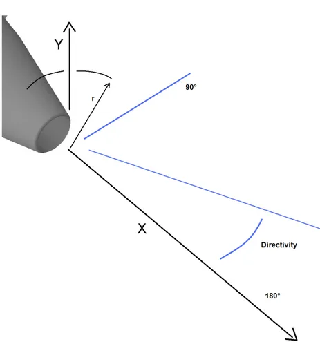
Jet Characterization
Hot‐wire and Pitot tube measurements are performed to verify the jet flow characteristics. The Pitot tube measurements are aimed at verifying the jet symmetry and the characteristics of self‐similarity of the velocity profiles, as well as the axial velocity decrease. The Hot‐wire measurements are performed to obtain high order statistics as axial velocity variance, the skewness and the Kurtosis. The sound measurements in the far‐field complete the jet characterization and allow us to compare the sound spectra with literature data. Figure 36 defines the used reference system for the measurements with the X correspondent with the jet axis.