Monetary Policy and Potential Output Uncertainty:
A QuantitativeAssessment
Simona Delle Chiaie
CEIS Tor Vergata - Research Paper Series, Vol.
32, No. 94, March 2007
This paper can be downloaded without charge from the Social Science Research Network Electronic Paper Collection:
http://papers.ssrn.com/paper.taf?abstract_id=962664
CEIS Tor Vergata
R
ESEARCH
P
APER
S
ERIES
Monetary Policy and Potential Output
Uncertainty: A Quantitative Assessment
Simona Delle Chiaie
yUniversity of Rome, Tor Vergata
January 2007
Abstract
This paper contributes to the recent literature that studies the quantitative implications of the imperfect information about poten-tial output for the conduct of monetary policy. By means of Bayesian techniques, a small New Keynesian model is estimated taking explic-itly account of the imperfect information problem. The estimation of the structural parameters and of the monetary authorities’ objec-tives is key in assessing the quantitative relevance of the imperfect information problem and in evaluating the robustness of previous ex-ercises based on calibration. Finally, the model allows us to analyse the usefulness of unit labor costs as monetary policy indicator.
I am specially grateful to Francesco Lippi for his patient and precious supervising activity. I also thank Fabio Canova, Stefano Neri, Antonio Guarino and seminar partici-pants at the XV International Tor Vergata Conference on Money and Banking for helpful suggestions. Of course I take full responsibility for any errors or omissions. Part of this work was done while the author was visiting the University of Pompeu Fabra, whose kind hospitality is gratefully acknowledged.
yDepartment of Economics, University of Rome ’Tor Vergata’, via Columbia 2, Rome,
1
Introduction
In recent years, central banks’ inability to observe the potential output in real-time has received attention as having important implications for the conduct of monetary policy. For example, Orphanides (2000, 2001), Lansing (2000), Cukierman and Lippi (2005) have highlighted how the signi…cant misperception of potential output, following the productivity slowdown of the early 1970s, may have contributed to the rise of U.S. in‡ation.
Ehrmann and Smets (2003, ES henceforth) provide a description of the economic mechanisms by which the misperception of potential output would have a¤ected in‡ation. Since the central bank has imperfect information about potential output, it cannot discern to what extent ‡uctuations in out-put and in‡ation are due to the di¤erent structural shocks. For instance, following a negative potential output shock, the central bank only observes a fall in output and a rise in price but it cannot perfectly distinguish if these e¤ects are caused by a negative potential output or a positive cost-push shock (or a combination of both). As a consequence of this "information problem", ES argue that, in response to a negative potential output shock, the central bank is forced to assign some probability to the fact that this could be a positive cost-push shock. Hence, even if the central bank uses the best fore-casting procedure, it over-estimates the potential output and under-estimates the output gap. Since, in real-time, the output gap is perceived as negative (while it is actually positive) the central bank will lower the interest rate. In particular, monetary policy will result too loose in comparison to a full information benchmark and this will lead to a higher in‡ation.
model for the euro area. Even though they contribute to clarify in which way potential output uncertainty may a¤ect monetary policy and welfare, however, their quantitative …ndings are driven by the particular set of cali-brated parameter values. For instance, the crucial result of the persistence of output gap forecast errors is clearly a function of the relative variance of po-tential output and cost-push shocks. Common welfare measures, such as the central bank expected losses and its ability to control in‡ation, the output gap and the interest rate adjustments also depend on the covariance matrix of the shocks as well as weights attached to the central bank’s objective func-tion. For these reasons, this paper presents an estimation of the structural parameters and of the monetary authorities’ objectives which is crucial in appraising the quantitative importance of the potential output uncertainty and thus, in evaluating the robustness of these previous calibrations.
By means of Bayesian techniques, this paper estimates a new keynesian dynamic stochastic general equilibrium (DSGE) model which explicitly ac-counts for the imperfect information about the state of the economy. Once the model is estimated, the structural estimates allows us to revisit the issue discussed, among others, by Cukierman and Lippi (2005) and Ehrmann and Smets (2003).
This paper reveals that the quantitative implications of the potential output uncertainty substantially change if di¤erent assumptions on the in-formation set available to the agents are made. In particular, we compare the case in which agents in the economy only use the detrended GDP to infering the output gap level with the alternative situation in which also the real unit labor costs are included into the vector of observables.
Following a potential output shock, the central bank makes a large and persistent error (about 40 quarters) in forecasting the output gap. This error leads optimal monetary policy to deviate from its benchmark value of full information causing an e¤ect on in‡ation which is completely absent in the case of complete information. On the contrary, when the central bank also observes the real unit labor cost to estimating the output gap, the forecast error is quantitatively negligible. As a consequence, the optimal policy does not deviate from its benchmark of full information as well as the in‡ation dynamics are no longer a¤ected by the potential output uncertainty.
Finally, this paper shows that the real unit labor cost plays an important role for monetary policy. Since such indicator provides information about potential output, it strongly improves the central bank’s ability in controlling the output gap target.
The paper proceeds as follows. Next section reviews the model. Sec-tion 3 presents the estimaSec-tion details and comments the results. SecSec-tion 4 analyses the quantitative e¤ects of potential output uncertainty on monetary policy and the role of unit labor cost as monetary policy indicator. Section 5 concludes.
2
The model economy
The model, taken from ES, consists of the following equations: (1) yt= yt 1+ (1 )Etyt+1+ (it Et t+1) + uy;t;
(3) yt= yt 1+ uy;t:
where t; yt; yt; and it denote, respectively, in‡ation, output, potential
output and the nominal short term interest rate. The preference shock uy;t,
the cost - push shock u ;t and the potential output shock uy;t are i.i.d.
inno-vations with zero mean and covariance matrix 2 u:
Since in this speci…cation the dynamics of output and in‡ation depend on both lagged and expected future values, the model is considered as an hybrid version of more traditional backward looking models such as in Svensson (1997a, 1997b) and purely forward looking models such as in Rotemberg and Woodford (1997) and Woodford (1999). As a matter of fact, the hybrid approach arises mostly for empirical reason; in fact while the new generation of Keynesian models may be theoretically more appealing because based on much stronger microfoundations, they cannot explain the persistence existing in the data. In order to account for these features, the presence of the lagged term in the aggregate demand equation has been explicitly motivated by introducing an external habit variable in the household’s utility function while, the lagged in‡ation in the aggregate supply curve has been justi…ed by assuming, in model with staggered prices and wages, partial indexation to past in‡ation rates of prices that cannot be freely set (see e.g. Christiano et al., 2005; Smets and Wouters, 2003).
The model is closed by assuming that the central bank chooses a path for the short-term interest rate minimizing the intertemporal loss function (4) which is over three policy goals: in‡ation, output gap and the change in the short term nominal interest rate.
(4) Et 1 X =0 2 t+ + (yt yt)2+ (it+ it+ 1)2 :
The relative weights and synthesize the preferences of the policymaker over the related policy targets.
It is assumed that the policymaker observes contemporaneous but noisy measures of output, in‡ation and real unit labor cost which are represented by the following vector of measurables:
(5a) yt = yt+ vy;t;
(5b) t = t+ v ;t;
(5c) ct = ct+ vc;t:
The measurement errors in the vector v are assumed to be i.i.d. with covariance matrix 2
v and they are uncorrelated with the vector of innovations
u.
According to the New Keynesian paradigm, the …rms’inability to adjust prices optimally every period creates the existence of a wedge between output and its natural level (output gap). As shown, among others, by Rotemberg and Woodford (1997), the output gap is proportional to deviations of real marginal cost from steady state. Hence, a measure of real marginal cost can be used to approximate (up to a scalar factor) the true, or model-based, output gap. In line with these results, it is …nally assumed that:
(6) ct= (yt yt):
Agents and policymaker in the economy have symmetric information both
on the model parameters, [ ; ; ; ; ; ; ; ; ; 2
u; 2v]and on the whole
history of the observables, therefore the information set It at period t is
represented by It fZ ; t; g :
For estimation purposes it is necessary solving the model. Restricting the attention on the case in which central bank operates in absence of commit-ment, following Svensson and Woodford (2003), the equilibrium (i.e. Markov perfect) under discretion is characterized by the optimal policy rule being a linear function of the current estimate of the predetermined variables. The equilibrium law of motion of the state, forward-looking and indicator vari-ables as well as the optimal predictor of the state vector, are given by:
(7a) it= F Xtjt;
(7b) Xt+1= HXt+ J Xtjt+ Cuut+1;
(7c) Zt = LXt+ M Xtjt+ vt;
(7d) xt= GXtjt+ G1(Xt Xtjt);
(7e) Xtjt= Xtjt 1+ K[L(Xt Xtjt 1) + vt]:
The matrices F; G; G1; H; J; K; L and M are de…ned in Svensson and
Woodford (2003) and depend on the parameters in , whereas Xt0 [ yt 1 t 1 yt uy;t u ;t it 1 ]; x
0
t [ yt t ]; u
0
t [u ;t uy;t uy;t] and Zt0 [yt t
ct ] stand for, respectively, the predetermined state variables, the
forward-looking variables, the structural shocks, the observables and, …nally, it is the
As in recent papers by Schorfheide (1999), Smets and Wouters (2003) and Fernández-Villaverde and Rubio-Ramírez (2004), the model is estimated using Bayesian methods which have been built around the likelihood function derived from DSGE models. Next section presents the estimation details and comments the results.
3
Bayesian analysis
In a Bayesian framework, the sample information represented by the like-lihood function is combined with a priori informations that we may have about model and parameters. Adding a proper prior may down-weight re-gions of the parameter space that are at odds with out-of-sample information and, in which, the structural model becomes uninterpretable. Moreover, even a weakly informative prior may add curvature to a likelihood function that is nearly ‡at in some dimensions of the parameter space clearly facilitating numerical maximization procedures (An and Schorfheide, 2005)1.
3.1
Estimation methodology
The Bayesian analysis requires to transform the solution of the model into a state space form. So, jointly to the equilibrium law of motion of the state, we de…ne a measurement equation that relates the elements of the states vector
1A well known result in Bayesian econometrics (i.e. Poirier, 1998) is that the prior
distribution is not updated in directions of the parameters space in which the likelihood function is ‡at.
to the following set of observables: ft0 [Zt0 it](see equation 13 in appendix).
The vector ftcollects the four series of observations used in this analysis:
output, in‡ation, real unit labor cost and short-term nominal interest rate. Output is measured by the log of seasonally-adjusted real gross domestic product in chained 2000 dollars, the in‡ation rate is provided by the log of the quaterly changes in the seasonally adjusted GDP implicit price de‡ator, real unit labor cost is represented by the series of the log of labor income share in the non-farm business sector and …nally, the three-month U.S. Trea-sury bill rate provides the measure of the nominal interest rate (expressed in percentages per quarter). The data are quaterly, run from from 1947:1 through 2005:4 and they are linearly detrended before the estimation.
It is worthwhile to note that while only two shocks are present in the mea-surement equation (13), the covariance matrix of the endogenous variables is singular. Despite it is not essential for applying the Bayesian techniques however we append an additional measurement error on the interest rate inasmuch it is helpful in computationally reducing the singularity problem.
The Kalman …lter is then applied to the state space system in order to obtain the prediction error decomposition of the likelihood (see, appendix for the analytical derivation). The latter is then combined with a prior distrib-utions of the model parameters to form the posterior density function. Since the analytical solution of the posterior is impossible, Monte-Carlo Markov-Chain (MCMC) sampling methods are used. In particular, a random walk version of the Metropolis Hasting algorithm with small uniform errors is used to generate a Markov chain with stationary distribution that correspond to
the posterior distribution of interest2. It is important to stress that the choice
of the joint prior distribution of the model parameters in‡uences the poste-rior shape hence, it is important to know what features of the posteposte-rior are generated by the prior rather than the likelihood. A direct comparison of priors and posteriors can often provide valuable insights about the extent to which data provide information about the parameters of interest. For these reasons, in the following sections, we discuss the choice of prior distribu-tions, we compare relevant moments of prior and posterior distributions and …nally, we check the robustness of posterior estimates to changes in the prior distributions.
3.2
Priors
Table 1 presents prior distributions of the model parameters. For conve-nience, it is typically assumed that all parameters are a priori independent. Prior distributions are centered around standard calibrated values of the pa-rameters used in the literature while standard errors are chosen in order to cover the range of existing estimates and to avoid to put too much structure on the data. Since priors are loose, the exact form of the densities is chosen
for computation convenience. For the parameters ; ; and which must
lie in the interval [0,1) Beta distributions are chosen. All the variances of shocks are assumed to be distributed as a Gamma distribution because it assures a positive variance with a rather large domain. Gamma distribution
2Variance of errors is set in order to obtain an acceptance rate of about 35-40%. The
is also used for the in‡ation elasticity to the output gap in order to in-clude in its domain the wide range of estimated and calibrated parameter values suggested by the literature. Finally, normal distribution is chosen for remaining parameters.
Table 1 - Prior distributions
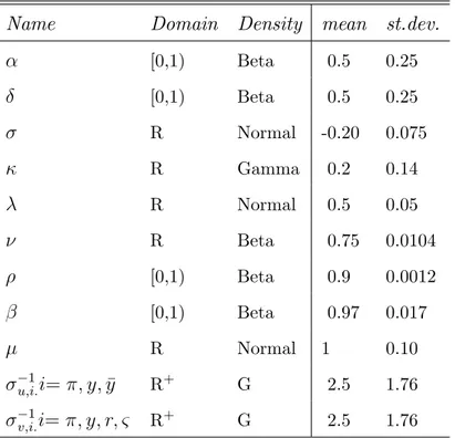
Name Domain Density mean st.dev.
[0,1) Beta 0.5 0.25 [0,1) Beta 0.5 0.25 R Normal -0.20 0.075 R Gamma 0.2 0.14 R Normal 0.5 0.05 R Beta 0.75 0.0104 [0,1) Beta 0.9 0.0012 [0,1) Beta 0.97 0.017 R Normal 1 0.10 1 u;i:i= ; y; y R+ G 2.5 1.76 1 v;i:i= ; y; r; & R+ G 2.5 1.76
3.3
Findings
The Bayesian analysis produces reasonable posterior distributions for the model parameters. Except for the discount factor , data are informative in the sense that posterior distributions of the model parameters are more con-centrated and rather shifted relative to the priors. Table 2 presents relevant statistics of the posterior distributions of the model parameters. Focusing
on the posterior distribution of the backward-looking component of the New-Keynesian Phillips curve, one observes that, in spite of a relatively loose prior on this parameter, the posterior distribution has a small dispersion with a range that goes from 0.38 to 0.41. These …ndings imply a degree of in‡ation inertia greater than in Gali and Gertler (1999), Gali, Gertler and Lopez-Salido (2001), supporting the view that both backward looking and forward looking behaviors are important in shaping the U.S. in‡ation dynamics. The posterior distribution of the Phillips curve slope suggests a signi…cant e¤ect of real activity on in‡ation. The posterior mean is 0.07 and it is close to the estimates of obtained by Gali and Gertler (1999) and Gali, Gertler and Lopez - Salido (2005) using GMM3.
Regarding the structural parameters of the aggregate demand equation, the estimation suggests that both backward and forward looking components are signi…cant in explaining output dynamic. The posterior mean of the elasticity of output to the real interest rate is -0.30 and it is quite consistent with other previous results found in the Real Business Cycle literature. The analysis also delivers plausible estimates for the parameters describing the preferences of the monetary authority. The posterior mean of the weight attached to the output gap is 0.47 suggesting that the policymaker looks out for the deviation of output from its natural level. The estimates of
3In a …rst version of this paper, the model was estimated by excluding the unit labor cost
indicator. The estimation results showed that the Phillips curve slope estimate was close to zero and moreover, the standard deviations of the cost-push shock and the measurement errors were very high. These …ndings suggested to re-estimate the model taking into account a better proxy for the output gap rather than the detrended GDP (i.e. Gali and Gertler (1999)).
(0.58) provides evidence of a substantial degree of interest rate smoothing. Anyway, the posterior distribution of is bimodal so that care should be exercised in using the posterior mean as a measure of location. The estimates of the structural shocks ( u) show that cost-push and potential output shocks
have the largest standard deviation.
Table 2 - Posterior distributions Name Relevant statistics
mean median st.d. min max
0.4059 0.4126 0.0105 0.382 0.414 0.7171 0.6833 0.0593 0.656 0.904 -0.2957 -0.2933 0.0051 -0.314 -0.282 0.0712 0.0167 0.1417 0.0002 0.608 0.4689 0.4653 0.0084 0.456 0.501 0.5764 0.5699 0.0167 0.554 0.632 0.9291 0.9763 0.0782 0.757 0.999 1.606 1.6977 0.1722 1.083 1.773 0.9411 0.9473 0.0644 0.459 0.999 u;y 1.4271 1.7334 0.4952 0.126 1.752 u;y 0.3555 0.4169 0.0985 0.099 0.419 u; 1.472 1.7464 0.4543 0.1 1.758 v;y: 0.1619 0.1830 0.0401 0.031 0.189 v; 0.2731 0.2735 0.0595 0.017 0.373 v;r 1.4323 1.6702 0.0039 0.048 1.706 v;& 0.0592 0.0609 0.4272 0.045 0.067
Table 3 - Asymptotic variance decomposition
Fundamental shocks Measurement errors
pot dem cos out in‡ ulc
Output 59.09 11.03 29.48 0.04 0.35 0.01
Output gap 59.03 11.02 29.46 0.05 0.43 0.02
In‡ation 1.26 0.35 98.28 0 0.10 0
Interest changes 37.23 19.05 40.66 1.40 1.65 0.02
The variance decomposition of Table 3 indicates that cost-push shocks are the main source of ‡uctuations for in‡ation and they also explain a large part of the interest rate volatility. Demand shocks explain a substantial part of the variance of output and interest rate. Finally, potential output shocks explain more than one half of the output gap volatility. The estimates also show that the measurement error concerning real unit labor cost is rather small. Instead, the measurement errors of output and in‡ation are signi…-cant (0.16 and 0.27, respectively), even if the variance decomposition analysis of Table 3 indicates that they have a marginal role in explaining the vari-ables’‡uctuations. Figure 1 describes the model …t by plotting the one-step ahead predictions for each of the four variables used in estimation. The …gure shows that the model forecasting performance is rather accurate for nominal variables. The correlation between the one-step-ahead prediction and actual values is 0.78 and 0.76 for in‡ation and nominal interest rate respectively, indicating that the model is able in predicting high frequency in‡ation move-ments. The model forecasting performance is more modest with respect to
output (0.58) and real unit labor cost (0.59). 1947 1959 1971 1984 1996 2008 -0.04 -0.02 0 0.02 0.04 0.06 output 1947 1959 1971 1984 1996 2008 -0,02 -0.01 0 0,01 0,02 0,03 0,04 inflation 1947 1959 1971 1984 1996 2008 -0.01 0 0.01 0.02 0.03 0.04
short term nominal interest rate
1947 1959 1971 1984 1996 2008 -0.02 -0.01 0 0.01 0.02 0.03 0.04 0.05
real unit labor costs
fitted real corr coef 0.5735 corr coef 0.7661 corr coef 0.7590 corr coef 0.5840
Figure 1 - Data (dotted line) and one-step ahead forecasts (solid line)
Finally, we analyse the robustness of posterior estimates to changes in the prior distribution. Table 4 reports the posterior moments of the prior and the posterior in the baseline case and the posterior moments in two alternative speci…cations, obtained making the prior progressively more informative. In particular, we mantain the same measures of location but the probabilities
density are rescaled by reducing the prior ranges by 10 and 20 percents. Table 4 - Robustness analysis
name posterior (90% spread) posterior (80% spread)
mean median sd mean median sd
0.4593 0.4683 0.0142 0.4593 0.4683 0.0142 0.7156 0.7234 0.0250 0.7156 0.7234 0.0250 -0.2109 -0.2124 0.0031 -0.1279 -0.1313 0.0073 0.0672 0.0125 0.1365 0.063 0.0086 0.1304 0.4965 0.4885 0.0181 0.5226 0.5077 0.0332 0.5607 0.5506 0.0257 0.5158 0.4935 0.0563 0.9287 0.9311 0.0685 0.9599 0.9222 0.0306 1.1186 1.0063 0.2528 1.0562 1.0000 0.1928 0.8909 0.8366 0.2040 0.8539 0.8286 0.4121 u;y 1.3137 1.5714 0.4274 1.1773 1.3789 0.3497 u;y 0.3722 0.4412 0.1118 0.3917 0.4698 0.1273 u; 1.3537 1.5811 0.3863 1.2115 1.3852 0.3087 v;y: 0.1514 0.1770 0.0482 0.1405 0.1685 0.0511 v; 0.2828 0.2842 0.0697 0.2945 0.2958 0.0779 v;r 1.3234 1.5237 0.3699 1.1912 1.3476 0.3039 v;& 0.0267 0.0284 0.0038 0.0099 0.0109 0.0022
Following, Geweke (1998), posterior draws from the new distribution are obtained reweigthing the posterior draws obtained in the baseline case with w( ) = ggBi( )( ) where the g
i( ) is the new prior and gB( ) is the baseline one.
in the prior speci…cation.
4
Potential Output Uncertainty and
Mone-tary Policy
In this section the estimated model is used to analyse the quantitative e¤ects of the imperfect information about potential output and also to assess the usefulness of unit labor cost as monetary policy indicator. Throughout this section, we compare outcomes of two di¤erent situations. The …rst situation is one with complete information (CI) which implies that all agents in the economy perfectly observe current output, in‡ation, real unit labor cost and nominal interest rate as well as current potential output. In the second more realistic situation, the central bank and the private sector are subject to incomplete information (II) about potential output. This implies that agents do not observe potential output directly and moreover, it is supposed that they only have noisy indicators. From the demand equation, it is clear that the central bank and the private sector will be able to estimate the demand shock perfectly, whereas they will face a signal extraction problem in trying to distinguish cost-push shocks from potential output shocks. This problem may create a misperception of the potential output even though we present how di¤erent scenarios may emerge if the real unit labor cost indicator is available to the agents or not.
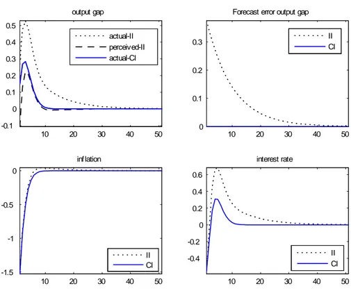
Figure 2 presents the responses of output, in‡ation, actual and perceived output gap, nominal interest rate and the output gap forecast error following a positive shock to potential output when the real unit labor cost indicator
is removed from the central bank’s vector of observables. 10 20 30 40 50 -0.8 -0.6 -0.4 -0.2 0 output gap 10 20 30 40 50 -0.8 -0.6 -0.4 -0.2 0
Forecast error output gap
10 20 30 40 50 -0.15 -0.1 -0.05 0 inflation 10 20 30 40 50 0 0.2 0.4 0.6 0.8 1 interest rate actual-II perceived-II actual-CI II CI II CI II CI
Figure 2 - Complete vs Incomplete information (positive potential output shock)
One may observe that the central bank makes a large and persistent error in forecasting the output gap. The reasons for such an error hinge on the above signal extraction problem. Following a positive potential output shock, the central bank just observes a rise in output and a fall in price but it does not perfectly recognize if those e¤ects are caused by a positive potential output or a negative cost-push shock (or a combination of both). As a result,
it assigns some probability to the fact that this is actually a negative cost-push shock in this way causing an under-prediction of the potential output. The upper part of the …gure shows that for about 40 quarters the cen-tral bank perceives a positive output gap while it is actually negative. The output gap forecast error leads the optimal interest rate to deviate from the benchmark value under perfect information causing a larger fall in the output gap and a larger fall in in‡ation.
10 20 30 40 50 -0.1 0 0.1 0.2 0.3 0.4 0.5 output gap actual-II perceived-II actual-CI 10 20 30 40 50 0 0.1 0.2 0.3
Forecast error output gap
II CI 10 20 30 40 50 -1.5 -1 -0.5 0 inf lation II CI 10 20 30 40 50 -0.4 -0.2 0 0.2 0.4 0.6 interest rate II CI
The opposite occurs in response to a negative cost-push shock. In this case the central bank assigns some probability that this is actually a positive potential output shock under-predicting the output gap. As a result, it will lower the interest rate by more than it would otherwise have done. This leads to a larger response in the output gap, and a smaller fall in in‡ation.
Figure 4 compares the responses of the variables of interest following a positive potential output when the central bank can infer the level of potential output based on output and real unit labor cost, too.
10 20 30 40 50 -0.6 -0.5 -0.4 -0.3 -0.2 -0.1 0 output gap actual-II perceived-II actual-CI 10 20 30 40 50 -6 -5 -4 -3 -2 -1 0
x 10-4 Forecast error output gap
II CI 10 20 30 40 50 -0.12 -0.1 -0.08 -0.06 -0.04 -0.02 0 inflation II CI 10 20 30 40 50 0 0.2 0.4 0.6 0.8 1 interest rate II CI
Figure 4 - E¤ects of a positive potential output shock (agents observe real unit labor cost)
It is important to note that, in this case, the error in forecasting the output gap is quantitatively negligible. As a result, the certainty equivalent policy rule tracks the one we would expect if information was perfect and the in‡ation dynamics are not a¤ected by the potential output uncertainty.
Figure 5 con…rms the above conclusions for the case of a negative cost-push shocks: The forecast error is tiny and the dynamics of all variables of interest completely overlap their benchmarks of full information.
10 20 30 40 50 0.05 0.1 0.15 0.2 0.25 output gap actual-II perceived-II actual-CI 10 20 30 40 50 0 1 2 3 4
x 10 -5 Forecast error output gap
II CI 10 20 30 40 50 -1.4 -1.2 -1 -0.8 -0.6 -0.4 -0.2 inflation II CI 10 20 30 40 50 -0.4 -0.2 0 0.2 interest rate II CI
Figure 5 - E¤ects of a negative cost-push shock (agents observe real unit labor cost)
The …nding that the forecast error is very small when real unit labor cost is employed in estimating the output gap suggests that such indicator contains useful information on potential output. At the same time, this result con…rms the objection raised by Gali and Gertler (1999), Gali and Gertler and Lopez-Salido (2001, 2005) in using the detrended GDP (the deviations of log GDP from a smooth trend) as a proxy for the output gap in empirical applications. 1947 1952 1957 1962 1967 1972 1977 1982 1987 1992 1997 2002 2007 -0.04 -0.03 -0.02 -0.01 0 0.01 0.02 0.03 0.04
Potential output estimates and current inflation
time
estimated potential output inflation
estimated potential output (no ulc)
Figure 6 - Potential output estimates and current in‡ation
Figure 6 presents an informal assessment of this point based on the pat-terns of cross-correlations between two alternative estimates of potential
out-put and in‡ation. The violet line corresponds to the potential outout-put esti-mate obtained using both output and real unit labor cost indicators. The green line corresponds to the counterfactual estimate obtained by removing the unit labor cost indicator from the central bank’s vector of observables. This visual experiment shows that when the output gap indicator is not avail-able, the estimated potential output is a smooth series and it is clear that no obvious correlation among this estimate of potential output and the in‡ation rate (blu line) exists.
Table 5 - Welfare e¤ects of observing unit labor cost Indicators
in‡ation, output, unit labor costs no unit labor costs
output gap 1.38 3.52
in‡ation 2.74 2.81
interest changes 1.73 1.69
expected losses 238.75 369.29
Finally, we study the usefulness of unit labor cost indicator throught the e¤ects it produces on some welfare measures. Once again, we analyse how economic performance is a¤ected by the removal of such indicator from the vector of observables. Table 5 reports the standard deviation of target variables (output gap, in‡ation and interest rate changes) and central bank expected losses. The …rst column considers the case in which all indicators are available to the central bank. The second one instead shows the values
of these variables in the case in which unit labor costs are taken away from the central bank’s information set.
This exercise shows that expected losses signi…cantly increase when that indicator is removed from the vector of observables. This e¤ect is mainly due to the raise of the standard deviation of the output gap and in‡ation. On the contrary, the volatility of the interest rate changes has a little decline. This last result means that when unit labor costs are taken away from the information set, the greater uncertainty concerning the estimate of potential output causes a reduction in monetary policy activism.
5
Conclusions
This paper contributes to the recent literature that studies the quantita-tive implications of the imperfect information about potential output for the conduct of monetary policy. For this purpose, a small New Keynesian model which explicitly accounts for the imperfect information problem, is estimated by means of Bayesian techniques.
The Bayesian analysis produces reasonable posterior distributions for the model parameters. In particular, the posterior distribution of the Phillips curve slope suggests a signi…cant e¤ect of real activity on in‡ation and it is consistent with those of Gali and Gertler (1999), Sbordone (1999), Gali, Gertler and Lopez-Salido (2005).
Using the estimates of the structural parameters and of the monetary authority’s objectives, this paper analyses the quantitative relevance of the imperfect information about potential output for monetary policy.
When the information set available to the agents only includes noisy mea-sures of output and in‡ation, this work corroborates the Ehrmann and Smets (2003) conclusion that following a potential output shock, the central bank makes a large and persistent error in forecasting the output gap. This error leads the optimal policy to deviate from the benchmark value of full informa-tion creating an e¤ect on in‡ainforma-tion which is completely absent in the case of perfect information. On the contrary, we show that when the real unit labor cost indicator is available to the agents, following a shock to potential output, the output gap forecast error is quantitatively negligible. As a consequence, the optimal policy does not deviate from its benchmark of full information as well as the in‡ation dynamics are not a¤ected by the potential output uncertainty.
Finally, this paper shows the relevance of the real unit labor cost as monetary policy indicator. Our …ndings suggest that real unit labor cost contains information on potential output and this, in turn, improves the central bank’s ability in making stabilization policy more e¤ective.
Appendix
Using (7e) and (7b) I get
(8) Xt+1= (H + J KL)Xt+ J (I KL)Xtjt 1+ J Kvt+ Cuut+1;
taking expectations and using (7e) we obtain
(9) Xt+1jt = (H + J )(I KL)Xtjt 1+ (H + J )KLXt+ (H + J )Kvt:
we can rewrite (8) and (9) as follows
(10) St+1 = ASt+ Be1;t+1; by de…ning St+1 Xt+1 Xt+1jt A = 2 4 (H + J KL) J (I KL) (H + J )KL (H + J )(I KL) 3 5 ; B = 2 4 Cu J K 0 (H + J )K 3 5 and e1;t+1= 2 4 ut+1 vt 3 5
In the same way, substituting (7e) into (7a) and (7c) we get
(12) it = (F F KL)Xtjt 1+ F KLXt+ F Kvt:
Finally, we can rewrite (11) and (12) in state-space form:
(13) ft= CSt+ Dvt; where ft0 [Zt0it]; C = 2 4 L + M KL M (I KL) F KL F (I KL) 3 5 ; D = 2 4 I + M K F K 3 5 .
adding a vector of measurement errors we get
(14) ft= CSt+ e2;t;
where e2;t Dvt + t: is the vector of measurement errors and t
h 0 0 i;t i0 : (15) V1 E(e1;t+1e 0 1;t+1) = 2 4 2 u 0 0 2 v 3 5 ; (16) V2 E(e2;te 0 2;t) = D 2vD 0 + E( t 0t); (17) V3 E(e1;t+1e 0 2;t) = 2 4 0 2 vD0 3 5 :
The Kalman …lter is then applied to the state space model (10) and (14). That …lter takes the observations of ftfor t = 1; 2; :::::T and works recursively
(18) wt= ft ftjt 1 = ft CStjt 1;
where ftjt 1 is the prediction of the observable variables given the infor-mation available at period t and the forecast error covariance matrix is given by: (19) t E(wtw 0 t) = E(ft ftjt 1)(ft ftjt 1) 0 = = E[(CSt+ e2;t CStjt 1)(CSt+ e2;t CStjt 1) 0 ] = = Ef[C(St Stjt 1) + e2;t][C(St Stjt 1) + e2;t]g 0 = = E[C((St Stjt 1)(St Stjt 1) 0 C0] + E(e2;te 0 2;t) = C 2tjt 1C 0 + V2: where 2 tjt 1 = E(St Stjt 1)(St Stjt 1) 0 :
Since by construction, the forecast error wt is serially uncorrelated and
normally distributed for all t = 1; 2; ::::; T:with mean zero and covariance matrix t;then log-likelihood function is given by:
(20) ln L = nT 2 log(2 ) 1 2 T X t=1 lnj tj 1 2 T X t=1 wt t1w 0 t:
The optimal predictor of the states vector using the Kalman …lter is given by: (21) St+1jt = AStjt 1+ Ktwt; where (22) Kt (A 2tjt 1C 0 + BV3)(C 2tjt 1C 0 + V2) 1; (23) 2t+1jt = (A 2tjt 1A0 + BV1B 0 ) Kt(A 2tjt 1C 0 + BV3) 0 :
where the matrix Ktis the Kalman gain and 2t+1jt E(St+1 St+1jt)(St+1
References
[1] An, S. and F. Schorfheide (2005). "Bayesian analysis of DSGE models", forthcoming, Econometric Reviews.
[2] Brainard, C. (1967). "Uncertainty and the E¤ectiveness of Policy", The American Economic Review 57 (2), 411-425.
[3] Canova, F. (2006). "Methods for applied macroeconomic research", forthcoming, Princeton University Press.
[4] Clarida, R., Galí, J. and M. Gertler (1999). "The science of monetary policy: A New-Keynesian Perspective”, Journal of Economic Literature 37, 1661-1707.
[5] Christiano, L., Eichenbaum M. and C. L. Evans (2005). “Nominal rigidi-ties and the dynamic e¤ects of a shock to monetary policy”, Journal of Political Economy 113 (1), 1-45.
[6] Cukierman, A. and F. Lippi (2005). "Endogenous monetary policy with unobserved potential output”, Journal of Economic Dynamics and Con-trol,
[7] Ehrmann, M. and F. Smets (2003). "Uncertain potential output: im-plications for monetary policy”, Journal of Economic Dynamics and Control 27, 1611-1638.
[8] Fernandez-Villaverde, J. and J. Rubio-Ramirez (2001). ”Comparing Dy-namic Equilibrium Models to the data, University of Pennsylvania, man-uscript.
[9] Galí, J., Gertler M. and D. López-Salido (2001). “European In‡ation Dynamics", European Economic Review 45 (7), 1237-1270.
[10] Galí, J., Gertler M. and D. López-Salido (2005). "Robustness of the esti-mates of the hybrid New Keynesian Phillips curve". Journal of Monetary Economics 52, 1107-1118.
[11] Galí, J. and M. Gertler (1999). "In‡ation Dynamics: A Structural Econometric Analysis,”Journal of Monetary Economics 44 (2), 195-222. [12] Gerali A. and F. Lippi (2003). “Optimal Control and Filtering in Linear Forward-Looking Economies: A Toolkit”, CEPR Discussion Papers, No. 3706.
[13] Ireland, P.N. (2004). "A method for taking models to the data”, Journal of Economic Dynamics and Control 28, 1205-1226.
[14] Lansing, K. (2000). "Learning about a shift in trend output: implica-tions for monetary policy and in‡ation", Federal Reserve Bank of San Francisco Working Paper 2000-16.
[15] Lindé, J. (2002). “Estimating New-Keynesian Phillips Curves: A Full Information Maximum Likelihood Approach”, Sveriges Riksbank Work-ing Paper Series No. 129.
[16] Lippi, F. and S. Neri (2005). ”Information variables for monetary policy in an estimated structural model of the euro area”, NBER Working Paper.
[17] Orphanides, A. (2000). ”The quest for prosperity without in‡ation”, ECB Working Paper, 15.
[18] Otrok, C. (2001). "On measuring the welfare cost of business cycles", Journal of Monetary Economics 47, 61-92.
[19] Orphanides, A. (2001). "Monetary policy rules based on real-time data”, American Economic Review 91 (4), 964-985.
[20] Rotemberg, J. and M. Woodford (1997). "An Optimization-Based Econometric Framework for the Evaluation of Monetary Policy" in Ben Bernanke and Julio Rotemberg (eds.) NBER Macroeconomics Annual 1997, MIT Press, Cambridge, MA.
[21] Sbordone, A.M. (1998). Prices and Unit Labor Costs: Testing Models of Pricing. Princeton University, mimeo.
[22] Schorfneide, F. (2000). "Loss function-based evaluation of DSGE mod-els", Journal of Applied Econometrics 15, 645-670.
[23] Smets, F. and R. Wouters (2003). “An Estimated Stochastic General Equilibrium Model of the Euro Area”, Journal of the European Eco-nomic Association 1, 1123-1175.
[24] Svensson, L.E.O. (1997a). "In‡ation Forecast Targeting: Implement-ing and MonitorImplement-ing In‡ation Targets", European Economic Review 41, 1111-1147.
[25] Svensson, L.E.O. (1997b). "In‡ation Targeting: Some Extentions", NBER Working Paper Series 5962.
[26] Svensson, L.E.O. and M. Woodford (2003). ”Indicator variables for op-timal policy”, Journal of Monetary Economics 50, 691-720.
[27] Woodford, M. (1999). "Optimal monetary policy inertia", NBER Work-ing Paper Series 7261.