1D Atmosphere Models from Inversion of Fe I 630 nm Observations with an Application to Solar Irradiance Studies

2021-02-16T16:30:35Z

Acceptance in OA@INAF

1D Atmosphere Models from Inversion of Fe I 630 nm Observations with an

Application to Solar Irradiance Studies

Title

Cristaldi, A.; ERMOLLI, Ilaria

Authors

10.3847/1538-4357/aa713c

DOI

http://hdl.handle.net/20.500.12386/30415

Handle

THE ASTROPHYSICAL JOURNAL

Journal

841

revealed by high-resolution solar observations. We aimed to derive observation-based atmospheres from such observations and test their accuracy for SI estimates. We analyzed spectropolarimetric data of the FeI630 nm line pair in photospheric regions that arerepresentative of the granularquiet-Sun pattern (QS) and of small- and large-scale magnetic features, both bright and dark with respect to the QS. The data were taken on 2011 August 6, with the CRisp Imaging Spectropolarimeter at the Swedish Solar Telescope, under excellent seeing conditions. We derived atmosphere models of the observed regions from data inversion with the SIR code. We studied the sensitivity of results to spatial resolution and temporal evolution, and discussthe obtained atmospheres with respect to several 1D models. The atmospheres derived from our study agree well with most of the1D models we compare our results with, both qualitatively and quantitatively (within 10%), exceptfor pore regions. Spectral synthesis computations ofthe atmosphere obtained from the QS observations return anSI between 400 and 2400 nm that agrees, on average, within 2.2% with standard reference measurements, and within−0.14% with the SI computed on the QS atmosphere employed by the most advanced semi-empirical model of SI variations. Key words: Sun: atmosphere– Sun: faculae, plages – Sun: magnetic fields – Sun: photosphere – sunspots

1. Introduction

The solar irradiance(SI) is the fundamental source of energy entering the Earth’s system. Accurate knowledge of its variations is thus crucial to understand the externally driven changes to the system, and, in particular, to the regional and global Earthclimate (see, e.g., Haigh 2007; Solanki et al.

2013). Regular monitoring of the total SI (TSI1) and of the

spectral SI(SSI) in the ultraviolet (UV), carried out since 1978 with satellite measurements, has shown that the SI varies on timescales from tens of seconds to decadesand in all spectral bands. In particular, available measurements show TSI variations of ≈0.1% in phase with the 11-yearsolar cycle, and of up to ≈0.3% on the timescales of solar rotation. It is worth noting thaton the whole, 30%–60% of the TSI variations over the solar cycle are produced at UV wavelengths (Lean et al. 1997; Krivova et al. 2006), whichover the same

periodchange byup to 100% and even more (e.g., Rottman

2006; Fröhlich2013; Kopp2016, and references therein). UV SSI variations can have a significant impact on the Earth’s climate system. Indeed, the SSI below 400 nm takes an active part ingoverning the chemistry and dynamics of the Earth’s upper stratosphere and mesosphereby affecting production, dissociation, and heating processes of ozone, and other components; this also implies changes in winds and atmo-spheric circulation (e.g., Solanki et al. 2013, and references therein).

In order to accurately estimate effects of SI variations on the Earth’s system, climate models require long and precise series of SI data. Owingto theshort duration and difficult calibration

of the available measurements, satellite recordsstill suffer uncertainties, however, e.g., on the TSI trends measured on timescales longer than the 11-yearcycle and on the SSI changes occurring at some spectral bands(Ermolli et al.2013; Solanki et al. 2013). In addition to improvingour

under-standing of the physical processes responsible for the measured SI changes, precise models of SI can also support the analysis of the existing SI records for Earth’s climate studiesby allowing us to interpret, complement, and extend available data series.

Models that ascribe variations in SI ontimescales greater than a day to solar surface magnetism are particularly successful in reproducing existing SI observations (e.g., Domingo et al. 2009). There are two classes of such models,

called proxy and semi-empirical (Ermolli et al. 2013; Yeo et al.2014a,2014b). The former class of SI models combines

proxies of solar surface magnetic features using regressions to match observed TSI changes. The proxies most frequently used are the photometric sunspot index and the chromospheric MgII

index, to describe the sunspot darkening and facular bright-ening, respectively. The semi-empirical SI models reproduce SI variations by summingthe contributions to SI of the different features observed on the solar diskin time. For each time and observed feature, they employ the surface area and position covered by the feature at the given timeand its time-invariant brightness as a function of wavelength and position on the solar disk. The latter quantity is calculated from the spectral synthesis performed under some assumptions on semi-empiri-cal, one-dimensional, plane-parallel, static atmosphere models (hereafter 1D models) representative of the observed feature (see, e.g., Ermolli et al. 2013; Yeo et al. 2014a, 2014b).

Examples of the 1D models employed in SI reconstructions are 1

The spectrally integrated solar radiativeflux incident at the top of Earth’s atmosphere at the mean distance of one astronomical unit.

the ones presented by Vernazza et al. (1981), Fontenla et al.

(1993, 1999, 2009, 2011, 2015), Kurucz (1993, 2005), and

Unruh et al.(1999).

Present-day, most advanced semi-empirical SI models(e.g., SATIRE-S, Yeo et al. 2014b) replicate more than 95% of the

TSI variability measured over cycle 23 and most of the SSI changes detected on rotational timescales, especially between 400 and 1200 nm. Despite the excellent match of modeled to measured SI, current semi-empirical SI models still need improvements to overcome some limitations due to e.g., application of free parameters and of simplifying assumptions. Besides, from computations of the radiative transfer (RT) in atmospheres resulting from magneto-hydrodynamic simula-tions, it was shown that“a one-dimensional atmospheric model that reproduces the mean spectrum of an inhomogeneous atmosphere necessarily does not reflect the average physical properties of that atmosphere and is therefore inherently unreliable” (Uitenbroek & Criscuoli 2011). This casts doubts

on the accuracy of 1D models employed in SI reconstructions, particularly to account for the radiant properties of the small-scale features observed on the solar disk (Uitenbroek & Criscuoli 2011; Criscuoli 2013; Yeo et al.2014a,2014b).

In this paper, we derive atmosphere models of various solar photospheric features from inversion of spectropolarimetric observations, and discuss the results obtained with respect to the 1D models that aremost widely employed in SI reconstructionsand other 1D models derived from spectro-polarimetric data. In the following sections we describe the observations and data analyzed in our study, and the methods applied(Section 2). Then we present the results derived from

the data inversion(Section3) and discuss them with respect to

1D models in the literature(Section4). Finally, we investigate

the accuracy of using the obtained models in SI reconstructions (Section 5), discuss the results obtained from our study, and

draw our conclusions (Section6).

2. Data and Methods 2.1. Observations

The data analyzed in our study were acquired on 2011 August 6, from 07:57 UT to 10:48 UT, with the CRisp Imaging Spectropolarimeter (Scharmer et al.2008) at the Swedish 1 m

Solar Telescope (SST, Scharmer et al. 2003). They consist of

full-Stokes spectropolarimetric measurements derived from a scan of 30wavelengthsof the photospheric FeIdoublet, from 630.12 to 630.28 nm, over afield of view (FOV) of ≈57×57 arcsec2, at three diskpositions. Thespectropolarimetric scans of 30 wavelengthswere taken with a cadence of 28 s and a spectral sampling of »0.0044 nm. The above data are complemented with simultaneous and cospatial chromospheric broadband images taken at the core of the CaII H line at 396.9 nm; in this study, these data were employed to check our identification of the bright magnetic regions described in the following. The observations were assisted by the adaptive optics system of the SST(Scharmer et al.2003)under excellent

seeing conditions.

The pixel scale of the analyzed observations is »0.059 arcsec/pixel. The polarimetric sensitivity of the analyzed data, which was estimated as the standard deviation of the Stokes Q, U, and V profiles in the continuum, is <3.3×10−3 of the continuum intensity for all the Stokes parameters.

The observations targeted a quiet-Sun (QS) region at diskcenter, the active region (AR) NOAA 11267 (AR1) consisting of two sunspots of opposite polarity at diskposition [S17, E24, cosine of the heliocentric angle μ=0.84], and a mature spot in AR NOAA 11263(AR2) at diskposition [N16, W43,μ=0.76]. The data of the three above regions were also analyzed by Stangalini et al.(2015), Cristaldi et al. (2014), and

Falco et al. (2016), respectively. More details about the

analyzed observations can be found in the above papers. The observations were processed with the standard reduction pipeline (CRISPRED, de la Cruz Rodríguez et al. 2015)to

compensatefor the dark and flat-field response of the CCD devices, and for instrument- and telescope-induced polarizations. They were also restored for seeing-induced degradations by using the multi-object multi-frame blind deconvolution technique (MOMFBD, van Noort et al.2005, and references therein).

We analyzed all the data available for the three observed regions, that means series of 79, 101, and 117 sequences of measurements taken over 47, 37, and 56 minutes for the QS, AR1, and AR2 regions, respectively. We extracted subarrays (hereafter referred to as subFOV) of 100×100 pixels represen-tative of QS regions, small-scale bright magnetic regions such as bright points and network(BPs), large-scale, bright regions with strong magneticfield suchas plages (PL), small-scale and large-scale dark magnetic regions suchas pores (PO) and umbrae (UM), respectively. Each analyzed subFOV represents a ≈6×6 arcsec2region on the solar disk. This region is onthe same order as the elementary area considered when identifying bright and dark solar features in full-diskobservations employed in semi-empirical SI models. Indeed, the spatial resolution of theanalyzed data ranges from ;8 to 1 arcsecfor earlier ground-based and more recent space-borne observations.

Figure 1 shows examples of the QS, AR1, and AR2 observations analyzed in our study. For each region, we show the measured continuum intensity and signed circular polariza-tion(CP) maps. The latter quantity has been computedfollow-ing Requerey et al.(2014)as



å

subFOV, V is the Stokes-V profile, and i runs over the 10 spectral points closer to the core of the FeIline at 630.25 nm. In the weak-field regime, the CP can be considered as a proxy for the longitudinal component of the magnetic field (Landi Degl’Innocenti & Landolfi2004).

The red boxes in the various panels of Figure1 show the subFOVs considered in the following to represent the physical properties of QS, BPs, PL, PO, and UM regions. The blue boxes in the middle panels of Figure 1 show two more PL regions that arealso analyzed in our study and discussed in Section5.

2.2. Semi-empirical 1D Atmosphere Models

For the purpose of discussing the results derived from the above observations, we analyzed several sets of 1D models presented in the literature. In particular, we considered the atmosphere model presented by Vernazza et al. (1981) to

represent QS regions (VAL-C), and the sets of models by Fontenla et al. (1993, 1999, 2006, 2011, 2015) to describe

various solar features, from the faint granular cell interior (FAL-A) and average cell (FAL-C) in QSto network (FAL-E), enhanced network (FAL-F), plage (FAL-H), bright plage (FAL-P), penumbral (FAL-R), and umbral (FAL-S) regions. These latter models are employed,e.g., inthe SRPM semi-empirical SI reconstructions (Fontenla et al. 2015, and references therein). Note that the Fontenla et al. (2015) models

are neither discussed nor displayed in the following, since their

difference with respect to previous models by Fontenla et al. (2011) is not appreciable at the scale of the plots and at the

range of atmospheric heights considered in our study. We also analyzed other available 1D models obtained from inversion of spectropolarimetric observations. In particular, we considered the SOLANNT and SOLANPL flux-tube models by Solanki (1986) and Solanki & Brigljevic (1992) for network and plage

regions, respectively, and the COOL and HOT models by

Figure 1.Example of the observations and subFOVs analyzed in our study. Continuum image(left) and circular polarization map (right) of the studied QS (top), active region AR1(middle), and mature spot AR2 (bottom). The red boxes in each panel show the inverted subFOVs, representative of unmagnetized (quiet, QS), bright points(BPs), plage (PL), pore (PO), and umbral (UM) regions, labeled 1, 2, 3, 4, and 5, respectively. Blue boxes in AR1 marktwo more plage regions (labeled 4a and 4b) that arealso analyzed in our study and discussed in Section5.

Collados et al. (1994) for large and small spots, in the order

given; all these models are available in the SIR code described below. Finally, we tested the results derived from our study also with respect to the Harvard-Smithsonian Reference Atmosphere (HSRA, Gingerich et al.1971) and the model by

Maltby et al.(1986) for average QS regions, and the M-model

by Maltby et al.(1986) for spots. Table1 summarizes all the 1D models analyzed in our study.

2.3. Stokes Inversions

We performed full-Stokes spectropolarimetric local thermo-dynamic equilibrium(LTE) inversions of the available data for the selected subFOVs with the SIR code (Stokes inversion based on response functions, Ruiz Cobo & del Toro Iniesta 1992; Bellot Rubio 2003). We applied the code

simultaneously to measurements of the FeI lines at 630.15 and 630.25 nmby excluding from the calculation the Stokes-I measurements in the red wing of the FeI line at 630.25 nm, which are affected by telluric blends. The SIR code uses the atomic parameters taken from the VAL-D database (Piskunov et al. 1995). For each analyzed subFOV, we first normalized

the measurements to the average continuum intensity measured on a nearby QS region, defined as the region with aCP signal lower than threetimes the standard deviation of the entire CP map.

We performed the data inversion by considering(a) the mean spectra obtained from the spatial-average of the Stokes measurements taken over each analyzed subFOV, and(b) the individual Stokes measurements in each pixel of the analyzed subFOV. In the latter case, we then spatially averaged the results from the data inversion of the subFoV. These two methods are hereafter referred to as SA and FR, respectively; in the figures, results from SA and FR are labeled (a) and (b), respectively. When applying SA, the spatial information in the analyzed data is lost to the advantage of an increased

signal-to-noise ratio of the Stokes data to be inverted. When applying FR, the analysis takes advantage of the full spatial resolution of the analyzed observations. The SA and FR computations were applied to investigate the effects that aredue to theanalysis method on the obtained results, and to spatial inhomogeneities that are due to thesmaller-scale features of the observed atmosphere. SA and FR computations were applied to all analyzed subFOV. In addition, for the PO data, the SA and FR computations were also applied by considering only the pixels belonging to the dark region in the subFoV. In particular, we analyzed the pixels characterized byIc<0.4, where Ic is the

normalized continuum intensity. In the figures, results from these latter calculations are labeled (a)-dark and (b)-dark, respectively.

We inverted the data by assuming that the modeled atmosphere consists of one component with physical quantities that do not vary with atmospheric height, but temperature. This assumption is justified by the lack of asymmetries in the analyzed line profiles, which manifest the presence of more than one atmosphere in the analyzed resolution element or gradients in some physical parameters. Moreover, our assump-tion is also based on our aim of comparing the obtained results with 1D models that aremostly constructed from spatially unresolved observations.

We performed the data inversion by applying two computa-tional cycles. In thefirst cycle, the temperature was allowed to vary within twonodes, while the other quantities, specifically the line-of-sight(LOS) velocity, the magnetic field strength, the field inclinationand azimuth, and the microturbulent velocity were assumed to be constant with height. In the second cycle, we slightly increased the degrees of freedomby allowing the temperature to vary within threenodes. According to Ruiz Cobo & del Toro Iniesta(1992) and Socas-Navarro (2011), the

slight increase innodes in the second cycle helps the code to improve convergence of calculation and to obtain a more stable solution. Since we performed one-component inversions, the

Table 1

1D Atmosphere Models Considered for Comparison

Model Label Reference Atmosphere Model Observed Region

HSRA Gingerich et al.(1971) average QS QS

VAL-C Vernazza et al.(1981) average QS QS

Maltby Maltby et al.(1986) QS QS

FAL-(A, C)-93 Fontenla et al.(1993) faint cell interior, average cell interior QS

FAL-(A, C)-99 Fontenla et al.(1999) faint cell interior, average cell interior QS

FAL-(C)-06 Fontenla et al.(2006) QS cell interior QS

FAL-(A, B)-11 Fontenla et al.(2011) dark QS internetwork, QS internetwork QS

FAL-(A, B)-15 Fontenla et al.(2015) network, enhanced network, plage, bright plage BPs, PL FAL-(F, P)-93 Fontenla et al.(1993) network, enhanced network, plage, bright plage BPs, PL FAL-(E, F, H, P)-99 Fontenla et al.(1999) network, bright network, plage, bright plage BPs, PL FAL-(E, F, H, P)-06 Fontenla et al.(2006) network, active network, plage, bright plage BPs, PL FAL-(D, F, H, P)-11 Fontenla et al.(2011) network, enhanced network, plage, bright plage BPs, PL FAL-(D, F, H, P)-15 Fontenla et al.(2015) QS network lane, enhanced network, plage, very bright plage BPs, PL

SOLANNT Solanki(1986) network PL

SOLANPL Solanki & Brigljevic(1992) plage PL

COOL Collados et al.(1994) cool(large) spot PO, UM

HOT Collados et al.(1994) hot(small) spot PO, UM

Maltby-M Maltby et al.(1986) umbral core PO, UM

FAL-S-99 Fontenla et al.(1999) umbra PO, UM

FAL-(S, R)-06 Fontenla et al.(2006) umbra, penumbra PO, UM

FAL-(S, R)-11 Fontenla et al.(2011) umbra, penumbra PO, UM

magneticfilling factor is unity. We set the height-independent macroturbulent velocity to 2 km s−1. Moreover, we modeled the stray-light contamination ofthe data by averaging Stokes-I computed on subFOV regions with low polarization degree, which was defined as

P º I = + +

I

Q U V

I .

pol 2 2 2

We performed the data inversion by using various initial guess models. In particular, we considered the HSRA and models by Vernazza et al. (1981), Maltby et al. (1986), Fontenla et al.

(1993, 1999), Solanki (1986), and Collados et al. (1994), as

well as some of their modified versions. Based on the best-fitting and minimal residual between observed and inverted profiles, we assumed the following starting guess models: for QS data, we adopted the HSRA; for BPs and PL data, we employed the same model, but modified with a constant magnetic field strength value of 200 and 800 G, respectively; andfor PO and UM data, we assumed the HOT and COOL models proposed by Collados et al.(1994). We modified these

latter models by keeping the magnetic field strength constant with height and assigning 2000 and 2500 G to the HOT and COOL model, respectively.

It is worth noting that the SIR code performs the data inversion under LTE assumption. Although almost all the FeI

lines show adeviation from LTE conditions, it was shown (Shchukina & Trujillo Bueno 2001) that lines synthesized

under LTE conditions do not sensitively differ from lines obtained under non-LTE (NLTE), especially if theiron abundance is lower than 7.50±0.10 dex, as it was in our calculations (7.46 dex).

Figures2and3show examples of results obtained by using the different starting guess models when inverting QS and PL data. In particular, the top panel of eachfigure shows the observed Stokes-I spectra and the synthetic spectra derived from SA inversion with the various tested models. The bottom panel of eachfigure shows the relative difference between synthetic and observed profiles, expressed in percentage values. With the guess models employed in our study(with the worst-guess models tested in our study), for QS and BPs regions these residuals are within±1% (6%); for PO

and UM regions they are within±4% (6%), and for the PL regions they are within±3% (10%).

3. Results 3.1. Atmospheric Models

Figure4shows examples of the atmospheric models returned by the data inversion of the various observed regions. Each panel displays horizontal cuts atlogt500=0, with t500representing the

continuum optical depth at 500 nm. For each region, we show maps of various physical parameters: temperature, magneticfield strength, gas density, and LOS velocity.

Temperature values in all maps range from 3500 to 6800 K, the lowest value found in the UM and the highest one in PL and QS regions. The magnetic field strength reaches 200 G in QS areas, with higher values located within intergranular lanes; in theBPsregion, it ranges from 0 to 800 G; in PL and PO regions from 0 to 1200 G, and from 400 to 2000 G, respectively; inside the UM region it extendsfrom 1800 to 3200 G.

The LOS velocity in the maps ranges from−2 to 1 km s−1in QS, from−1.5 to 1.5 km s−1in BPs, from−2 to 2 km s−1in PL, and from−0.8 to 0.8 km s−1in the PO and UM regions. For these latter regions, we show the velocityfield with respect to the plasma velocity in QS regions. Regions characterized by highest magnetic field strengths, such as central PO and UM regions, and intergranular lanes visible in the QS, display thehighest density values, as expected, because the higher magnetic field concentration reduces the opacity, allowing to observe deeper in the photosphere, where the plasma density is higher.

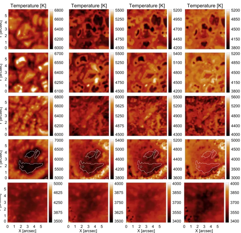
Figure5shows horizontal cuts of the plasma temperature in the various observed regions at four different heights, specifically atlogt500=0,−1.5, −2, and −2.5. The various panels display plasma temperatures that decrease with atmo-spheric height for all the analyzed regions. The top panels show the reversed granular pattern already at anatmospheric height oflogt500= -1. The same applies to the pattern of BPs, and to alesser extent, also to pattern of PL regions.

3.2. Response Functions and Uncertainty

In order to assess the range of atmospheric heights in which the analyzed data are sensitive to temperature perturbations, thus to specific properties of the observed atmosphere, we computed the

Figure 2.Top panel: Stokes-I spectra from measurements(OBS) of QS regions and those from SA data inversion using different starting guess models, specifically the HSRA, VAL-C, and FAL-C-99 models. Bottom panel: relative difference between synthetic and observed spectra.

Figure 3.As in Figure2, but for measurements(OBS) and SA data inversion results concerning the PL region. The HSRA, VAL-C, and FAL-P-99 models have been tested here as guess models.

so-called response functions(RFs, e.g., Caccin et al.1977; Landi Degl’Innocenti & Landi Degl’Innocenti 1977) by applying the

mathematical procedure described in Socas-Navarro (2011).

Figure6shows the RFs based on the results of the SA inversion of QS data, i.e., inversion of data averaged over the studied subFOV, normalized to the maximum value. For a given Stokes parameter, optical depth, and wavelength, RFs values close to unity indicate that the corresponding Stokes-parameter measure-ments are quite responsive to perturbations of the line-forming atmosphere, while low or null RFvalues signifythat the Stokes measurements are unaffected by atmospheric inhomogeneities of temperature andfields. This implies that the data inversion cannot provide reliable information about the physical quantities in the line-forming atmospheric regions that arecharacterized by low

RFs values; these regions lie outside the sensitivity range of theanalyzed data. Figure 6 shows thatfor the observations considered in our study, the sensitivity range spans from

t =

log 500 0 tologt500= -3. The variation in

emerginginten-sity that isdue to temperature perturbations is always positive: the emergingintensity increases inboththe continuum andthe line core, with most of the contribution to the analyzed spectra coming from the continuum.

Following Socas-Navarro (2011), we also computed the

uncertainty in the atmosphere models derived from the data inversionby weighting the average of the temperature stratification ( tT( ), hereafter) obtained from the inversion at each observed spectral point by the above estimated RFs. Figure7 shows the uncertainty estimated for theT( )t derived

Figure 4.From left to right, top to bottom: horizontal cuts of the temperature, magneticfield strength, plasma density, and LOS velocity atlogt500=0on the atmosphere models derived from inversion of the QS, BPs, PL, PO, and UM regions. White and black contours mark the PO region considered to compute the average temperature profiles labeled (a) and (b) in Figure10.

from thefive inverted subFOVs. This uncertainty is as low as ∼15 K betweenlogt500=0andlogt500= -3, i.e., the range

of atmospheric heights in which the data inversion returns more reliable results. The uncertainty of thedata inversion results increases at higher atmospheric heights and belowlogt500=0, up to 50 K and 200 K, respectively, as well as with decreasingspatial scale of the magnetic feature represented by the inverted subFOV.

3.3. Temperature Stratification

We compared theT( )t derived from the data inversion of the various studied regions to thosedescribed by the several 1D models listed in Table1. We here consider results obtained

from inversion of data taken at best seeing conditions for each analyzed region and for both the SA and FR computations.

Figure 8 (top panel) shows this comparison for QS data.

Dashedand solidblack lines display theT( )t obtained from SA and FR, labeled (a) and (b), respectively. Colored lines correspond to the 1D models employed for comparison as specified in the legend. The gray-shaded area represents the 1σ confidence interval of data inversion results. Figure8 (bottom

panel) shows the relative difference between theT( )t derived from the observations and from a 1D model used as reference, specifically, the FAL-C-99 model.

The panels in Figures9 and 10 show the same content as Figure8, but based on the results obtained from the inversion of the BPs, PL, PO, and UM observations. The bottom part in

Figure 5.From left to right, top to bottom: horizontal cuts of the temperature at four different heights, specifically atlogt500=0,-1.5,- -2, 2.5, derived from the inversion of the QS, BPs, PL, PO, and UM data. See caption of Figure4for more details.

each panel shows the relative difference between the T( )t derived from the observations and from the 1D model used as reference, which is the FAL-(F, P, S)-99 to represent network, plage, and umbral regions, respectively; we also analyzed the FAL-R-06 model for penumbral regions.

Concerning the PO data, we considered results from SA and FR computations on the image pixels with Ic<0.4 (labeled (a)-dark and (b)-dark, respectively), and over the whole subFOV (labeled (a) and (b), respectively). We then estimated the relative difference between theT( )t computed over the whole subFOV and the FAL-R-06, as well as between theT( )t computed over the image pixels with Ic<0.4and the FAL-S-99.

Figures 8–10 show that the various T( )t derived from the data inversion agree quite well with those in most of the compared models, both qualitatively and quantitatively, exceptfor PO observations. The agreement between compared models decreases outside the sensitivity range defined by the RFs; we recall, however, that outside the sensitivity range the physical quantities returned by the data inversion are uncertain. For all studied regions, the T( )t obtained from SA and FR computationsdiffer slightly. We discuss this difference in the

following and mostly focus here on results from FR computations alone.

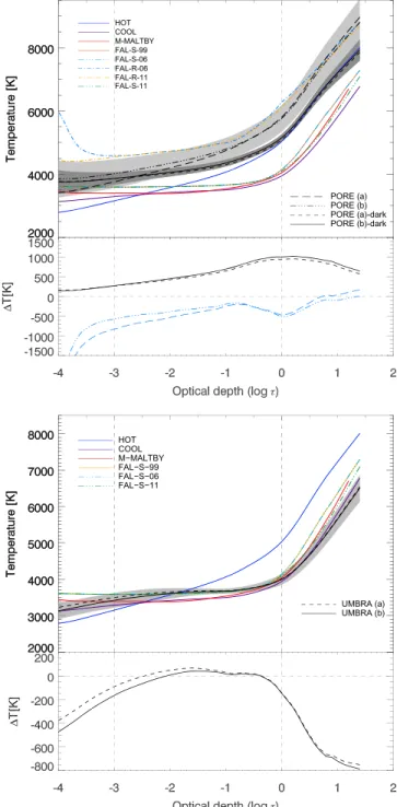
At logt500=0, the average of the temperature values obtained from the inversion of the QS, BPs, PL, andUM data agree with those in the FAL-(C, F, P, S)-99 models within the deviation of results on the analyzed subFOV, wherethe average and standard deviation of values is 6383±132K, 6397±132 K, 6427±132K, and 3998±150K with respect to the values 6520K, 6520K, 6502K, 4170K in the FAL-(C, F, P, S)-99 models, respectively. At same atmospheric height, the value of the plasma temperature estimated by the inversion of PO data is 5147±109 K, ∼1000 K higher and ∼1100 K lower than the values consideredin the FAL-S-99 and FAL-R-06 models, respectively. The relative difference between ourT( )t derived from analysis of the whole subFOV and the FAL-R-06 model is less pronounced; theT( )t of the FAL-R-06 model lies within the deviation of values derived from our analysis, in the atmospheric range betweenlogt500= -0.5andlogt500= -2.

Within logt500= -1 and logt500= -3, i.e., from the

middle to the high photosphere, the T( )t returned from the observations of QS, BPs, PL, and UM regions agree within ∼10% with all theT( )t in the models by Fontenla et al.(1999)

employed for comparison, but with slightly different results for the various compared sets; for QS, BPs, and UM regions, the agreement is within 5%, while for the PL regions it iswithin 10%. Overall, most of theT( )t derived from the data inversion are slightly lower than thosein the compared 1D models in the middle photosphere(about 100K atlogt500= -1) and slightly higher in upper layers(about 150K atlogt500= -3) and below

t =

log 500 0 (about 200–400K), but for the UM data, which

Figure 6.Normalized RFs of the Stokes-I to temperature perturbation derived from analysis of the QS observations.

Figure 7.Temperature uncertainties for each analyzed region, as specified in the legend.

Figure 8.Top: Comparison oftheT( )t of several 1D models(colored lines, as specified in the legend) and in the model derived from the inversion of the QS observations. The gray-shaded area represents the 1σ confidence interval of thedata inversion results. Dashed and solidblack lines refer to the T( )t retrieved from the SA and FR computations, labeled(a) and (b), respectively. Bottom: Relative difference between theT( )t retrieved from the data inversion and from the FAL-C-99 model. The horizontaldashed line marks zero values of these differences; theverticaldashed lines in both panels mark the sensitivity range defined by the RFs.

show lower plasma temperatures (down to 700K) below

t =

log 500 0 than those displayed by all compared models, and the PL data, which exhibit lower values(about 50−100 K) above

t =

-log 500 2.5than all other models. In particular, the T( )t obtained from QS and BPs data are, on average, up to∼100K lower than in the corresponding FAL-C-99 and FAL-F-99 models. In the range between logt500=0 and logt500= -2,

i.e., in the lower and middle photosphere, theT( )t obtained from PL data is, on average, up to∼400 K lower than represented in the corresponding FAL-P-99 model. On the other hand, at these atmospheric heights, the T( )t from PO observations is up to ∼1000 K higher than reported by the FAL-S-99 model; for the UM data, it is close(within ∼50–100 K) to that described in the

FAL-S-99 model, but it is ∼150–200 K lower atlogt500=0 andlogt500= -3.

All the atmosphere models derived from the observations exhibit higher plasma temperatures at higher atmospheric heights than those represented by the earlier HSRA and VAL-C models, except for the model derived by the PL data. In addition, the T( )t obtained from BPs and PL datado not reproduce the temperature enhancement represented in the SOLANNT and SOLANPL models either, neither for the SA nor for the FR results. TheT( )t from theSA analysis of PL

Figure 9.As in Figure8, but for data representative of small-scale(BPs, top) and large-scale(PL, bottom) bright magnetic regions. The relative difference is computed with respect to the temperature stratification of the FAL-F-99 (top) and the FAL-P-99(bottom) models. See caption of Figure8for more details.

Figure 10.As in Figure8, but for data representative of dark magnetic regions, PO(top) and UM (bottom). For PO data, labels (a) and (b) refer to theT( )t computed over the whole subFOV, while labels(a)-dark and (b)-dark refer to theT( )t over the region withIc<0.4. The relative difference is computed with respect to the temperature stratification of the FAL-R-06 (dot-dashed and long-dashed lines) and the FAL-S-99 (solid and dashed lines) models, respectively. See caption of Figure8and Section3for more details.

data most closely follows the FAL-P-93 and FAL-H-99 models.

Atmosphere models derived from observations seem to reproduceformer models by Fontenla et al. (1993, 1999)

betterthan more recent sets by Fontenla et al. (2006,2011), at

least in the lower photosphere up tologt500= -2, and mainly for QS and BPs regions. The opposite seems to occur in upper atmospheric layers, wherethe confidence levelof our data inversion results is lower, however.

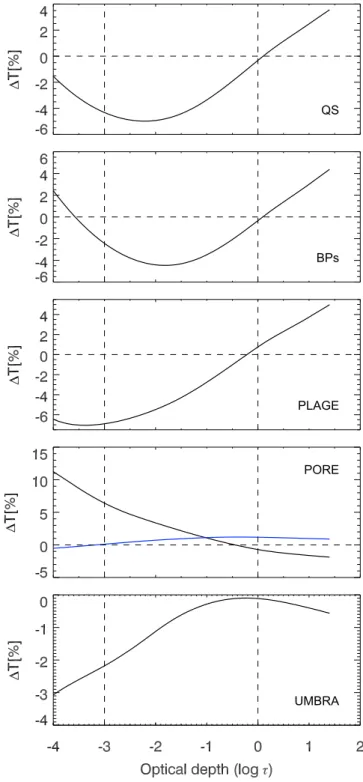
3.4. Effects of Spatial Averaging and Temporal Evolution Figures 8–10 show slight differences between the T( )t obtained from SA and FR computations, i.e., the spatially averaged and fully resolved observations. In Figure 11 we quantify this differenceby showing relative percentage values between the T( )t obtained under the two computations applied; for PO regions we also show results from ananalysis of image pixels with Ic<0.4. At logt500=0, the difference

betweenT( )t obtained from SA and FR lies within 1% for all the analyzed regions. For PO and UM data, the difference is within 2% at all the investigated atmospheric heights whenwe restrict our analysis to image pixels with Ic<0.4.

Within logt500=0 and logt500= -3, i.e., from the lower

to the higher photosphere, for QS, BPs, and PL regions, the

t

( )

T computed from SA on the whole subFoV has up to 6% higher values than obtained from FR, while for the PO theT( )t has up to;6% lower values; for UM, theT( )t computed from SA on the whole subFOV has only up to 2% higher values than obtained from FR. Therefore, the results obtained from bright and dark magnetic regions are similarlyaffected by the method applied, except forthe sign for PO observations; this holds whenthe analyzed data are characterized by a spatial resolution of ≈5–6 arcsec as considered in our study.

The above results indicate that the method applied affectsthe modeled atmosphere in homogeneous magnetic regions less. This is in agreement with Uitenbroek & Criscuoli (2011), who showed that spatially averaging the properties of

an inhomogeneous atmosphere returned from MHD simula-tions and evaluating physical quantities after the averaging operationdoes not give the same result as estimating the physical quantities in the inhomogeneous atmosphere and then averaging it.

We also investigated the possible effects that aredue to the temporal evolution of the observed features on the obtained resultsand other possible processes occurring in the analyzed regions (waves, seeing, etc.). To this purpose, we analyzed inversion results derived from SA computations on the whole series of data available for each observed region. In Figure12

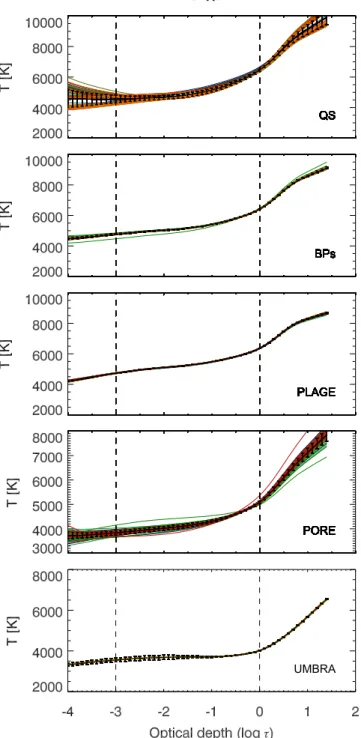
we show theT( )t derived from the inversion of all averaged Stokes spectra for each observed region. The T( )t retrieved from ananalysis of each observation available for the studied region is displayed with different colors. The T( )t averaged over the whole time series is displayed as a solidblack line with error bars representing the 1σ confidence interval; this interval is larger for QS and PO regions. Figure 12shows that the dispersion of results that isdue to the effects of the temporal evolution of the studied region and other possible processes lies within the confidence interval of theresults estimated for all the analyzed regions. Thisfinding proves that the results presented in Sections3.1–3.3can be assumed to be quite representative of the studied regions, at least for the data set considered in our study.

4. Comparison with Results in the Literature The literature presents a number of atmosphere models derived from inversion of spectropolarimetric data acquired with both ground-based and space-borne instruments. We now discuss theT( )t derived from our analysis with respect to those reported by former studies of QS, PL, and UM regions. We focus on the models presented since2000 that werederived from ananalysis of data taken with similar characteristicsin

Figure 11.From top to bottom: Relative difference between the averageT( )t obtained from ananalysis of fully resolved (FR) and spatially averaged (SA) results from inversion of the QS, BPs, PL, PO, and UM data. The blue line in the panel of PO data shows results obtained by considering only image pixels withIc<0.4.

terms of spatial and spectral resolutionas those considered in our study.

Borrero & Bellot Rubio (2002) presented a two-component

model of the quiet solar photosphere that isrepresentative of typical granular and intergranular regions, derived from aninversion performed with the SIR code on the intensity of 22 FeI lines that wereobserved withthe Fourier Transform Spectrometer(FTS) installed at the McMath telescope of the Kitt Peak Observatory. The data consist of 1579 spectral points that sample the 22 selected FeI lines at intervals of 6mÅ. At

t =

log 500 0, the plasma temperature derived from our analysis of the QS observations is comparatively close to the values in both their models, with relative differences of ∼100K. Given

consecutive scans of 315 slit positions on the FoV, each position with 112 wavelength samples of the FeIline pair taken with 21 mÅ sampling. The inversion was performed on a subarray of about 30×30 arcsec2, 200×200 pixels wide. The retrieved average temperature stratification was compared to the HSRA and the model by Asplund et al.(2004), which

was foundto be warmer in the middle layers thanthe model presented in Socas-Navarro (2011) and cooler upward; it is

very close to that obtained from our analysis of FR QS data, exceptfor the elbow atlogt500= -1that is not foundin our resultsor in the HSRA model. The uncertainties derived from RFs by Socas-Navarro (2011) exhibit a similar trend as

thosederived from our study, at least for image pixels with acontinuum brightness close to the average of the whole observed region. For these pixels, the uncertainties estimated by Socas-Navarro (2011) are lower than 50 K in the middle

atmospheric layers, up to logt500= -3.4, and reach values ofup to more than 500 K in the upper layers. These values are sensitively higher than those derived from our study.

Bellot Rubio et al. (2000) analyzed averaged Stokes-I and

Stokes-V spectra of the FeI line pair at 630 nm thatemerged from a facular region observed at μ=0.96 with the slit Advanced Stokes Polarimeter (ASP) at the Sacramento Peak Observatory. The observations, which covered a FoV of about 110×90arcsec2, were taken in almost 20 minutes. The spatial resolution of the acquired data was ;1–3 arcsec and the spectral sampling was 13 mÅ. The analyzed data consist of averaged Stokes profiles constructed by accounting for the contribution of all pixels within facular regions whose degree of polarization was lower than 0.4%. The model they presented for the central part of the studied region is hotter than the model we obtained from the PL data,∼500 K hotter atlogt500=0. OurT( )t better agrees with the one reported by Bellot Rubio et al. (2000) for the atmosphere surrounding the magnetic

facular region. However, the T( )t obtained from our study agrees with their results within the standard deviation of values in our studied subFOV.

Buehler et al. (2015) analyzed the full-Stokes spectra of a

plage region observed at the FeI line pair at 630 nm with the slit spectropolarimeter onboard the Hinode missionusing the revised version of the SPINOR inversion code (Frutiger et al. 2000), whichallowsaccounting for the instrumental

point-spread functions (van Noort 2012). The observations

covered a FoV of about 50×150 arcesec2, acquired with a spatial resolution of 0.32 arcsec and spectral sampling of 21 mÅ over about 5 minutes. The T( )t they reported for core regions, defined as the image pixels with magnetic field strength decreasing with height and absolute value>1000 G,

Figure 12.From top to bottom:T( )t obtained from the analysis of the whole series of available QS, BPs, PL, PO, and UM observations. Each temporal step in the observational series is shown with adifferent color. Error bars indicate the standard deviation of values with respect to theT( )t averaged over the whole time series, shown as ablacksolid line.

shows comparatively higher values (up to ∼600 K) than obtained from our study; their values are closer to the empirical plageflux-tube model derived by Solanki & Brigljevic (1992),

at least up to logt500= -1, compared to ours. Nevertheless, the results they obtained for the average temperature of pixels representative of QS and magnetic field concentrations at

t = -

-log 500 0, 0.9, 2.3are in good agreement with thosewe obtained from the inversion of QS and PL data, within the deviation of results in the analyzed subFOV.

Westendorp Plaza et al. (2001) studied full-Stokes spectra

taken at the FeIline pair at 630 nm on a sunspot region with the slit ASPusing the SIR code. They computed the RFs of Stokes-V to the perturbation of the magneticfield strength, and deduced a sensitivity range spanning betweenlogt500=0and

t =

-log 500 2.8, in good agreement with our estimation of the sensitivity range of the studied data. They also derived the confidence limits for the retrieved stratification of physical parameters from the computation of RFs, and verified that the errors obtained were in good agreement with Monte Carlo simulations. Their estimated formal errors are comparable tobut sligthly larger than our computed uncertainties for results from the PO and UM data.

Analysis of key aspects of the studies described above shows that our work benefits from a higher spectral and spatial resolution of the analyzed observations, and a wider data set taken under excellent seeing conditions than considered in all previous studies. We also discuss our results with respect to a significantly larger set of 1D models than earlier presented in the literature. In addition, within the computational uncertainty of results, all findings derived from our study are consistent with results of the above earlier works. Thus, the results derived from our study can reasonably be assumed to represent the analyzed regions.

5. Application to SI Studies

The set of 1D models employed in semi-empirical SI reconstructions is of pivotal importance to reproduce measured SI variations accurately(see e.g., Ermolli et al.2013). It is thus

interesting to test the accuracy of the observation-based atmosphere models derived from our study for possible application in SI models.

In order to provide a preliminary assessment of such accuracy, we computed the radiative flux emerging from our observation-based atmospheres and compared it with the fluxresulting from other 1D models employed in semi-empirical SI models, and with other available data that are described below. We performed the spectral synthesis for the wavelength range from 200 to 2400 nm on the various analyzed atmospheres with the one-dimensional version of the RH code (Uitenbroek 2001), which solves the RT and statistical

equilibrium equations under general NLTE conditions. We computed the emergingspectrum with a 0.01 nm spectral resolution at nine lines of sight, spaced according to the zeroes of the Gauss-Legendre polynomials as a function ofμ. We then convolved the spectra derived from the synthesis with a Gaussian kernel 1 nm wide, to roughly account for the spectral resolution of the SI data considered for comparison.

We applied standard NLTE RH computations, which consider contributions of Thomson scattering by free electrons, Rayleigh scattering by neutral hydrogen and helium atoms, and H2molecules. Other background opacity sources included were

bound-free and free-free transitions of H− and neutral

hydrogen, free-free transitions of H2,and bound-free

transi-tions of different metals. The synthesis was performed by computing populations of several atoms2and of more than 10 molecules.3We assumed the atomic line data from Kurucz.4

Figure13(top panel) shows the SI spectra derived from the

synthesis performed on the QS and FAL-C-99 models representative of QS regions, compared to the ATLAS-3 reference spectrum by Thuillier et al.(2004), Figure13(middle

and bottom panels) displays the relative difference of the synthesized spectra with respect to the above reference data. The ATLAS-3 is a composite solar spectrum derived from analysis of various available measurements; it is considered a standard reference for SSI covering the UV (200–300 nm), near-UV(NUV, 300–400 nm), visible (Vis, 400–700 nm), and near-IR (NIR, 700–2400 nm) spectral regions. In the Vis and NIR bands, the median(standard deviation) relative difference between the SI spectrum derived from our QS atmosphere and reference data is;0.8% (4%) and −3% (1.9%), respectively; the median(standard deviation) relative difference between the compared spectra, however, increases up to 13% (14%) and 85%(>100%) in the NUV and UV regions, respectively. In the Vis and NIR bands, the median (standard deviation) relative difference between the SI spectrum derived from our synthesis on the FAL-C-99 model and reference data is;6% (4%) and −0.3% (2%), respectively; the median (standard deviation) relative difference between these compared spectra increases up to 22% (17%) and 140% (>100%) in the NUV and UV regions, respectively.

Figure 13.Top panel: SI from 200 to 2400 nm calculated with our spectral synthesis performed on the QS and FAL-C-99 atmospheres representative of QSregions and measured reference data by Thuillier et al. (2004). Middle and

bottom panels: relative difference between the SI derived from the synthesis on the QS (middle) and FAL-C-99 (bottom) atmospheres with respect to the reference data. SI data are given in [W m−2nm−1] units. All spectra were convolved with a 1 nm Gaussian kernel to account for the spectral resolution of available measurements in the visible range. The solid lines in themiddle and bottom panels show relative differences between the data convolved with a 10 nm Gaussian kernel. Vertical lines mark the UV, NUV, Vis, and NIR bands.

2

Including H, C, O, Si, Al, Ca, Fe, He, Mg, Na, N, andS.

3

Including H2,H+2, C2, N2, O2, CH, CO, CN, NH, NO, OH, SiO, LiH,

andMgH.

4

Other available spectra from SI models show arelative difference with respect to the ATLAS-3 data such as those reported above. Ofthe various models developed to reproduce the SI variability, we considered those that aremost representa-tive of the two classes introduced in Section 1, the proxy NRLSSI model (Lean2000; Coddington et al. 2016), and the

semi-empirical SATIRE-S model(e.g., Yeo et al.2014a,2014b, and references therein).

Figure 14(top panel) shows the SI spectrum derived from

our synthesis performed on the QS atmosphere, compared to the SI spectrum computed with the Kurucz QS model and to the WHI reference data by Woods et al.(2009), which give the

QS spectrum in the SATIRE-S and NRLSSI SI models, respectively. Figure14(middle and bottom panels) displays the

relative difference between the SI spectrum from the QS atmosphere and the WHI datawith respect to the SI spectrum calculated with the Kurucz QS model, which is employed in the SATIRE-S model. This isthe currentlymostadvanced semi-empirical SI model. The SI spectrum derived from the QS atmosphere (described by WHI) shows amedian relative difference to the spectrum computed in the Kurucz atmosphere model of ;34%, 6% 0.7%, and −0.6% (−32%, −11%, −0.2%, and3%) in the UV, NUV, Vis, andNIR bands, respectively.

In order to highlight the main features of the SI data compared above, we also show in Figure 15 the relative difference between the various available spectra with respect toATLAS-3, after spectral convolution of the data with a Gaussian kernel 10 nm wide, in order to display average trends over the various spectral regions. In the Vis, the agreement ofthe compared spectra is very good, ranging from −0.14% (Kurucz model in SATIRE-S) to 6% (FAL-C-99) for all the data analyzed; themedian relative difference is 0.8%, 6%, −0.1%, and −0.3% for QS, FAL-C-99, Kurucz, and WHI,

respectively. In the NUV range, thisagreement decreases to ;13% and 22% for our QS and FAL-C-99 computations, while it decreases only to≈−6% and 6% for the data considered in the NRLSSI and SATIRE-S models. It is worth nothing that these latter models estimate the time- and wavelength-dependent contribution to SI from bright and dark magnetic features in quite different ways, but both apply intensity offsets and some scaling forthe reconstructed SI spectra tomatch the absolute levels of some observed reference spectra. In addition, the spectral synthesis performed in the SATIRE-S assumes LTE conditions that fail to reproduce the SI below 300 nm accurately. Outcomes from the SATIRE-S synthesis are rescaled to reference data by Woods et al.(2009). In contrast,

the results of the spectral synthesis performed on our observational-based QS atmosphere and the FAL-C-99 model shown in Figure 15 are taken as they are from our RH calculations, without applying any scaling to improve the match to the reference data by Thuillier et al.(2004).

We also analyzed the spectra derived from the synthesis on the observation-based BPs, PL, PO, and UM models, with respect to thoseobtained from the synthesis on the FAL-(E, F, H, S)-99 and FAL-R-06 models. This comparison shows higher relative differences in the UV than in the other spectral bands. Specifically, in the UV and NUV, the various spectra differon average by;15% and 80% for models of bright and dark features, respectively; in the Vis (NIR) they differon averagefrom 0.3% to 2% (0.04%–1.6%) for models of bright features, and from 11 to>250% (7%–60%) for models of dark features. These differences affect calculations of the SSI that arebased on the various compared models as summarized in Table2. We report in Table2the SSI computed by integrating the various synthesized spectra from 200 to 2400 nm; we also show the relative difference between SI computed for models corresponding to thesame surface feature. The relative difference between the computed SSI ranges from −0.5% (PL with respect to FAL-F-99 computations) to 93% (P0 with respect to FAL-R-06 computations). Except forthese extremes,

Figure 14. Top panel: SI from 200 to 2400 nm derived from our spectral synthesis performed on the QS atmosphere, calculated with the Kurucz QSmodel employed in the SATIRE-S SI model, and given by the WHI reference data considered in the NLRSSI SI model. Middle and bottom panels: relative difference between the SI derived from the synthesis on the QS atmosphere (middle) and considered in the NRLSSI model (bottom) with respect to the SI calculated with the Kurucz QSmodel employed in the SATIRE-S. See caption of Figure13for more details.

Figure 15. Relative difference between the SI spectra derived from our synthesis on the QS and FAL-C-99 atmospheres, and computed with the Kurucz QSmodel employed in the SATIRE-Swith respect to the reference data from Thuillier et al.(2004) and WHI by Woods et al. (2009), the latter

considered in the NRLSSI model. See caption of Figure13and Section5for more details.

the best(worse) agreement between the compared quantities is found for the SSI that iscomputed on the BPs and the FAL-E-99 atmospheres(PO and FAL-S-99 atmospheres).

It is worth nothing that the values in Table2result from the synthesis performed on the atmosphere models presented in Section 3. In our study, we assumed that these data satisfactorilyrepresent atmosphere regions employed in SI reconstructions. However, the subFOVs analyzed in our observations represent only a minute fraction of the solar disk at a given time, while the solar regions thatthe data are assumed to represent can cover significant fractions of the solar disk and show different brightness in time. For some surface features, the results derived from our study may not accuratelyreflect the properties of the modeled atmosphere. This is especially the case when rather inhomogenous regions are considered. For example, we show in Figure16results from the synthesis performed in the three PL regions that aremarked with red and blue boxes in Figure1. TheT( )t derived from the blue marked regions show slightly different average values than obtained from theanalysis of the red marked region. In particular, theT( )t of the PL region discussed in Section3lies between thoseobtained from the other two analyzed PL areas. The SI spectra derived from the synthesis on the three PL atmospheres differ on average by;10%, 5%, and <5% in the UV, NUV, and Vis ranges, respectively. When entered in SI models, these differences translate into SSI estimated values that differ from 1.1% to 2.6%.

The above results encourage us to further investigate the accuracy of entering atmosphere models derived from spectro-polarimetric observations in SI estimates. Indeed, the Vis and NIR SSI synthesized on the atmosphere model derived from our QS observations differs on average from the ATLAS-3 and WHI reference data byless than 2.5%, and −0.14% from the spectrum computed on the Kurucz QS atmosphere employed in the SATIRE-S model. In addition, the lower agreement reported above for synthesis results of the NUV and UV bands, below 400 nm, is fully consistent with the limited range of atmospheric heights sampled by the data analyzed in the present study, which spans from the low to the high photosphere only, thus limiting the reliability of our spectral synthesis results for the SI originating from higher atmospheric heights. On the other hand, in the 1000–2400 nm spectral region, the SI derived from our synthesis on the QS atmosphere underestimates (−3.5% ± 1.5%) the reference dataas a con-sequence of the clear SSI drop seen at about 1000 nm. This drop challenges our synthesis calculations of theH opacity for -the NIR range. Indeed, in -the same spectral region, results derived from our synthesis on the FAL-C-99 atmosphere by

assuming the H population data available for that model differon average byonly −0.7% with respect to the reference. However, it is also worth noting that several recent NIR SI measurements show a systematic negative difference(of about 8%) with respect to the ATLAS-3 reference composite, see e.g., Weber(2015), in agreement with our findings.

6. Discussion and Conclusion

We found that the average temperature stratification derived from the data inversion of the various analyzed regions agrees well with that represented by the corresponding 1D model, both qualitatively and quantitatively, exceptfor pore data, which exhibita different trend at all atmospheric heights compared to the 1D models that arerepresentative of umbral regions. This result is not surprising, since previous studies already strengthened the linear dependence of umbral core brightness on their size (e.g., Collados et al.1994; Mathew et al. 2007).

These latter results, however, suggest that the 1D models employed in current SI reconstructionsmay inaccurately represent the temperature stratification of darkmagnetic regions thatare neither spatially extended nor characterized by strong magneticfields as typical umbral regions. Moreover, such features are not accounted for in the atmosphere models of dark structures employed in SI reconstructions. Our results also suggest that pixel-by-pixel inversion of high-resolution obser-vations allowsretrievingatmosphere models that possibly better account for the contribution of the smaller-scale features in the studied FoVthan obtained from ananalysis of less well resolved observations. This is particularly interesting, since SI cyclic variations are closely linked to the evolution of small-scalestrong-field magnetic features.

Our preliminary investigation of the accuracy of potentially entering the various atmosphere models derived from our study in SI estimates gave encouraging results. Indeed, the SI spectrum from 400 to 2400 nm synthesized on the atmosphere model derived from our QS observations differs on average by 2.2% from the ATLAS-3 reference data by Thuillier et al. (2004)and by - 0.14% from the spectrum computed in the

Kurucz QS atmosphere employed in the SATIRE-S SI model. In the same spectral range, the median difference between the

Table 2

Spectrally Integrated Flux from 200 to 2400 nm Computed from the Observation-based Atmospheres and the FAL-(C, E, F, H, S)-99

and FAL-R-06 Models

Obs SSI Obs Model SSI FAL Rel. Diff.

Region [W m2_{] Label [W m}2_{] [%]} QS 1354.60 C 1416.85 4.6 BP 1404.10 E 1426.06 1.6 PL 1453.55 F 1446.77 −0.5 PL 1453.55 H 1510.46 3.9 PO 624.24 R 1205.53 93 PO 624.24 S 303.36 −51 UM 273.57 S 303.36 11

Figure 16.SI from 200 to 400 nm(top), and from 400 to 700 nm (bottom), derived from the synthesis on the atmosphere models of three PL regions and BPs area shown in Figure1.

properly enter synthesis results of observation-based models in SI reconstructions, a more detailed study is also required to account for the center-to-limb dependence of the intensity emerging from features that areobserved at different positions on the solar disk, and for the different brightness of each magnetic feature depending on the magnetic filling factor. However, preliminary tests of the accuracy of the outcomes derived from the present study, by using data representative of other solar regions that also cover wider ranges of atmospheric heights than discussed above, have given promising results that motivate us to further work for the exploitation of atmosphere models that arederived from inversion of spectropolarimetric observations in SI reconstructions.

The authors wish to thank the referee, Kok Leng Yeo, for fruitful comments that helped them improve the manuscript. They are also thankful to Gianna Cauzzi, Serena Criscuoli, Valentina Penza, Hector Socas-Navarro, Sami Solanki, and Han Uitenbroek for useful discussions and advice for the data inversion and synthesis computations, and to the International Space Science Institute, Bern, for the opportunity to discuss this work with the team“Towards a Unified Solar Forcing Input to Climate Studies” lead by Natasha Krivova. This study received funding from the European Unions Seventh Programme for Research, Technolo-gical Development and Demonstration, under the Grant Agree-ments of the SOLARNET (n 312495,http://www.solarnet-east. eu) and SOLID (n 313188, projects.pmodwrc.ch/solid/) projects.

This work was also supported by the Istituto Nazionale di Astrofisica (PRIN-INAF-2014) and Italian MIUR (PRIN-2012).

References

Asplund, M., Grevesse, N., Sauval, A. J., Allende Prieto, C., & Kiselman, D. 2004,A&A,417, 751

Bellot Rubio, L. R. 2003, in ASP Conf. Ser. 307, Solar Polarization, ed. J. Trujillo-Bueno & J. S. Almeida(San Francisco, CA: ASP),301

Bellot Rubio, L. R., Ruiz Cobo, B., & Collados, M. 2000,ApJ,535, 489

Borrero, J. M., & Bellot Rubio, L. R. 2002,A&A,385, 1056

Buehler, D., Lagg, A., Solanki, S. K., & van Noort, M. 2015,A&A,576, A27

Caccin, B., Gomez, M. T., Marmolino, C., & Severino, G. 1977, A&A,54, 227

Coddington, O., Lean, J., Rottman, G., et al. 2016, in EGU General Assembly Conf. Abstracts 18(Vienna: Copernicus),9026

Collados, M., Martinez Pillet, V., Ruiz Cobo, B., del Toro Iniesta, J. C., & Vazquez, M. 1994, A&A,291, 622

358, 1109

Gingerich, O., Noyes, R. W., Kalkofen, W., & Cuny, Y. 1971, SoPh,

18, 347

Haigh, J. D. 2007,LRSP,4, 2

Kopp, G. 2016,JSWSC,6, A30

Krivova, N. A., Solanki, S. K., & Floyd, L. 2006,A&A,452, 631

Kurucz, R. L. 1993, IAUCB,21, 93

Kurucz, R. L. 2005, MSAIS,8, 189

Landi Degl’Innocenti, E., & Landi Degl’Innocenti, M. 1977, A&A,56, 111

Landi Degl’Innocenti, E., & Landolfi, M. 2004, Polarization in Spectral Lines, Vol. 307(Dordrecht: Kluwer)

Lean, J. 2000,GeoRL,27, 2425

Lean, J. L., Rottman, G. J., Kyle, H. L., et al. 1997,JGR,102, 29939

Maltby, P., Avrett, E. H., Carlsson, M., et al. 1986,ApJ,306, 284

Mathew, S. K., Martínez Pillet, V., Solanki, S. K., & Krivova, N. A. 2007,

A&A,465, 291

Piskunov, N. E., Kupka, F., Ryabchikova, T. A., Weiss, W. W., & Jeffery, C. S. 1995, A&AS,112, 525

Requerey, I. S., Del Toro Iniesta, J. C., Bellot Rubio, L. R., et al. 2014,ApJ,

789, 6

Rottman, G. 2006,SSRv,125, 39

Ruiz Cobo, B., & del Toro Iniesta, J. C. 1992,ApJ,398, 375

Scharmer, G. B., Dettori, P. M., Lofdahl, M. G., & Shand, M. 2003,Proc. SPIE,4853, 370

Scharmer, G. B., Narayan, G., Hillberg, T., et al. 2008,ApJL,689, L69

Shchukina, N., & Trujillo Bueno, J. 2001,ApJ,550, 970

Socas-Navarro, H. 2011,A&A,529, A37

Socas-Navarro, H., de la Cruz Rodríguez, J., Asensio Ramos, A., Trujillo Bueno, J., & Ruiz Cobo, B. 2015,A&A,577, A7

Solanki, S. K. 1986, A&A,168, 311

Solanki, S. K., & Brigljevic, V. 1992, A&A,262, L29

Solanki, S. K., Krivova, N. A., & Haigh, J. D. 2013,ARA&A,51, 311

Stangalini, M., Giannattasio, F., & Jafarzadeh, S. 2015,A&A,577, A17

Thuillier, G., Floyd, L., Woods, T. N., et al. 2004, in Solar Variability and its Effects on Climate. Geophysical Monograph, Vol. 141 ed. J. M. Pap et al. (Elsevier: New York),171

Uitenbroek, H. 2001,ApJ,557, 389

Uitenbroek, H., & Criscuoli, S. 2011,ApJ,736, 69

Unruh, Y. C., Solanki, S. K., & Fligge, M. 1999, A&A,345, 635

van Noort, M. 2012,A&A,548, A5

van Noort, M., Rouppe van der Voort, L., & Löfdahl, M. G. 2005,SoPh,

228, 191

Vernazza, J. E., Avrett, E. H., & Loeser, R. 1981,ApJS,45, 635

Weber, M. 2015,SoPh,290, 1601

Westendorp Plaza, C., del Toro Iniesta, J. C., Ruiz Cobo, B., et al. 2001,ApJ,

547, 1130

Woods, T. N., Chamberlin, P. C., Harder, J. W., et al. 2009, GeoRL,36, L01101

Yeo, K. L., Krivova, N. A., & Solanki, S. K. 2014a,SSRv,186, 137

Yeo, K. L., Krivova, N. A., Solanki, S. K., & Glassmeier, K. H. 2014b,A&A,