Reconstruction of vehicle dynamics from inertial and GNSS data

(1)

ALMA

MATER

STUDIORUM

_·

UNIVERSITÀ DI

BOLOGNA

Reconstruction of vehicle dynamics

from inertial and GNSS data

Scuola di Scienze

CORSO DI LAUREA IN INFORMATICA

Supervisor: Chiar.mo Prof. Stefano Sinigardi Co-Supervisor:

Dott. Alessandro Fabbri

Candidate: Federico Bertani

I sessione

(2)

(3)

A

BSTRACT

The increasingly massive collection of data from various types of sensors installed on vehicles allows the study and reconstruction of their dynamics in real time, as well as their archiving for subsequent analysis. This Thesis describes the design of a numerical algorithm and its implementation in a program that uses data from inertial and geo-positioning sensors, with applications in industrial contexts and automotive research. The result was made usable through the development of a Python add-on for the Blender graphics program, able to generate a three-dimensional view of the dynamics that can be used by experts and others. Throughout the Thesis, particular attention was paid to the complex nature of the data processed, introducing adequate systems for filtering, interpolation, integration and analysis, aimed at reducing errors and simultaneously optimizing performances.

La raccolta sempre più massiccia di dati provenienti da sensori di varia natura installati sui veicoli in circolazione permette lo studio e la ricostruzione della loro dinamica in tempo reale, nonché la loro archiviazione per analisi a posteriori. In questa Tesi si descrive la progettazione di un algoritmo numerico e la sua implementazione in un programma che utilizza dati provenienti da sensori inerziali e di geo-posizionamento con applicazioni a contesti industriali e di ricerca automobilistica. Il risultato è stato reso fruibile tramite lo sviluppo di un add-on Python per il programma di grafica Blender, in grado di generare una visualizzazione tridimensionale della dinamica fruibile da esperti e non. Durante tutto il lavoro di Tesi, particolare attenzione è stata prestata alla complessa natura dei dati trattati, introducendo adeguati sistemi di filtraggio, interpolazione, integrazione ed analisi, volti alla riduzione degli errori e alla contemporanea ottimizzazione delle prestazioni.

(4)

I’m personally convinced that computer science has a lot in common with physics. Both are about how the world works at a rather fundamental level. The difference, of course, is that while in physics you’re supposed to figure out how the world is made up, in computer science you create the world. Within the confines of the computer, you’re the creator. You get to ultimately control everything that happens. If you’re good enough, you can be God. On a small scale.

(5)

T

ABLE OF

C

ONTENTS

Table of Contents iii

1 Introduction 1

2 Mathematical background 5

2.1 Numerical integration . . . 5

2.2 Quaternions . . . 6

2.2.1 Vector rotations with quaternions . . . 6

2.2.2 Product of quaternions . . . 7

2.2.3 Quaternion product isn’t commutative . . . 7

2.2.4 Comparison with rotation matrices . . . 7

3 Programming language and library choices 9 3.1 Python . . . 9

3.2 Python scientific stack . . . 9

3.3 Quaternion libraries . . . 10

4 Input data cleaning 11 4.1 Stationary time detection . . . 11

4.2 Gyroscope drift . . . 12

4.3 Noise reduction . . . 13

4.4 Correction of vertical alignment . . . 13

4.5 Correction of horizontal alignment . . . 15

5 Rotation with quaternions 17 5.1 From local to laboratory . . . 17

5.2 World frame of reference . . . 18

6 Trajectory integration 21 7 Blender add-on 27 7.1 Blender API . . . 27

(6)

TABLE OF CONTENTS

7.2 Blender add-on anatomy . . . 28

7.3 Installation of dependencies . . . 28

8 Software engineering consideration 31 8.1 Requirements . . . 31 8.2 Structure . . . 32 8.3 Dependency management . . . 33 8.4 Unit testing . . . 34 9 Conclusions 35 9.1 Future Development . . . 35 References 39

(7)

ver-C

H A P T E R

1

I

NTRODUCTION

Vehicle dynamics reconstruction is a topic with much interest in automotive companies, car manufacturers and especially insurance makers. Being able to analyze car behavior in real time can give an enforced picture about driving style, road assessment, car occupancy and so on. Besides, the case of very important events, like a car crash, to have a clear picture of the dynamics prior to the accident can help determine responsibilities and liabilities. With the tool i will describe in this thesis, dynamics of a car can be represented visually using data coming from a vehicle black box. This thesis will in fact analyze techniques for dynamic reconstruction based on inertial and GNSS data used in a related software project.

The Physics of the City Laboratory inside the Physics of Complex Systems Group has been involved for years in the development of solutions related to human mobility, based both on pedestrian and means of transport. For this reason, collaborations have been opened with numerous Italian companies: in the insurance business (for example Unipol Gruppo S.p.A.), in the telematics branch (for example Octo Telematics Ltd), and in the industrial branch (for example Meta System S.p.A. and TEXA S.p.A.). From these collaborations, various activities were born: inertial sensors development and validation, product integration for the creation of “black boxes” for cars and study of techniques for the validation of collected data and reconstruction of the dynamics through the recorded data itself.

My thesis work has been inserted in the activities carried out by the group for these last two points. The data come in fact from prototype devices made by Meta System and collected directly on-board via a serial connection between the devices themselves and a system based on Raspberry Pi.

The whole on-board processing chain, serial transmission and registration on RPi device has been validated by the group during the years of activity and has led to the development of numerous tools used indirectly in this Thesis.

(8)

CHAPTER 1. INTRODUCTION

The data collected and used for the project can be distinguished in these classes:

• inertial data was created by accelerometers and gyroscopes, which measures respectively linear accelerations and angular velocities in a local reference frame.

• GNSS (Global Navigation Satellite System) was created by an electronic receiver. GNSS receivers provide latitudes, longitudes and altitudes. One of the most famous GNSS is the American GPS (Global Positioning System) but during experiments also Russian GLONASS and Chinese BeiDou signals were received.

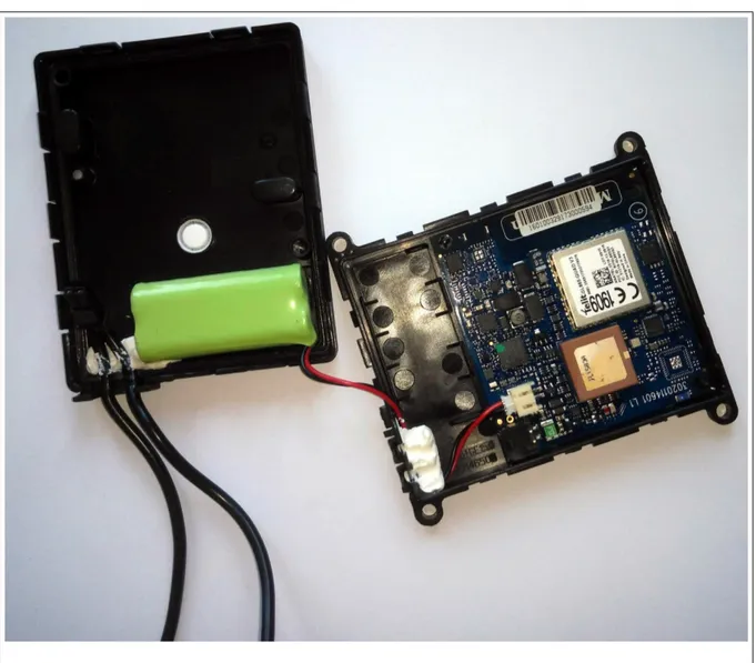
All these sensors can be bundled in a box, as in our case, and fitted on a vehicle. This box transmits data to a remote server using conventional cellular networks.

Figure 1.1: One of the sensor box used to collect data

(9)

phase where effectiveness of the program will be low, exclusively visually empiric, because of the need of rapid development and testing times. In a second and later phase, when quality of output will become more difficult to evaluate empirically, results will be compared to pictures and video footages captured in the data acquisition phases.

Aspiring software solution may face some challenges: sensor data gathering and transmission, correction of bad alignment, integration numerical error, precision reinforcement with multiple sensor fusion, representation of reconstructed trajectory.

Input date format is specified in a Physycom(PHYsics of COMplex SYstem) group’s Github online repository1.

I searched for an universal standard file format for inertial and GNSS data but I didn’t find previous work.

Briefly formats supported by the software are all the following combinations:

inertial inertial+GNSS

interpolated inertial fullinertial

non interpolated unmodified-inertial unmodified-fullinertial

The full-inertial format is the more complete one, containing both accelerometer, gyroscope and GNSS data. Indeed, the program will give a better output when provided with a full-inertial input file, as it has more data to improve reconstruction. Records can be interpolated, in this case have always data from all sensors, instead of only from one of them, as they can have different frequencies.

In the case input data isn’t interpolated, the software will take care of doing it.

The following table shows full-inertial data format in the order in which it is presented in the input files.

(10)

CHAPTER 1. INTRODUCTION Dataset Column Index Name Type Unit of measure Notes

0 Timestamp Float Seconds From 1/1/2000 UTC+1

1 Latitude Float Degrees From -90 to +90

2 Longitude Float Degrees From -180 to +180

3 Altitude Float Meters from sea level

4 Heading Float Degrees Measured from magnetic

north, from 0 to 360

5 Speed Float Km/h

6 Acceleration X Float g-unit Inertial

7 Acceleration Y Float g-unit Inertial

8 Acceleration Z Float g-unit Inertial

9 Angular speed X Float Degrees/Second right-handed

reference system

10 Angular speed Y Float Degrees/Second right-handed

reference system

11 Angular speed Z Float Degrees/Second right-handed

reference system

12 Acceleration module Float g-unit

13 Relative time Float Seconds From first record

I decided to visualize the reconstructed trajectory animated on the 3D modeling software Blender. The decision is motivated by the fact that Blender is a popular open source software and has an API to interact with. Additionally, it’s already used inside the research group and one of its member is a 3D-artist specialized on it.

Road vehicle crashes reconstruction has already been a case study, with both inertial and GNSS data, for example in the work of S. Tadic [10].

None of the work I found ever dealed with computational problems, neither provided a 3D visual-ization of the reconstruction.

This Thesis consists of 9 chapters: after this introduction, in chapter 2 we will look to some mathematical notions necessary to comprehends techniques used in the project, then in chapter 3 I will write about what programming language I decided to use and what libraries

The chapters that follow are a description of the principal code parts: error reduction, vehicle rotation, numerical integration and the Blender add-on. Then in chapter 6 I included a part about software engineering practice I followed during the development of this project.

Finally, there’s a conclusion chapter, with a recap of all the topics covered and a description of possible future improvements.

(11)

C

H A P T E R

2

M

ATHEMATICAL BACKGROUND

In this chapter I will introduce some mathematical and physics notion used in the project. The first part of the chapter deals with numerical integration, a technique used to computationally calculate the integral of physics quantities like acceleration and velocity to get the trajectory traveled by the vehicle. The second part deals with quaternion, a number system useful to handle rotations in tridimensional spaces, more efficient when dealing with multiple composition of rotations than rotation matrices.

2.1 Numerical integration

Records in input dataset may not be equally spaced, which means that if ti is a timestamp of a

record at position i, then ∃k,(tk− tk−1) 6= (tk+1− tk).

This implies that I can’t use Simpson integration method, because it’s a Newton-Cotes quadrature rule and it assumes that data points are equally spaced. [3]

Using a similar approach, interpolating with a second grade polynomial, I implemented an algorithm suitable for irregularly spaced data. [2]

Let’s considering these consecutive points (t1, y1), (t2, y2), (t3, y3) and a finite space of real functions,

with its base of representation_φ0,φ1, ...,φn. Each function of the space can be defined as a linear

combination of the basis:

φ(x) =

n

X

i=0

aiφ(x)

Let’s also consider the canonic form, where the basis are monomialφi= xi∀n_i=0

Indeed, every polynomial can be represented as a linear combination of monomials.

(12)

CHAPTER 2. MATHEMATICAL BACKGROUND

to pass through the points (ti, yi).

         at2₁+ bt1+ c = y1 at2₂_{+ bt}₂_{+ c = y}₂ at2₃_{+ bt}3+ c = y3     a b c         t2₁ t1 1 t2₂ t₂ 1 t2₃ t3 1    =     y1 y₂ y3         a b c    =     t2₁ t1 1 t2₂ t2 1 t2₃ t₃ 1     −1    y1 y2 y₃    

Once a, b, c are found the integral of the parabola can be calculated as: Z t3 t1 y(x)dx = Z t3 t1 ax2_{+ b y + cdx =} ·_a 3x 3 +b 2x 2 + cx ¸t3 t1 =a 3(t3− t1) 3 +b 2(t3− t1) 2 + c(t3− t1)

Unlike classic Simpson method, this allow us to calculate also half of the area bound by the parabola, simply evaluating integralRt2

t1 y(x) dx or Rt3 t2 y(x) dx instead of Rt3 t1 y(x) dx

2.2 Quaternions

Quaternions are an extension of complex numbers usually represented in the form: q = a + xi + y j + wk

where a, x, y, w are real numbers and i, j, k are called quaternion units. with the property (i jk) = −1

a is called scalar or real part of the quaternion, while x, y, w is the tridimensional vector or imaginary part. [6]

Quaternions have been formalized by the Irish mathematician William Hamilton in 1843. If the scalar part is equal to zero then the quaternion is called pure.

2.2.1 Vector rotations with quaternions

Given a point v ∈ R3, its rotation around versor x = {ax, ay, az}by an angleθcan be obtained in

the following way:

p0_{= q pq} where:

(13)

2.2. QUATERNIONS

• p is a pure quaternion with the vector part equal to v

• q is a quaternion representing rotation q = eθ2(axi+ayj+azk) = cos¡θ

2¢ +(axi + ayj + azk) sin

¡θ

2

¢

• q is the conjugation of quaternion q definied as q = (s,−v) = s − xi − y j − wk = e−θ2(axi+ayj+azk) = cos¡θ

2¢ − (axi + ayj + azk) sin

¡θ

2

¢

• p0 _{is a pure quaternion with its vector part equal to vector v rotated}

2.2.2 Product of quaternions

Given two quaternion q1 and q2defined as:

q1= (s1, v1) = s1+ a1i + b1j + c1k

q2= (s2, v2) = s2+ a2i + b2j + c2k

then their product can be defined as: q1q2= (s1s2− v1· v2, s1v2+ s2v1+ v1× v2)

2.2.3 Quaternion product isn’t commutative

q1q26= q2q1

is equivalent to

(s1s2− v1· v2, s1v2+ s2v1+ v1× v2)

6=

(s1s2− v1· v2, s1v2+ s2v1+ −(v1× v2))

by the anticommutative property of vector product [6] a × b = −(b × a)

2.2.4 Comparison with rotation matrices

Matrices can be used to perform rotation. [5] A quaternion can be associated with a rotation matrix and vice versa. [6]

Aside from memory usage, where quaternions are more efficient, the time complexity must take into account the conversion between rotation representations, as from axis-angle in our case, and actual context of usage as explained in the following.

Performance can be evaluated at a high-level by counting the number of operations needed to perform conversions and rotations. Operations like additions or subtractions, multiplications, divisions and trigonometric function like sines and cosines.

In the following analysis I will leave out performance optimization that computer systems can apply in some situations, like for example the simultaneous calculations of sine and cosine

(14)

CHAPTER 2. MATHEMATICAL BACKGROUND

performed by modern machine. Just looking at number of operations should give a general idea of difference between rotation representations.

Axis-angle to matrix conversion requires 13 additions, 15 multiplications and 2 trigonometric calls.

Axis-angle to quaternion conversion requires 4 multiplications and 2 trigonometric calls. Rotating a vector using a rotation matrix requires 5 additions and 9 multiplications.

Rotating a vector using a quaternion, optimizing considering its scalar part zero, requires 17 additions and and 24 multiplications.

So it results that rotation matrix are more efficient in rotating a vector, but the real advantage of quaternions are rotation compositions. Indeed, composing two quaternions require only 12 additions and 16 multiplications while matrices, would have required 18 additions and 27 multiplications.

What follows is a comparison analysis of the number of operations required to rotate n vectors by a cumulative n angles represented as axis-angle notation. Those abbreviations are used: A: Additions / subtractions, M : Multiplications, F: trigonometric Functions

• rotation matrices: ((13A + 15M + 2F) + (5A + 9M) + (18A + 27M))n = (36A + 51M + 2F)n • quaternions: ((4M + 2F) + (17A + 24M) + (12A + 16M))n = (29A + 44M + 2F)n

(15)

C

H A P T E R

3

P

ROGRAMMING LANGUAGE AND LIBRARY CHOICES

3.1 Python

For this project, the Python programming language was chosen. [9]

Python is increasingly being used by the scientific community for its large collection of packages. It allows to link normal Python code to C / C++ extension when performance optimization is critically important.

In addition, Blender only offer a Python API.

All benchmarks showed are based on standard Python implementation CPython.

3.2 Python scientific stack

• Numpy is a data structure library for n-dimensional arrays. Instead of creating an object for each integer like vanilla Python, with related garbage collector overhead, it handles array in contiguous memory space like C. Another big performance advantage is through vectorized operations, that permit to modify multiple array elements with a syntax like they were a single value. For example, ifarris an array of n elements, to multiply each element for the constant value 3, one doesn’t need to use a cycle that iterate on array, but can just writearr * 3. This is not just syntactic sugar, but it offers to the interpreter additional informations, like that the operation would be on all elements without interruption from side effects, implying a performance improvements thanks to of optimized cache usage. • Pandas is a package for data analysis. Its main data type is calledDataFrameand

repre-sents a two-dimensional dataset.DataFramecan be easily created fromcsvfiles, offering various methods. It is possible to complete a project like this only with pandas, as it uses

(16)

CHAPTER 3. PROGRAMMING LANGUAGE AND LIBRARY CHOICES

numpy underneath, but it offers a very expressive interface that needs a lot of logic beneath with a non negligible overhead. For this reason I reduced the Pandas usage and called it only when strictly necessary.

• Scipy offers many mathematical routines on top of numpy arrays. I used mainly trigono-metric functions like arctangent, cosine and sine. It has big precision constant for example for Pi and offers vectorized routines for cross and dot products.

• Matplotlib is the most used python plotting library, most of the other plotting libraries are based on it trying to abstract and elevate its complex interface. Nevertheless one can create very appealing charts also with low-level Matplotlib methods, especially it offers full customization.

3.3 Quaternion libraries

My Project initially started with numpy-quaternion [1] but then moved to pyquaternion [11] because of the following reason:

• moble/quaternion didn’t work on Windows1, as stated in the readme. This was a blocking issue because the 3D artist of the group was using a Windows workstation.

• pyquaternion has a better documentation and more high-level methods

On the downside, pyquaternion has performance disadvantages. As an example the following code using numpy-quaternion

from numpy_quaternion import quaternion as Quaternion quaternions = np . array (

[ np . exp ( Quaternion ( * np . asarray ( delta_theta ) ) / 2) for delta_theta in delta_thetas ] )

runs in 0.665 milliseconds

while the following code using pyquaternion from pyquaternion import Quaternion quaternions = np . array (

[ Quaternion . exp ( Quaternion ( v e c t o r = d e l t a _ t h e t a ) / 2 ) for d e l t a _ t h e t a in d e l t a _ t h e t a s ] )

(17)

C

H A P T E R

4

I

NPUT DATA CLEANING

Input data from sensors doesn’t represent real measurement of vehicle physics quantities. Instru-ments have a measuring error, each one with different possible reasons. This chapter deals with techniques used in the project to reduce that error, whether it was experimental or systematic.

4.1 Stationary time detection

Most of the solutions used to remove errors are based on the assumption of a vehicle state, in particular the stationary one.

This can’t be detected by a near zero acceleration along all axis because vehicle could be moving with constant speed. So integrated speed should be used, but integrating acceleration vectors that need corrections can bring next code logic to make mistakes as well as being a waste of time, because integration should be recalculated after having applied corrections.

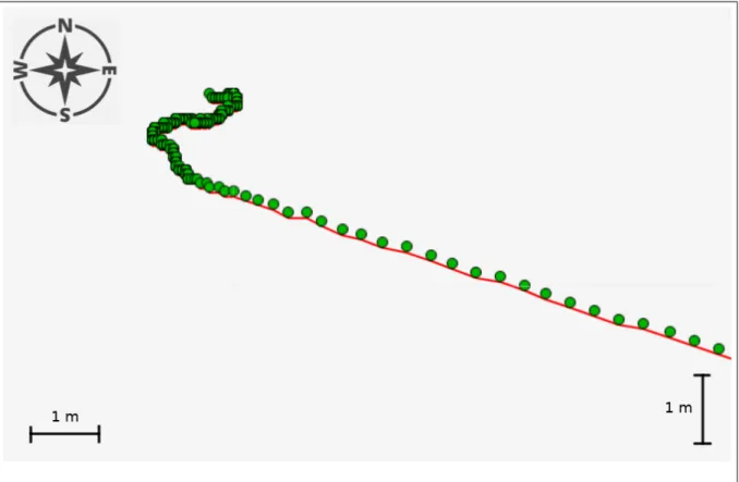
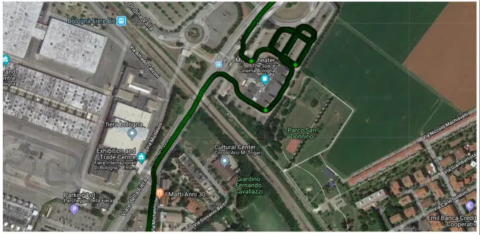
One solution can be to use non-directional speed from GNSS data by the measure device in the box. But this speed is under effect of Kalman filters to avoid measurement errors The filter is implemented directly inside box firmware, but reacts late to changes. One can differentiate numerically the GNSS positions to get a more precise speed and, on top of that, calculate stationary times. The choice of using speed subject to Kalman filters or the one derived should be based on GNSS sensor precision. Especially when vehicle is stopped, its error can be relevant as showed in the following picture.

(18)

CHAPTER 4. INPUT DATA CLEANING

Figure 4.1: Green points represent GNSS positions. On top-left GNSS error can be noticed in a situation where vehicle was stopped during experiment

To try to handle input data where vehicle never really stops, the algorithm for stationary time detection searches into dataset with an increasing threshold, until enough periods are found.

4.2 Gyroscope drift

Gyroscopes have a drift and an offset that is unavoidable. [4]

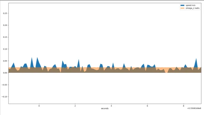
Offsets and their drifts can be measured when vehicles are stationary. Average value of angular velocities in stationary moments is an approximation of gyroscope offset. During motion, a gyro-scope exposed to heat increases its drift. So I made sure drift removal was applied continuously

(19)

4.3. NOISE REDUCTION

Figure 4.2: Data from stopped vehicle. Linear speed is near zero but gyroscope detects a non negligible angular speed

4.3 Noise reduction

Sensors are subject to noise both electronic (from the board itself or the electric supply) and mechanical (from their setup and the vehicle). In the data analyzed for this project I found spikes without any correlation to real events. There are various techniques to remove them, the one I used is the rolling average.

Given a series s, the centered rolling average with a window size w is defined as:

v_i₌ 1 w w 2 X j=0 v_j w X j=w2 v_j

where vi is the element of series s0, that is s with centered rolling average applied. The choice of

a value for window size is important. A value too small can lead to a noise left too high, while a windows size too large value can lead to flattening and reduction of measured value. For example with a value too high, an acceleration can be measured even before it actually started and overall highest value will be lower than in reality.

4.4 Correction of vertical alignment

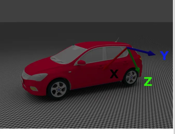
Box vertical unalignment is corrected by looking at gravitational acceleration on stationary times. Since g is always presented by the accelerometer, it can be used to determine vertical axis. This

(20)

CHAPTER 4. INPUT DATA CLEANING

technique only works assuming the vehicle rest on a flat surface.

Figure 4.3: Axes shows a sensor bad vertical alignment

Once obtained the rotation angle, the program rotates both local acceleration and angular velocities. After having done that, if in a following stationary time a bad vertical alignment is still found, the program prints a warning on the console to notify that the box become misaligned

(21)

4.5. CORRECTION OF HORIZONTAL ALIGNMENT

4.5 Correction of horizontal alignment

Box horizontal unalignment is corrected by looking for situations where ax> 0, ay> 0,ωz= 0. If

this state exists, then the car is sliding on ice without rotating on itself or there is an unalignment on the x y plane. The latter is more likely.

On unaligmnent, for example, an acceleration forward will be measured with both positive accelerations along x and y axis. Still in the situation described, the misalignment can be measured and corrected, still by rotating both local accelerations and angular velocities.

(22)

(23)

C

H A P T E R

5

R

OTATION WITH QUATERNIONS

This chapter deals with the usage of quaternions for rotations and in general with all of the project parts related to the transformation from a local frame of reference to a laboratory one.

5.1 From local to laboratory

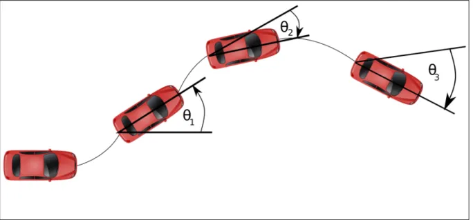
The program calculates the change of angular positions by integrating angular velocities, which are described in a local reference frame. This means that for calculating angular position at time t_i+1we must take into account angular position at time ti, so that it is reconstructed iteratively.

(24)

CHAPTER 5. ROTATION WITH QUATERNIONS

One of the first error I committed was to consider the rotation composition as the sum of angles on each axis. I was using the same integration routine used for linear dimensions, which performs the cumulative sum on each axis independently, i.e. the sum of the areas. When composing multiple rotations, for example when having a rotation around vertical versor ˆz by an angle

θz, besides addingθz to the vertical rotation, one must move rotation axes that belongs to the

horizontal x y plane.

So I divided the integration routine in two functions, one that returns an array of areas, the other that calls the first and then does the cumulative sum of the array of areas. I’ve done this also for keeping compatibility with others modules that were using the previous single function.

Then, once I had the angle variation vector 〈∆θx,∆θy,∆θz〉 the associated quaternions can be

created and multiplied together. Essentially, the two quaternion libraries I used in the project overload mathematical operators so compositions and rotations become more straightforward. For quaternion composition, initially I was using numpy.cumprod()[8] but this function was performing multiplications in reverse order, with respect to what I needed for my application. For example, callingcumprod()on a vector 〈a, b, c, d〉 will result in 〈a, ab, abc, abcd〉 while I needed 〈a, ba, cba, dcba〉

So I wrote some custom code to make quaternion composition, usingfunctools.reduce(), since it’s faster than using aforcycle.

quaternions = reduce ( lambda array , element : [ * array , element * array [ − 1 ] ] , quaternions ,

[ i n i t i a l _ q u a t e r n i o n ] )

The reason is that lambda use local scoped variables, that can be kept in register and cache, and that interpreter can preload next items.

5.2 World frame of reference

There exists an additional frame of reference, similar to the laboratory one described before but with an additional rotation in the horizontal plane. This frame of reference has y-axis oriented towards geographical north and x-axis to east. This is critically important for mixing GNSS data that is already in this frame of reference, with integrated inertial data.

To find the angle between GNSS positions and east, the program finds the first position that is at least 10 meters away from the initial one, then calculates the angle of this vector.

Assuming that the first motion of the vehicle is in the forward, direction given the previous calculated angle, all accelerations should be rotated.

(25)

5.2. WORLD FRAME OF REFERENCE

position with respect to the world frame of reference. Since the following angular positions are calculated from the first, no additional operations are needed, preventing the execution of O(n) operations, i.e. the rotation of all records.

(26)

(27)

C

H A P T E R

6

T

RAJECTORY INTEGRATION

Initially I coded both the square, the trapezoid and the parabola method, to analyze better suited my necessities. [3] The last one, from now on, will be called PaIS (Parabola integrator for Irregular Spaced data),

A quadrature formula of grade n provides the exact integral value of a polynomial of grade ≤ n, which means that it isn’t always necessary to use a formula with a high grade.

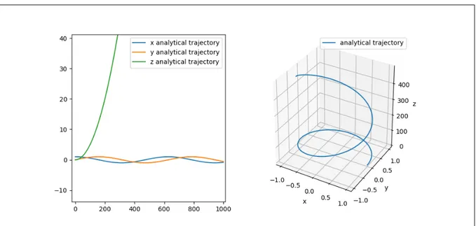
I verified experimentally the difference in error between integration methods by creating synthetic trajectories.

(28)

CHAPTER 6. TRAJECTORY INTEGRATION

then I compared the integrated one with the analytical.

Figure 6.2: Absolute error from analytical trajectory

Numpy offers a compact way to write operation even on large arrays. This is for example the trapezoid method in one line.

def t r a p z _ i n t e g r a t e _ d e l t a ( times , v e c t o r ) :

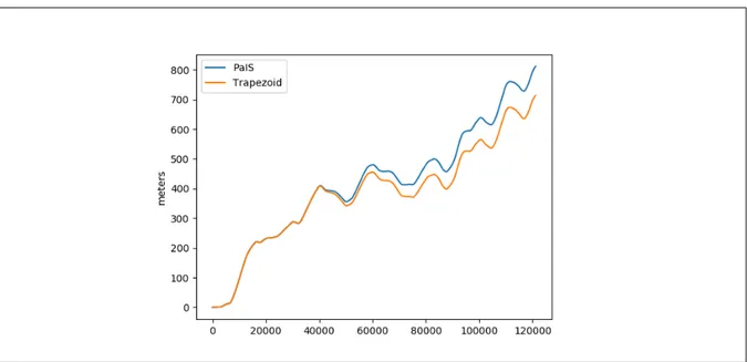
return ( ( ( v e c t o r [ : , : − 1 ] + v e c t o r [ : , 1 : ] ) * ( times [ 1 : ] − times [ : − 1 ] ) ) * 0 . 5 ) . cumsum ( ) Difference between PaIS and trapezoid can be seen after integrating for 40 thousands steps.

Figure 6.3: Difference between trapezoid and PaIS method on real world data

I decided to use the PaIS integrator because measures in discrete time produce a C0function,

(29)

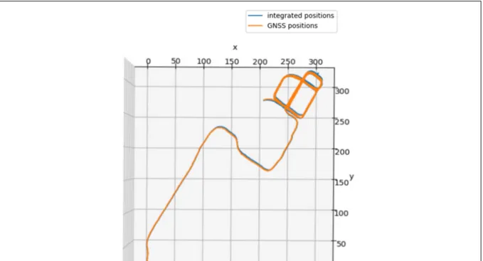
The errors were still too large, the integrated trajectory diverges after some time by moving away too much from the real trajectory. So I improved integrated trajectory using GNSS data, which is more precise but has lower frequency and has difficulties on finding orientation. In this way, the output trajectory benefits from both measures, using their respective advantages and reducing each other disadvantage. Accelerometer and gyroscope are really good in small time frames, but due to integrated quantities have precision problems on long time spans. On the other hand commercial GNSS sensors don’t have very precise positioning but they keep working steady for much times. I started from resetting the integrated position to the GNSS one every t times, but this was causing an edgy and irregular behavior that wasn’t realistic. I proceeded to implementing a contiguous weighted average, so that GNSS component is always present in the output trajectory but its impact is limited. Especially when GNSS signal is low,the position completely wrong, in the order of tens of meters. Giving a low weight to GNSS, like 1 on 99, avoid problems caused by low signals but still helps with correcting numerical integration error.

(30)

CHAPTER 6. TRAJECTORY INTEGRATION

Figure 6.5: The same path from data registered by sensors and elaborated by the program

(31)

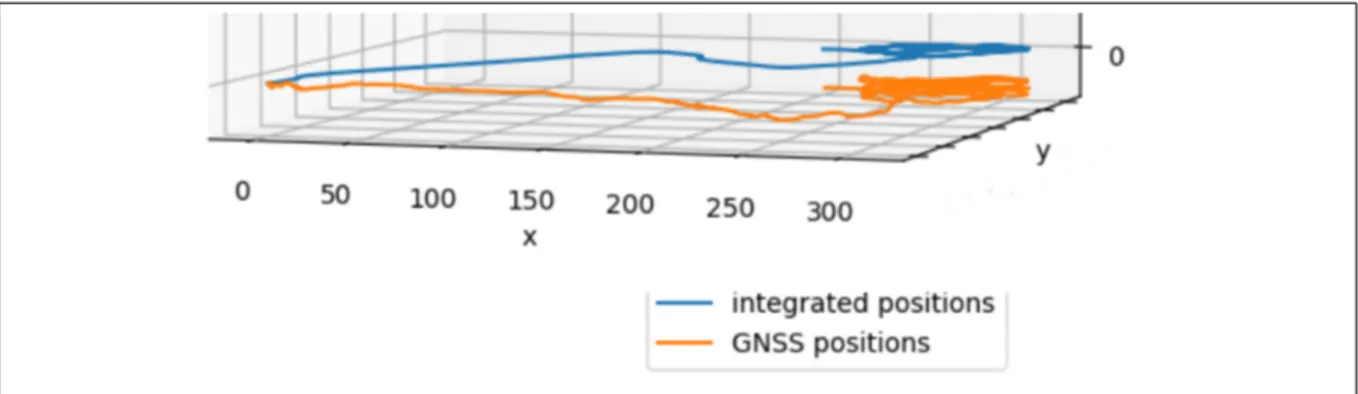
Figure 6.7: Note that GNSS and integrated path are distant on vertical axis. This is because altitude from GNSS system is extremely unreliable to determine vertical position. In my algorithm i Decided to neglect this information and only use the integrated accelerometer information.

(32)

(33)

C

H A P T E R

7

B

LENDER ADD

-

ON

Blender has a Python Application Programming Interface (API). Through the API, one can create a Python module and package it as Blender add-on. Add-ons are extension of Blender basic functionality, managed by a section of Blender settings and installable by file. As alternative to add-on to interact programmatically with Blender is possible to create a Python script and load it into the built-in text editor (and execute it) or give it as parameter while launching Blender from the command line. Add-ons provide versioning and authoring, remain activated between Blender files and don’t need to be loaded each time.

7.1 Blender API

All the operations are made throughbpyPython module.bpycan be subdivided additionally into:

• bpy.context: access to current active scene and elements.

• bpy.data: access to all objects in Blender document.

• bpy.types: built-in Python classes, usually extended.

• bpy.props: abstraction of a variable properties, having type bpy.types.*Property; if registered inbpy.props, it can be modified by graphical interface.

Frombpy.typesother classes used in the projects are:

• Operator: essentialy a function to manipulate objects. Every action that the user can do in Blender is coded like anOperator: like moving, modelling and sculpting objects.

(34)

CHAPTER 7. BLENDER ADD-ON

7.2 Blender add-on anatomy

An add-on can be a single Python file or a zip containing an__init__.pyfile and other comple-mentary files.

In both cases, the main Python file must have aregister()andunregister()function imple-mented.

Theunregister()takes care of callingbpy.utils.unregister_class(), for each class that needs to be loaded into Blender.

When loading a class, Blender performs sanity checks, making sure all required properties and functions are found, that properties have the correct type and that functions have the right number of arguments. register()function of registered class are called recursively and, for example,Panels are drawn on user interface at this moment.

Theunregister()have a totally opposite task compared toregister().

It should callbpy.utils.unregister_class()on every register call. It’s preferable to make the calls in the reverse order compared toregister().

Other objects defined in the Python add-on are:

• subclass ofPanelfor user-interface, a button to open a file system explorer dialog to select input dataset, an editable text field showing input dataset path and a button to launch dynamic reconstruction.

• StringPropertyfor storing input dataset file path and to share it between operators.

• subclasses ofOperatorfor reaction to buttons clicks on user interface and calling related project functions.

Finally, a Python dictionary calledbl_infois defined with add-on metadata as name, version and author. Those data are displayed in the list of add-ons in Blender settings.

7.3 Installation of dependencies

One particular challenge I faced was to have project library dependencies installed in blender internal interpreter.

There are three solution to this problem. Two solutions were discarded:

• Removing the Blender Python folder and Blender will fallback to system interpreter. But API supported Python version can be different to the system one and doing this is dangerous. • Changing Scripts path inside Blender setting, to look to another directory with a specific

structure. This directory must containsadd-ons, modulesandstartupdirectories. Project dependencies should be installed inmodulesdirectory. There are various problems to this

(35)

7.3. INSTALLATION OF DEPENDENCIES

of changing Scripts path, also it can be against the final Blender user will, requiring all previous installed add-ons to be moved to new directory.

The solution I decided to follow and implement is to increase Blender interpreter capabilities by installing the pip package manager on it and then using pip to install the dependencies listed in therequirements.txtfile. The whole process can be labeled as bootstrapping, as we start from a very small capability and we use it to have more at each step.

First step is to download a Python script which has pip binary included inside. To do this it is very useful theget-pip.pyscript. [7] Then,get-pip.pymust be run by the Blender interpreter so it will be linked to it.

In the Blender Python directory a pip executable will emerge so project dependencies can be installed with it and modules will be linked to.

Including the code to do this process in the add-on is crucial to have a singlezipto distribute and increase final user experience.

This part has been a bit tricky due to differences between operating system; both for file system structure and operating system interfaces to execute programs.

(36)

(37)

C

H A P T E R

8

S

OFTWARE ENGINEERING CONSIDERATION

This chapters deals with software engineering (SWE) topics: software design, quality measure and process management.

During SWE course I followed was focused on object oriented software design, that doesn’t really fit for this project. The domain doesn’t contain many objects to model and python classes introduce an overhead which is incompatible with performance required, taking into account input dimensions.

Anyway, even if I used a more functional approach, I still divided the codebase into modules using responsibility-driven design.

8.1 Requirements

After several discussions with my supervisor, I modeled the following functional requirements: 1. the software will support inputs in the format specified in the introduction chapter; 2. the software will use Blender API to animate a vehicle so that its linear and angular

positions reflect the one from which the input data is measured; Non functional requirements are:

1. performance: the software must at least elaborate a dataset of 100.000 records in less than five minutes;

2. user experience: the software must be easy to use also from a 3D artist point of view; 3. operating systems. the software must support of Windows and GNU/Linux ;

(38)

CHAPTER 8. SOFTWARE ENGINEERING CONSIDERATION

8.2 Structure

Satisfying functional requirement 1 is the main challenge of the project. Recreating a perfect reconstruction is very hard and requires many techniques as showed in the previous chapter. Following the methods previously illustrated the responsibilities of the software are:

1. input loading;

2. input parsing;

3. input format auto-detection;

4. noise reduction;

5. gyroscope offset drift reduction;

6. correction of vertical bad alignment;

7. correction of vertical bad alignment;

8. derivation of GNSS speed and acceleration;

9. moving from local to laboratory reference frame;

10. moving from laboratory to world reference frame;

11. integrate accelerations;

12. integrate velocities;

13. timestamps normalization;

14. dependencies auto-installation;

(39)

8.3. DEPENDENCY MANAGEMENT

Figure 8.1: UML diagram showing project modules and their dependencies. The numbers nears each modules states responsabilities assigned to it.

8.3 Dependency management

Current software development practices suggest to don’t reinvent the wheel and re-use as much as existing software as possible. Project stability is related to its dependencies’ stability. Delegating responsibilities to other trusted programmers reduce project risks and increase overall quality. Specifying explicitly project dependencies is useful both for the programmer and for the user, in particular specifying which version of each dependency the software is assured to work. Python has various tools to handle this, the most popular are pip+virtualenv and Conda.

Virtual environments allow to isolate Python packages on which the project depends on from the global system ones. This allows to use different packages version.

Pip (Pip Install Packages) can install packages from a the PyPi repository, the largest one containing more than 143 hundred packages, parsing a list file containting dependencies. Conda is a package manager designed for every language, instead virtualenv is only for Python. It was created from the PyData community to overcome Pip limitations and doesn’t use only

(40)

CHAPTER 8. SOFTWARE ENGINEERING CONSIDERATION

PyPi to retrieve packages. Instead it has customized version of python scientific packages like numpy, scipy and pandas, optimized for performance as Conda can work on a lower-level in target machine.

Initially, I was using Conda and I noticed a better performance, but when I created the Blender add-on code part that auto install dependencies I had to move back to virtualenv+pip because it was easier to install.

8.4 Unit testing

On the project I applied the principles of unit testing. I tried to create a test for every function I’ve written, sometimes even before the code itself to be tested, to make it minimal.

During this process I prepared a tool to produce syntetich trajectories, to overcome specific requirements of some tests. The tests I’ve written are incremental, some verify only small func-tionalities, others verify more overall features that use the small functionalities underneath. For example, I created a test with a complex trajectory similar to the one of a spring, to test integrator precision, then I created a circular trajectory, where body also rotate like a car in a roundabout to test, angular position integration and body rotation. In this way it is easier when a breaking change is introduced to debug and fix the problem.

Right now the test coverage, which is the percentage of code lines that are executed by automatic tests, of project’s principal modules is 86%.

(41)

C

H A P T E R

9

C

ONCLUSIONS

Thus thesis presented a software to reconstruct vehicle dynamics from inertial and GNSS data. I developed an algorithm to integrate physical quantities with a technique suitable also for not equally time separated records. Both acceleration and angular velocity are integrated; angular position is composed using quaternion performance advantages. Trajectory obtained from accelerometer and gyroscope is improved additionally by GNSS data, leading to a more precise and smooth path. The project has been implemented in Python, mainly take advantage of Numpy and Pyquaternion libraries functionalities. I created a standalone Blender add-on which auto-installs its dependencies and offers a graphical interface. Most of the code has been checked with automated testing.

9.1 Future Development

Several improvements can be implemented in following releases:

• the angular position reconstruction can still be improved significantly using some inference techniques (fusing data from other sensors, refining the analytical model of the dynamics) and also it tends to drift away due to numerical error. Cross-validating vehicle angular positions with accelerometer and GNSS can provide a better assessment on the error it has been accumulated and that must be corrected. Moreover, online maps API can be used to have an approximation of road slope;

• gyroscope offset can be additionally analyzed through unused data coming from the tem-perature sensor. In fact, it is well known that this erroneous behavior is strongly correlated with the sensor’s thermal state;

(42)

CHAPTER 9. CONCLUSIONS

• vertical positioning can be strongly improved by using barometer;

• data from sensors installed on different positions in the same vehicle can be merged, at the beginning using their known relative positions, and later even by self-calculating them; • usage of approximation instead of interpolation for GNSS precise positioning can be used

to reduce error when vehicle is in a stationary regime;

• to improve integration algorithm stability it is possible to explore different change of basis of second grade polynomial used;

• implementation of symplectic integration schemes which, due to their non-dispersive nature, can help improving the reconstruction;

• implementation of a new file format, based on HDF, to drastically improve I/O performances • parallelize execution, expecially in delta integration routine where it can be distributed on

(43)

R

INGRAZIAMENTI

Vorrei ringraziare tutto il gruppo di Fisica dei Sistemi Complessi, in specifico Stefano Sinigardi, Alessandro Fabbri, Nico Curti e Raffaele Pepe per il supporto e per il bel ambiente lavorativo in cui sono stato.

Vorrei ringraziare la mia famiglia per l’aiuto che mi hanno dato e perché mi hanno permesso di studiare seguendo le mie passioni.

(44)

(45)