Symbolic versus sub-symbolic approaches: a case study on training Deep Networks to play Nine Men’s Morris game

(1)

ALMA MATER STUDIORUM – UNIVERSITA’ DI BOLOGNA

SCUOLA DI INGEGNERIA E ARCHITETTURA

DIPARTIMENTO DISI

Corso di Laurea in INGEGNERIA INFORMATICA MAGISTRALE

TESI DI LAUREA in

FONDAMENTI DI INTELLIGENZA ARTIFICIALE M

Symbolic versus sub-symbolic approaches: a case study on training Deep Networks to play Nine Men’s Morris game

CANDIDATO RELATORE:

Galassi Andrea Chiar.ma Prof.ssa Mello Paola

CORRELATORI Ing. Chesani Federico Dott. Lippi Marco

Anno Accademico 2015/2016 Sessione III

(2)

(3)

“The answer that came to me again and again was play. Every human society in recorded history has games.

We don't just solve problems out of necessity. We do it for fun.

Even as adults.

Leave a human being alone with a knotted rope and they will unravel it.

Leave a human being alone with blocks and they will build something. Games are part of what makes us human.

We see the world as a mystery, a puzzle,

because we've always been a species of problem-solvers.” -

(4)

(5)

5.2 Networks architecture ... 44 Residual network ... 45 Dense network ... 46 Feed-forward network ... 46 5.3 Dataset ... 47 Dataset creation ... 47 Dataset composition ... 48 5.4 Networks Training ... 50 5.5 Play mode ... 51 Legality check ... 52 5.6 Implementation ... 52 Data Processing ... 53 Legality ... 53

(7)

6 Experimental Results ... 55

6.1 Tuning on restricted dataset ... 55

FFNets testing ... 55

ResNets testing ... 58

Comparison between the architectures ... 60

6.2 Tuning on whole dataset ... 61

TO network tuning ... 62

FROM network tuning ... 64

REMOVE network tuning ... 65

Best Networks performance ... 67

6.3 Accuracy test ... 68

6.4 Legality test ... 70

6.5 Gaming test ... 71

7 Conclusions and future developments ... 74

7.1 NNMM and its neural networks ... 74

7.2 Symbolic and sub-symbolic systems ... 75

Bibliography ... 77

(8)

List of Figures and Tables

FIGURE 3.1REPRESENTATION OF NINE MEN’S MORRIS GAME BOARD ... 11

FIGURE 3.2SYMMETRIES IN NINE MEN’S MORRIS GAME BOARD ... 13

FIGURE 3.3ENUMERATION OF NINE MEN’S MORRIS BOARD POSITIONS ... 14

FIGURE 3.42D REPRESENTATION OF NINE MEN’S MORRIS BOARD (LEFT) AND RELATIONSHIP WITH THE BOARD (RIGHT).THE WHITE CELLS CONTAINS RELEVANT ELEMENTS. ... 14

FIGURE 3.53D REPRESENTATION OF THE BOARD STATE.THE THREE COLORS, YELLOW, ORANGE AND RED, DIFFERENTIATE THE ELEMENTS BELONGING RESPECTIVELY TO THE INNER, THE MIDDLE AND THE OUTER SQUARE OF THE BOARD.THE GREY ELEMENTS ARE NOT RELEVANT. ... 15

FIGURE 3.6DIFFERENCES BETWEEN LOGICAL DISTANCE (IN BLUE) AND “PHYSICAL” DISTANCE (IN RED) IN THE 2D REPRESENTATION (LEFT) AND THE 3D REPRESENTATION (RIGHT) OF THE BOARD ... 16

FIGURE 3.7EXAMPLE OF GAME STATE IN INTERNATIONAL DRAUGHTS ... 18

FIGURE 3.8EXAMPLE OF GAME STATE IN CHESS ... 19

FIGURE 3.9INITIAL GAME STATE IN OTHELLO ... 21

FIGURE 3.10EXAMPLE GAME STATE IN GO ... 22

FIGURE 4.1SIMPLIFIED MODELS OF BIOLOGICAL NEURON AND ARTIFICIAL NEURON.THE BIOLOGICAL NEURON GATHER IMPULSES/INPUTS THROUGH DENDRITES, AGGREGATES THEM IN THE SOMA AND PROPAGATE THE IMPULSE/OUTPUT WITH THE AXON ... 24

FIGURE 4.2SIGMOID FUNCTION PLOTTING ... 25

FIGURE 4.3FEED-FORWARD NEURAL NETWORK ARCHITECTURE SCHEME ... 26

FIGURE 4.4RECTIFIER FUNCTION PLOTTING ... 33

FIGURE 4.5IN A RELU NETWORK THE INPUT OPERATES A PATHS SELECTION ... 33

FIGURE 4.6EXAMPLE OF A NETWORK BEFORE (LEFT) AND AFTER (RIGHT) DROPOUT APPLICATION [37]... 34

FIGURE 4.7A BUILDING BLOCK OF A RESIDUAL NETWORK ... 37

FIGURE 4.8THREE DIFFERENT VERSIONS OF RESIDUAL NETWORKS BUILDING BLOCKS ... 37

FIGURE 4.9AN EXAMPLE OF DENSE NETWORK MADE BY TWO DENSE BLOCKS (ON THE LEFT), AN EXAMPLE OF DENSE BLOCK MADE BY TWO LAYERS (IN THE MIDDLE) AND THE DETAILED COMPOSITION OF A SINGLE CONVOLUTIONAL LAYER (ON THE RIGHT) ... 38

TABLE 5.1BINARY RAW REPRESENTATION OF THE INPUT ... 44

TABLE 5.2INTEGER RAW REPRESENTATION OF THE INPUT ... 44

FIGURE 5.1AN EXAMPLE OF A RESIDUAL NETWORK WITH TWO BLOCKS AS IMPLEMENTED IN THE SYSTEM, WITH A FOCUS ON THE SINGLE BUILDING BLOCK (ON THE RIGHT) ... 45

FIGURE 5.2AN EXAMPLE OF DENSE NETWORK AS IMPLEMENTED (LEFT), WITH A FOCUS ON AN EXAMPLE DENSE BLOCK MADE BY TWO LAYERS (MIDDLE) AND A FOCUS ON THE COMPOSITION OF A SINGLE FULLY-CONNECTED LAYER (RIGHT) ... 46

FIGURE 5.3TWO EXAMPLE OF DATASET ENTRIES AND THEIR CORRESPONDING MEANING AS A GAME STATE AND A MOVE (IN GREEN).THE PLAYER’S STONES ARE COLOURED IN BLUE, WHILE ITS ADVERSARY’S STONES ARE COLOURED IN RED. ... 49

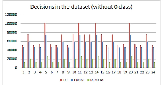
FIGURE 5.4DISTRIBUTION OF THE DECISIONS IN THE EXPANDED DATASET AMONG THE DIFFERENT CLASSES, WITHOUT CONSIDERING THE 0 CLASS ... 49

FIGURE 5.5COMPOSITION OF THE EXPANDED DATASET AMONG THE DIFFERENT PHASES OF THE GAME ... 50

(9)

FIGURE 5.6SYSTEM GAMING MODE WORKFLOW ... 52

TABLE 6.1CONFIGURATION OF FFNETS TRAININGS ON PARTIAL DATASET FOR DROPOUT TESTING... 56

FIGURE 6.1VALIDATION ERROR FOR DIFFERENT PERCENTAGES OF INPUT DROPOUT IN FFNETS ... 56

FIGURE 6.2VALIDATION ACCURACY FOR DIFFERENT PERCENTAGES OF INPUT DROPOUT IN FFNETS ... 56

TABLE 6.2CONFIGURATION OF FFNETS TRAININGS ON PARTIAL DATASET FOR LAYERS WIDTH TESTING ... 57

FIGURE 6.3VALIDATION ERROR FOR DIFFERENT NUMBER OF NEURONS IN FFNETS ... 57

FIGURE 6.4VALIDATION ACCURACY FOR DIFFERENT NUMBER OF NEURONS IN FFNETS ... 57

TABLE 6.3CONFIGURATION OF RESNETS TRAININGS ON PARTIAL DATASET FOR DROPOUT TESTING... 58

FIGURE 6.5VALIDATION ERROR FOR DIFFERENT PERCENTAGES OF DROPOUT IN RESNETS .. 58

FIGURE 6.6VALIDATION ACCURACY FOR DIFFERENT PERCENTAGES OF DROPOUT IN RESNETS ... 58

TABLE 6.4CONFIGURATION OF FFNETS TRAININGS ON PARTIAL DATASET FOR DEPTH TESTING... 59

FIGURE 6.7VALIDATION ERROR FOR DIFFERENT NUMBER OF RESIDUAL BLOCKS IN RESNETS ... 59

FIGURE 6.8VALIDATION ACCURACY FOR DIFFERENT NUMBER OF RESIDUAL BLOCKS IN RESNETS ... 59

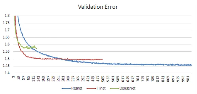
FIGURE 6.9VALIDATION ERROR FOR THE BEST TO NETWORK FOR OF EACH ARCHITECTURE60 FIGURE 6.10VALIDATION ACCURACY FOR THE BEST TO NETWORK FOR EACH ARCHITECTURE ... 60

TABLE 6.5CONFIGURATION OF THE BEST RESNET TRAINING ON THE PARTIAL DATASET .... 61

TABLE 6.6CONFIGURATION OF THE BEST FFNET TRAINING ON THE PARTIAL DATASET ... 61

TABLE 6.7CONFIGURATION OF THE BEST DENSENET TRAINING ON THE PARTIAL DATASET 61 TABLE 6.8CONFIGURATIONS OF TO TRAININGS OF THE NETWORKS ON WHOLE DATASET ... 62

FIGURE 6.11VALIDATION ERROR FOR THE TO NETWORKS ... 63

FIGURE 6.12VALIDATION ACCURACY FOR THE TO NETWORKS ... 63

FIGURE 6.13TIME NEEDED TO REACH THE BEST ACCURACY FOR THE TO NETWORKS ... 63

TABLE 6.9CONFIGURATIONS OF FROM TRAININGS OF THE NETWORKS ON WHOLE DATASET ... 64

FIGURE 6.14VALIDATION ERROR FOR THE FROM NETWORKS ... 64

FIGURE 6.15VALIDATION ACCURACY FOR THE FROM NETWORKS ... 65

FIGURE 6.16TIME NEEDED TO REACH THE BEST ACCURACY FOR THE FROM NETWORKS ... 65

TABLE 6.10CONFIGURATIONS OF REMOVE TRAININGS OF THE NETWORKS ON WHOLE DATASET ... 66

FIGURE 6.17VALIDATION ACCURACY FOR THE REMOVE NETWORKS ... 66

FIGURE 6.18VALIDATION ACCURACY FOR THE REMOVE NETWORKS ... 67

FIGURE 6.19TIME NEEDED TO REACH THE BEST ACCURACY FOR THE REMOVE NETWORKS ... 67

FIGURE 6.20ACCURACY OF THE BEST NETWORKS AT THE END OF THE TEST TRAINING ... 68

FIGURE 6.21ACCURACY OF NNMM IN THE DIFFERENT DECISIONS ... 69

FIGURE 6.22ACCURACY OF THE BEST NETWORKS AT THE END OF THE GAME TRAINING ... 71

TABLE 6.11OUTCOMES OF THE MATCHES PLAYED BY DM AND NNMM AGAINST OTHER AI ... 72

(10)

(11)

Abstract

In the last few years, due to the new Deep Learning techniques, artificial neural networks have completely revolutionized the technologic landscape, demonstrating themselves effective in many tasks of Artificial Intelligence and similar research fields. Therefore it could be interesting to analyse how and by what measure deep networks can replace symbolic AI systems. After the impressive results obtained in the game of Go, the game of Nine Men’s Morris has been chosen as case of study in this work, because it is a widely spread and deeply studied board game. Therefore, the Neural Nine Men’s Morris system has been created, a completely sub-symbolic program which uses three deep networks to choose the best move for the game. Networks have been trained over a dataset of more than 1,500,000 pairs (game state, best move), created according to the choices of a symbolic AI system. The tests have demonstrated that the system has learnt the rules of the game, predicting a legal move in more than 99% of the cases. Moreover, it has reached an accuracy on the dataset of 39% and has developed its own game strategy, which results to be different from its trainer one, proving itself to be a better or a worse player according to its adversary. Results achieved in this case study show that the key issue in designing state-of-the-art AI systems in this context seems to be a good balance between symbolic and sub-symbolic techniques, giving more relevance to the latter, with the aim to reach a perfect integration of these technologies.

Le reti neurali artificiali, grazie alle nuove tecniche di Deep Learning, hanno completamente rivoluzionato il panorama tecnologico degli ultimi anni, dimostrandosi efficaci in svariati compiti di Intelligenza Artificiale e ambiti affini. Sarebbe quindi interessante analizzare in che modo e in quale misura le deep network possano sostituire le IA simboliche. Dopo gli impressionanti risultati ottenuti nel gioco del Go, come caso di studio è stato scelto il gioco del Mulino, un gioco da tavolo largamente diffuso e ampiamente studiato. È stato quindi creato il sistema completamente sub-simbolico Neural Nine Men’s Morris, che sfrutta tre reti neurali per scegliere la mossa migliore. Le reti sono state addestrate su un dataset di più di 1.500.000 coppie (stato del gioco, mossa migliore), creato in base alle scelte di una IA simbolica. Il sistema ha dimostrato di aver imparato le regole del gioco proponendo una mossa valida in più del 99% dei casi di test. Inoltre ha raggiunto un’accuratezza del 39% rispetto al dataset e ha sviluppato una propria strategia di gioco diversa da quella della IA addestratrice, dimostrandosi un giocatore peggiore o migliore a seconda dell’avversario. I risultati ottenuti in questo caso di studio mostrano che, in questo contesto, la chiave del successo nella progettazione di sistemi AI allo stato dell’arte sembra essere un buon bilanciamento tra tecniche simboliche e sub-simboliche, dando più rilevanza a queste ultime, con lo scopo di raggiungere la perfetta integrazione di queste tecnologie.

(12)

Chapter 1

1 Introduction

Artificial neural networks first appeared more than 60 years ago and in the last decade have once again improved artificial intelligence researches and applications, achieving impressive results in tasks such as image and speech recognition and classification, natural language processing, sentiment analysis, and game playing.

The new deep learning techniques take advantage from a huge amount of unstructured data and knowledge and the impressive computational power of modern computer architectures in order to define very fast and effective machine learning algorithms, considered very interesting and promising by all the major ICT companies that are currently investing on them [1].

As evolution of neural networks, deep learning technologies are sub-symbolic techniques that does not require an explicit representation and modelling of the problem to be solved. The solution is “hidden” inside the configuration of the networks and in the weights of its connections. On the other hand, symbolic systems, in which knowledge and reasoning are expressed through rules and symbols manipulation, are still used in several Artificial Intelligence applications since they are generally more reliable, transparent and seem to perform better when solving problems where knowledge is explicit and specialized.

Nowadays, a very important research issue in the Artificial Intelligence area is trying to exploit the advantages of both symbolic and sub-symbolic approaches, combining or integrating them in a single hybrid system, therefore solving their apparent dichotomy.

If we consider the context of board games, traditionally, Artificial Intelligence researchers have used symbolic techniques to approach the challenge to play, obtaining the impressive result of defeating human champions in many classical games like Chess, Draughts or Othello. Combining symbolic systems and neural networks, relying on the latter for tasks such as the evaluation of game states, the new hybrid systems have demonstrated themselves better player than their “ancestors”, being able to triumph even in the game of Go. Recognized as one of the most difficult

(13)

board game existing, until the last year the game of Go was considered too difficult for an AI system, but the hybrid program AlphaGo proved this belief wrong, earning itself the title of first computer program to defeat a Go international champion.

A spontaneous question which rises is if a sub-symbolic system could substitute entirely a symbolic one. In particular, in the context of board games, the system should learn the game rules and constraints and optimizing some objective, providing a solution which is both good and acceptable without any a priori explicit knowledge about the problem and without any human intervention. If this is the case, what are the strengths and weaknesses of this approach with respect to a symbolic one and how could them be merged together in a synergic way?

The purpose of this thesis is to investigate this issue and try to give a first answer to this question by using a case study and therefore by designing, implementing testing a pure sub-symbolic system able to play a popular board game, Nine Men’s Morris, which is wide-spread, deeply studied and solved.

The product of this work is Neural Nine Men’s Morris (NNMM), a program able to play the game following its rules and taking smart decisions using only sub-symbolic machine learning techniques based on neural networks. To train it, a dataset of 1,628,673 “good moves” has been created, which contains a set of states and the corresponding best moves according to a symbolic AI, that has the role of “teacher” of NNMM.

What is aimed to achieve is not a symbolic AI system that chooses the best move according to explicit rules and heuristics by considering future, possible moves (states) that it and its adversary will make and therefore trying to identify the more promising move that would lead to win the game (goal state). The NNMM system is sub-symbolic instead and will learn to play simply following its “instinct”, developed after considering a huge number of examples, rather than following, a priori, a complex strategy which explicitly involves knowledge elicited from human expert player about the game.

Using supervised learning and neural networks, the desired system will independently learn to recognize some patterns and features and to associate them to a particular move, so it will be able to predict the best move simply by watching the board. Furthermore, fed with thousands possible moves, this system will understand when a move is considered legal, even though nobody has explained it the rules of the game.

(14)

To make a comparison, the system will not be like a person who learns to play reading the rule book or strategy guides, but simply watching an expert playing.

To verify if these goals have been accomplished, Neural Nine Men’s Morris will be tested firstly confronting its choices with the dataset ones and verifying if it respects the game rules, than its skill as player will be tested playing against other AI, among which there will be its “teacher”.

Chapter 2 presents the problems of representing knowledge and how a system can increase its knowledge, describing the main approaches and the different types of learning.

Chapter 3 examines the game of Nine Men’s Morris, analysing its rules, the way it can be represented in a computer system and comparing it to other popular board games.

Chapter 4 explains neural network models, showing some architectures invented through the decades and illustrating the principles behind them, finally focusing on approaches that have been proved successful playing board games.

Chapter 5 describes what has been the approach to the problem, the dataset that has been created, the system which has been designed, its neural networks and how they have been realized and trained.

Chapter 6 concerns the tests that have been done to tune the networks and evaluate the system in terms of accuracy with respect to the dataset, respect of game rules and skill as player against other AI.

Chapter 7 sums up what tests have proven and proposes possible future works on this subject, both as improvements to NNMM and further studies on the sub-symbolic systems.

(15)

Chapter 2

2 Knowledge and learning

Artificial intelligence is probably one of the computer science research fields that deals the most with philosophy or cognitive science. Apparently vague and abstract questions like “what is knowledge?” and “what means to learn” became fundamental, because they are strictly linked with very practical questions that researches deal with:

 How can knowledge be represented?

 How can a system be taught with new knowledge?

Knowledge representation and machine learning are considered two fundamental aspects for an AI that has the ambition to pass the Touring Test: it must store what it knows, it must adapt to new circumstances and be able to extrapolate patterns [2].

2.1 Symbolic approaches

The theory that human thinking is a kind of symbols manipulation and that can be expressed as formal rules is deeply-rooted in western philosophy and expressed partially by Hobbes, Leibniz, Hume and Kant [3]. Therefore, for long time the dominant theory has been that many aspects of intelligence could be achieved manipulating symbols, so the best way to represent knowledge could be only to use symbols.

This position is well embodied in Simon and Newell physical symbol system hypothesis:

“A physical symbol system has the necessary and sufficient means for general intelligent action” [4]

Following this idea, what are called physical symbol systems (or formal systems) have been defined and realized: systems which use physical patterns called symbols, combine them into structures called expressions and manipulate them with processes to obtain new expressions.

(16)

Examples of symbolic systems are formal logic, algebra or the rules of a board game such as chess: the pieces are the symbols, the positions of the pieces on the boards are the expressions and the legal moves that modify those positions are the processes.

An important idea linked to this approach is the search space [5]. It is supposed that in any problem there is a space of states, defined by an initial state, a set of actions that can be done and a transition model that defines the consequences of the actions. Therefore the state space forms a direct graph in which the nodes are the states and the links are the actions. The solution to a problem is the sequence of actions that determine the path from the initial state to a goal state. Considering that a solution must begin from the initial state, the possible actions sequences form a search tree which has the initial state as root. Having a test that allows to determine if a given state is a goal state, an intelligent system can navigate the tree with the aim of founding a goal state and therefore the solution. To speed up the process, knowledge can be provided to the search algorithm, allowing it to evaluate the states and to infer faster a path to the goal [2].

Symbolic approaches are still researched today and have produced one of the first truly successful forms of artificial intelligence: expert systems. Built mainly by if-then rules, they are designed to solve complex problems and imitate the decision-making ability of human expert. They are knowledge-based system, which means that are made by two distinct part: a knowledge base that represent facts about the world and an inference engine that permit them to discover new knowledge basing on the one that is already possessed.

2.2 Sub-symbolic approaches

Physical symbol system hypothesis has been criticized under many aspects because, according to some researchers, does not resemble a human intelligence.

According to Dreyfus, part of the human intelligence derive from unconscious instincts that allow people to take quick decision using intuition; this aspect is unlikely to be captured by a formal rule [6].

The theory of embodied cognition affirms that symbol manipulation is just a little part of human intelligence, most of it depends by unconscious skills that derives from the body rather than the mind.

(17)

Brooks has written that sometimes symbols are not necessary: in the case of human basic skills like motion or perception they are a complicated representation of something that is far more simple [7].

The poor results obtained with symbol manipulation models, especially in their inability to handle flexible and robust processing in an efficient manner, lead in the 1980 to the connectionist paradigm [5]. It does not deny that at some levels human beings manipulate symbols, but suggest that this manipulation is not implied in cognition; it tries to model the source of all this unconscious skills and instinct as an interconnected network of simple and almost uniform units [2]. After an initial period of enthusiasm, the interest in connectionist models and systems had lowered for several years, but has rose again recently, stimulated by the great results achieved by the combination of new models and modern hardware.

Even though connectionist and symbolic approaches are viewed as complementary, not competing, it is very interesting to investigate their limits comparing their results on the same task.

2.3 Learning

“An agent is learning if it improves his performance on future tasks after making observations about the world. Learning

can range from the trivial, as exhibited by jotting down a phone number, to the profound, as exhibited by Albert Einstein, who inferred a new theory of the universe” [2]

The purpose of machine learning is to give to a system the ability of make predictions about unknown data, predictions that will be helpful for the users or for the system itself, letting it able to improve its performance on a task. Taking advantage of a base knowledge acquired during training, the system infers new knowledge in the form of a model of the data and behaves according to it, letting the system able to perform tasks for which it has not explicitly programmed for.

Indeed, there are many scenarios in which the system cannot be programmed for all the possible situations in which it will have to act, so it is fundamental that it could take decisions by its own experience. For example, the number of possible configurations it could be too vast for being anticipated by the designer, or in a dynamic environment could be impossible to predict which

(18)

changes my occur during time or simply human programmers could have no idea how to program a solution [2].

Training can be divided into three categories according to the feedback that is provided to the system: unsupervised learning, reinforcement learning and supervised learning,

In unsupervised learning, the system analyse a set of known inputs and learns patterns that characterize the domain; a typical task is detecting potentially useful clusters of input example, which is called clustering.

Reinforcement learning aim to teach a system to take action in a variable environment; depending on how much the system output is appropriate to the environment state, the system is fed with a series reinforcements which can be rewards or punishments.

Supervised learning consists into giving to the system a set of couple of inputs and desired output, making it learn the relation between input and output.

In this work, to train the neural networks will be used supervised learning techniques, therefore it is necessary to describe this category in more detail.

Supervised Learning

Formally, the task of supervised learning is [2]:

Given a training set of N example input-output pairs (𝑥₁, 𝑦₁), (𝑥₂, 𝑦₂), … (𝑥_𝑁, 𝑦_𝑁)

where each 𝑦_𝑗 has been generated by an unknown function 𝑦 = 𝑓(𝑥)

discover a function ℎ that approximates the true function 𝑓

Function ℎ is called hypothesis and learning means to search through the space of all the possible hypothesis for one that is consistent and generalize well.

A consistent hypothesis is an hypothesis which agrees with training data and it is said that generalizes well if it is able to predict the correct output for inputs which has not be trained on; this can be verified using only a part of the available data for the training set and using the remaining part as a test set.

(19)

According to the number of times that an hypothesis makes a correct or an incorrect prediction, there are several ways to measure its goodness. Given an hypothesis ℎ, a couple (𝑥, 𝑦) and calling a prediction ℎ(𝑥) wrong if 𝑦 ≠ ℎ(𝑥), correct otherwise, it is possible to define the error rate of ℎ as the proportion between the number of wrong predictions and the number of total predictions, in the same way is possible to define the accuracy of ℎ as the proportion between the number of correct predictions and the number of total predictions.

These measures could be not informative enough, because not all the wrong prediction could be equally negative: for example, in a mail system, could be better to label a spam mail as important rather than label an important mail as spam. Therefore is typical to use a loss function 𝐿(𝑥, 𝑦, 𝑦̂) that represents the cost of making a wrong prediction ℎ(𝑥) = 𝑦̂ rather than a correct one; often it is used a simplified version 𝐿(𝑦, 𝑦̂) independent from 𝑥.

According to this, the best hypothesis is the one that minimizes the expected loss over all the pairs that the system will encounter. For finding it, the probability distribution of the couples should be known, but because it is generally not known must be estimated on the set of training examples E. It is so defined the empirical loss:

𝐸𝑚𝑝𝐿𝑜𝑠𝑠_𝐿,𝐸(ℎ) = 1

𝑁 ∑ 𝐿(𝑦, ℎ(𝑥))

(𝑥,𝑦)∈𝐸

Therefore, the best hypothesis is the one that minimizes the empirical loss.

The two aims of finding an hypothesis that is so accurate to fit the data but also simple enough to generalise well are in conflict most of the times: optimizing the loss function probably will lead to overfitting, which is an excessive specialization of the hypothesis over the given example, leading to very low loss on the training set but an elevated loss on the test set.

The trade-off between the two objective can be expressed through regularization, which is the process of penalizing complex (less regular) hypothesis; during the search of the best hypothesis are considered both the loss function and a complexity measure, aiming to minimize their weighted sum.

𝐶𝑜𝑠𝑡(ℎ) = 𝐸𝑚𝑝𝐿𝑜𝑠𝑠(ℎ) + 𝜆 𝐶𝑜𝑚𝑝𝑙𝑒𝑥𝑖𝑡𝑦(ℎ)

(20)

Chapter 3

3 Nine Men’s Morris

Nine Men’s Morris, also called with other names like Mill Game, Merrils, or Cowboy Checkers, is a strategy board game for two players.

It is a very ancient game [8], the oldest trace of it is in fact dated about 1400 BC, and has been played through the centuries by many different civilizations; nowadays is played in many country of the world, such as United States, United Kingdom, Italy, India, Algeria [9] and Somalia [10]. This game has been deeply analysed by Ralph Gasser: he programmed Bushy, an AI that has been able to defeat the British champion in 1990; later, in 1993, he proved that the solution to this game is a draw using a brute force approach, which is an exhaustive exploration of the possible game states [11].

More recently, even the extended strong solutions have been found [12], which are the theoretical results for all possible game states reachable with slightly different initial configuration of the game. In the same study, the game has been ultrastrongly solved too, which means that has been proposed a strategy that increases the chance of the player to achieve a result than is better than the theoretical one, maximizing the number of moves that leads to a loss and making distinction between draws.

This game has been chosen as subject of this study because of these characteristics:

 State space searches, so symbolic approaches, have been proved successful to solve and to play it.

 The complexity of the state space is not very big, so the process of training could not require excessive resources in terms of time and hardware.

 The choice of the best move implies several decisions and a legal move must satisfy constraints both on single decisions and their totality. So it will be interesting not only verifying if a sub-symbolic system is able to learn to do the best move, but also if is able to learn to do a fully legal move.

(21)

3.1 Rules

There are some variants of the grid and of the rules, the most common ones are presented here.

The game board, illustrated in Figure 3.1, consists in 3 concentric squares and 4 segments which link the midpoint of the sides of the squares. The intersections of two or more line create a grid of 24 points where checkers can be placed.

Figure 3.1 Representation of Nine Men’s Morris game board

Each player has nine checkers (also called stones or men), usually coloured white for a player and black for the other one; the two player are called white player and black player, depending on the colour of their checkers.

When a player is able to align 3 checker along a line it is said he has “closed a mill” and he is allowed to remove from the game an opponent’s checker which is on the board but is not aligned in a mill. The removed checker is sometime called “eaten” or “captured”.

Initially the board is empty and each player has its own checker in hand, than player alternately make a move, starting with the white player.

The game proceed through 3 different phases that defines the moves that players are allowed to do:

1) Initially players alternately place a stone on an empty position of the board.

2) When both player have placed all their stones, they must slide a checker along a line to a nearby vacant point.

(22)

3) When a player is left with only 3 stones is able to “fly” or “jump”: he can move a checker from a point of the board to any other empty point of the board

The game ends when one of this conditions occurs:

 A player wins removing 7 adversary stone, leaving the opponent with less than 3 stones

 A player is not able to make a legal move, so he loses

 During phase 2 or 3, a configuration of the board is repeated, so it’s a draw.

In case during phase 1 a player is able to close two mills at the same time, he can remove only one checker.

In case a player close a mill but all opponent’s checker are aligned in a mill, he is allowed to remove one aligned checker

3.2 Model of the problem

Nine Men’s Morris is a perfect-information game, which means that all player, at any time during the game, access to all the information defining the game state and its possible continuation [13]. This means that the game state is shared by all players and that there are no stochastic elements to consider. It is important to underline that two of the ending conditions can be detected simply by the state of the game, but for the third condition became necessary to maintain a history of the states presented during the game.

Symmetries and state space

Each configuration of the board can be transformed to obtain a symmetric configuration [11]. There are 5 axes of symmetry, as shown in Figure 3.2, but one is redundant because can be obtained as a combination of the other, so there are 4 axis that can lead up to 15 symmetric configurations.

In the particular case in which both player have only 3 checkers left, there is one more relevant symmetry because all the three squares are interchangeable (not only the inner and the outer one).

(23)

Figure 3.2 Symmetries in Nine Men’s Morris game board

So how many configuration can the board present? Taking into account only the configurations of phase 2 and 3 we can make the following considerations.

Each of the 24 points of the board can be occupied by a white checker, a black checker or can be empty, so an upper bound for the number of possible states is 324, which is approximately 2.8 × 1011.

However, it must be considered that every player has from 3 to 9 checker on the board and that some configuration are impossible: for example if a player has a closed mill, the other cannot have 9 checkers on the board.

If symmetries are considered too, it is found that the game has 7,673,759,269 possible states in phase 2 and phase 3 [11].

Representation of the state

The state of the game is made by 3 data: the state of the board, the phase of the game and the number of checkers each player has in his hand. The phase of the game can be deducted by the other two information, so only these two must be represented.

The number of checkers in players’ hands can obviously be represented with two numbers.

Due to its own peculiarity, it is easy to represent the board as an object of 1, 2 or 3 dimensions.

(24)

1) It’s possible to enumerate the grid points and represent the board as an array, where the value of index i represents the state of the i-th point. A possible enumeration is presented in Figure 3.3.

Figure 3.3 Enumeration of Nine Men’s Morris board positions

2) Another simple representation of the board is as a 7x7 matrix, where only some elements of the matrix are relevant. Such representation is illustrated in Figure 3.4.

Figure 3.4 2D representation of Nine Men’s Morris board (left) and relationship with the board (right). The white cells contains relevant elements.

(25)

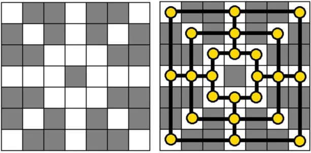
3) The last representation is a three-dimensional object made by 3 matrix of size 3x3 which represents the three concentric squares of the grid. The center of each matrix is a not relevant element. Figure 3.5 presents such representation.

Figure 3.5 3D representation of the board state. The three colors, yellow, orange and red, differentiate the elements belonging respectively to the inner, the middle and the outer

square of the board. The grey elements are not relevant.

Each point of the grid can assume three states: occupied by a white checker, occupied by a black checker or empty. So it’s easy to represent the possible states of a point of the board with 3 different values, for example (1, -1, 0) or (W, B, E).

An important aspect to underline is that, as illustrated in Figure 3.6, none of the suggested representations of the board are capable to capture the concept of logical distance between two board points. For logical distance between two points is meant how much two points are distant according to the game rules and in this case can be defined by the minimum number of moves that are necessary for a checker to move from one point to another during phase 2.

1) Obviously the 1-dimensional representation cannot preserve the logical distance because imposes a linearization of the positions.

2) The 2-dimensional representation fails because weight differently the distance of two points of the same square according to which is the square: the distance between two logically adjacent points of the inner square will be 1, while the distance between two adjacent points in the middle one will be 2 and in the outer one will be 3: there is an overestimation of some distances.

(26)

3) The 3-dimensional representation fails because the points in the same angles of two different squares are represented at the same distance as the points in the midpoint of the same side of two different squares, but while the midpoint are linked so their distance is 1 or 2, the angles are not linked so their distance is 3 or 4: there is an underestimation of some distances.

Figure 3.6 Differences between logical distance (in blue) and “physical” distance (in red) in the 2D representation (left) and the 3D representation (right) of the board

Representation of a move

With the term “move” is meant the whole set of choices that a player takes during his turn.

A very peculiar characteristic that make this problem different from many other board games is that a move is defined by a variable amount of information.

For the entire game, an information that is always needed to define a move is where a player want to place his checker, this can be represented with the coordinates of that point. The coordinates of a point of the grid can be a single number, a couple or a triplet, according on the chosen board representation. This information will be referred to as the “TO” move part and will always be present in the move.

In case that placing the checker causes the closing of a mill, another information that must be represented is the checker that the player wants to remove. This can be represented using the coordinates of the point where the checker is. This information will be referred to as the “REMOVE” move part and is the least frequent part in the move: during a single match, the

(27)

maximum number of moves with a REMOVE part is 13, 7 by the winning player and 6 by the losing one.

Finally, during phase 2 and 3, the checker is moved from a position to another, so another information is where the checker is moved from, one more time this information is a point of the grid so can be represented with the coordinates. This information will be referred to as the “FROM” move part.

So a move is defined by 1 to 3 coordinates among which only the first one is always present. For this reason a special point must be defined, a point that will be addressed by the EAT and FROM part in case the move do not require them.

It is important to underline that for any game state there are constraints on each part itself, but there are also constraints on the whole move: the legality of the parts does not guarantee the legality of the full move.

3.3 Comparison with other board games

It is useful to analyse briefly other popular strategy board games, with the aim of finding similarities and differences with Nine Men’s Morris, in order to make considerations about which of the techniques that will be used in this case of study could be used for other games.

All the games examined are perfect-information games played by two players.

Draughts

Draughts or Checkers is another very wide-spread game, but unlike Nine Men’s Morris, which rules are almost the same everywhere, rules of Draughts change very much depending on the place where is played: Polish draughts, Canadian checkers, Russian draughts, English draughts and Italian draughts are only a few examples of the many different traditional versions [14].

For this reason is difficult to compare precisely those two games: between different versions change the size of the board, the number of checkers and, more important, what are the possible legal moves.

What can be said for all versions is that the board is a squared checkerboard, so it can be easily represented as a 2-dimensional object, preserving the logical distance between two points and without the introduction of

(28)

non-relevant objects. There is not the possibility to have checkers on hand, so the board representation is sufficient to represent the game state; an example of game state is presented in Figure 3.7.

Figure 3.7 Example of game state in international draughts

Another difference is that the definition of legal moves is the same for the whole game, but there are two types of checkers, Men and Kings, which can do different moves; so a point on the board can assume 5 possible states. The last important difference is that a move is defined by at least two points: the checkers that a player wants to move and the position where that checker will be moved. In the case of a move that captures more than one adversary checker, the move is defined also by the points in which the checker passes. So a move is formed by a variable number of parts, but if in Nine Men’s Morris the parts that form a move are semantically a syntactically different, each part of a Draughts move has the same meaning as the others.

The game can end when a player loses either because he cannot make legal moves or because all his checkers are captured; each version of Draughts has its own conditions to determine the end in a draw, but substantially the game is declared a draw if none of the player has the possibility to win or if a certain state is reached many times. So while it is possible to determine if a player has won simply looking at the state, for detecting a draw it could be necessary to maintain history of the states.

The state-space complexity changes between different versions: for example for the English draughts is estimated an upper bound of 1020 [15], while for the international International draughts the upper bound is 1030 [16]. The English version has been weakly solved [17], which means that not only the

(29)

game-theoretic values of the starting position is known, but a strategy to achieve it is known as well.

In 1994, the computer program Chinook won the Checkers World Championship, achieving the title of first program to win a human world championship [18]. Chinook knowledge consisted of a library of opening moves, an incomplete end-game database and a move evaluation function which were used by a deep search algorithm to choose the best move. All this knowledge was programmed by Chinook creator, rather than obtained through machine learning.

Chess

Chess is different from Nine Men’s Morris under almost any aspect.

The chess board is an 8x8 checkerboard so, as has been said for draughts, can be easily represented as a 2-dimensional object, with all the positive aspects previously mentioned, and example of representation is shown in Figure 3.8. One more aspect in common with draughts is the presence of 6 different types of pieces and each one can do a different types of moves.

Figure 3.8 Example of game state in chess

A move is always defined by only two points, the one in which the piece is and the one in which the piece move, with a notable exception: the player who moves a pawn to the end of the board must decide the piece in which he wants the pawn get promoted to, but this decision occurs very few times during a game.

(30)

For almost any aspects, the chess board embodies the game state and the definition of legal moves remain the same for the whole game, the exception to this statement is the castling move. The castling move it’s a special move that the king can do with an allied tower, only under certain conditions of the board and only if none of the two has been moved since the beginning of the game, so it’s important to maintain these information in the game state. The castling move can still be represented with two points: for example the position of the king and of the chosen tower.

The game ends with a winner when a player is under checkmate, which means that his king is threatened with capture and there is no way to remove that threat, so that player have lost. The game ends with a draw if a player has no legal move possible (stalemate) or if none of the player can put the other in checkmate, this is possible if only some pieces remains on the board. These conditions are detectable simply looking at the state.

It is possible to end a game with a draw, under a player request, if one of two conditions occur: for 50 consecutive moves no pawn have been moved and no pieces has been captured or if the same state is reached for the third time (even not consecutively). The second condition is moreover relevant in an AI vs AI game, because it is possible for the players to remain stuck in a loop, so it is important to maintain a history of the game state.

The state-space complexity for chess has not been calculated precisely yet, the upper bound estimated by different authors vary between 1043 and 1050 [16]; due to its high complexity, chess is still an unsolved game.

IBM’s computer Deep Blue was able to won a game against human world champion Kasparov in 1996 and to won a 6 game match the following year. Deep Blue relied on a vast resource of knowledge, such as a database of opening games played by past grandmasters, and applied a brute force approach, exploring that knowledge to figure out the best move. During the state search, the program considered the pieces on the board, their position, the safety of the King and the progress toward vantage states; the evaluation of all these components was made following the behaviour defined by the programmers, without the possibility to change it or adapt it to the opponent strategy [19].

“Kasparov isn't playing a computer, he's playing the ghosts of grandmasters past.” [19]

(31)

Othello

Othello is the easiest game to model between the ones which has been analysed so far.

In Othello the board is a squared plane of size 8x8, so once again it can be represented as a 2-dimensional object, but like in Nine Men’s Morris, only one type of checker exists.

Figure 3.9 Initial game state in Othello

The board is sufficient to represent the game state, as illustrated in Figure 3.9, the definition of legal moves remain the same for the whole game and a move can be represented simply by a point on the board.

An important characteristic is that if a player cannot make a legal move, he must pass the turn, while in the games analysed so long the impossibility for a player to make a legal move meant the end of the game.

When none of the players can make a legal move, the game ends, and the player who has more checkers wins. So the end of the game can be detected simply by analysing the game state.

The state-space complexity has been estimated to be 1028 [16] and it is still mathematically unsolved.

The first Othello program computer able to won a single match against a human world champion was “The Moor” in 1980 [16], while in 1997 the program “Logistello” won a six games match against the human world champion.

(32)

Logistello relied upon a table-based pattern evaluation: to each occurrence of each pattern in each game state corresponded a value that would be added to the state value if those conditions were met. The search through the state space considered not only the best move but also some possible deviations, allowing the system to learn from his games [20].

Go

The game of Go is a very ancient oriental strategy board game. As for

Draught, the wide diffusion of this game among centuries has led to the born of many different versions of the rules. Only the basic rules are considered here.

The game board is a grid made by 19x19 lines, even if it is possible to play with smaller boards, therefore it is easy to represent it with a 2-dimensional object, as shown in Figure 3.10.

Figure 3.10 Example game state in go

During his turn, a player may pass or place a “stone” on the board, so a move can be represented simply by the position where the stone will be placed, using an illegal coordinate to indicate the choice to pass.

(33)

For the whole game the definition of legal move is the same, but it is illegal to recreate a board state which has occurred previously, so in order to define legal moves, it is important to maintain an history of the game states.

The game ends when both player passed and the outcome is determined by the last board configuration.

For this reason, the state of the game could be defined by the board state, the set of previously reached board configuration and the last move made by a player.

Go is probably the most complex traditional board game, because its complexity has been estimated to be 10172 [16] and is still unsolved.

The computer program FUEGO [21] is considered one of the best open source go computer player [22], it uses symbolic techniques like Alpha-Beta Search and Monte Carlo Tree Search to explore the possibile moves and to choose the better one.

(34)

Chapter 4

4 Artificial Neural Networks

Artificial Neural Networks (so forth called neural networks or simply networks) have a long history, which goes back to the first studies on computational models of biological neural networks by McCulloch and Pitts in 1943 [23]. Through time, many models have been proposed, different either in the architecture of the network or in the elements that constitute it or in the training techniques.

Partially inspired by the biological neuron model, as illustrated in Figure 4.1, Neural Networks are a sub-symbolic approach to the problem of learning. Made by many simple units linked together, neural networks store the learned knowledge into the connections between these units as a numerical weight and into other parameters.

Figure 4.1 Simplified models of biological neuron and artificial neuron. The biological neuron gather impulses/inputs through dendrites, aggregates them in the soma and

(35)

In a neural network, a neuron is a computational unit that receives a set of inputs 𝑥_𝑖, elaborates a weighted sum with weights 𝑤_𝑖 and adds a bias 𝑏, than applies an activation function 𝑓 to compute the output 𝑦. Each neuron has therefore as many parameters as the number of inputs plus one.

The output of each neuron can therefore be written as 𝑌(𝑋) = 𝑓 (∑ 𝑥_𝑖𝑤_𝑖

𝑖

+ 𝑏)

where 𝑥_𝑖 are the neuron inputs, while 𝑤_𝑖 and 𝑏 are the parameters to be learned.

A typical activation function is the sigmoid function, but other possible activation functions will be discussed later. The plotting of this function is presented in Figure 4.2, while its definition is:

𝑆(𝑡) = 1 1 + 𝑒−𝑡

Figure 4.2 Sigmoid function plotting

4.1 Feed-forward model and network supervised

training

In the feed-forward neural network model, neurons are grouped in layers, stacked one on top of the other. Therefore, the first layer of neurons (input units), receive the data as input, while the others (hidden units) receive the output of the previous layer as input. The output of the network is made by the outputs of each neuron that belongs to the last layer (output units). A scheme of a possible artificial neural network is presented in Figure 4.3.

(36)

Figure 4.3 Feed-forward neural network architecture scheme

For any given data, the network calculate an output based on his parameters and hyper-parameters. Training a network means to alter these parameters with the aim to make the outputs of the network similar to the desired outputs or, more formally, to optimize a loss function 𝐿 that has to measure the discrepancy between the output of the network and the target.

Gradient descent and backpropagation

If the activation function is differentiable, the gradient descent can be applied to optimize the loss function: the gradient of the loss function with respect to each parameter is computed, than the parameters are modified by the gradient multiplied by an hyper-parameter 𝛼, called learning rate. An iteration on the whole training set, and the related gradient computation, is called training epoch.

By applying this technique many times over the same data, it is possible to reach a local minimum of the loss function. The choice of the learning rate can dramatically influence the training: a small learning slows down the training and could make impossible to escape from a local minimum once it is reached, on the other hand an high learning rate could alter the weights too much on each gradient computation, making the global minimum impossible to reach.

If the activation function is not linear and is differentiable, it is possible to train the network using the backpropagation technique [24]. The idea behind

(37)

backpropagation is to do a two-steps process: a propagation phase and an updating phase.

During the forward propagation the data are given as input to the network and the output 𝑜_𝑗 of each neuron is kept in memory; during the backward propagation the error on the output is calculated and propagated backwards, computing the error 𝛿_𝑗 associated to each neuron.

It is possible to compute the gradient of the loss function of any parameter of network following the chain rule: calling 𝑝𝑎𝑟_𝑗 a parameter of the j-th neuron and 𝑛𝑒𝑡_𝑗 the input to its activation function so that 𝑜_𝑗 = 𝑓(𝑛𝑒𝑡_𝑗), it results

𝜕𝐿 𝜕𝑝𝑎𝑟_𝑗 = 𝜕𝐿 𝜕𝑜_𝑗 𝜕𝑜_𝑗 𝜕𝑛𝑒𝑡_𝑗 𝜕𝑛𝑒𝑡_𝑗 𝜕𝑝𝑎𝑟_𝑗 = 𝛿𝑗 𝜕𝑛𝑒𝑡_𝑗 𝜕𝑝𝑎𝑟_𝑗 Where 𝛿_𝑗 is the error associated to the neuron and 𝜕𝑛𝑒𝑡𝑗

𝜕𝑝𝑎𝑟𝑗 can be defined for the weights and the bias of the neuron as

𝜕𝑛𝑒𝑡_𝑗 𝜕𝑤_𝑖𝑗 = 𝜕(∑ 𝑜_𝑘 _𝑘𝑤_𝑘𝑗 + 𝑏_𝑗) 𝜕𝑤_𝑖𝑗 = 𝑜𝑖 𝜕𝑛𝑒𝑡_𝑗 𝜕𝑏_𝑗 = 𝜕(∑ 𝑜_𝑘 _𝑘𝑤_𝑘𝑗 + 𝑏_𝑗) 𝜕𝑏_𝑗 = 1

During the updating step it is thus possible to compute the gradient of the loss function with respect to each network parameter and finally apply the gradient descent.

Training process

Testing the trained network on the same data used for training could provide a misleading result: the networks performance could be good even in presence of overfitting. To verify the ability of the network to generalize, it is a common practice to split the dataset into two subsets: the training set and the test set.

During training it could be necessary to adjust some hyper-parameters, so it could be useful to test the network after each epoch of training. It is also important to underline that almost every network training will lead to an high overfitting, so it is important to stop the training at the right moment, a technique which is called early stopping.

The training set therefore could be divided into two subsets: the actual training set that will be used for training and a validation set, that will be used

(38)

for testing after each epoch. This division can be defined for the whole training or can change within an epoch; for example the k-fold cross-validation technique divides the training set into k partitions of the same size, during an epoch it does k training steps using one partition for validation and the others for training, computing the error and the accuracy scores as an average over the scores obtained in each step.

Monitoring the performance of the network over the validation set is possible to determine if the network is improving or has already reached its maximum performance and therefore the training can be stopped.

The amount of data used to calculate the gradient, and therefore to update the parameters, have repercussion on the accuracy and the speed of the training. Computing the gradient over the whole training set (batch optimization) could require a great amount of time, therefore it is common to use mini-batch optimization, that means to compute the gradient only on a small subset of the data. The smaller the subset, the more inaccurate is the gradient estimation, but the faster is the gradient computation, so it will probably require more estimation but they will be faster. If the size of the batch is one, the gradient is computed independently for each training example; the approach is called stochastic optimization.

Softmax classifier and negative log likelihood loss

In classification tasks or, more generally, if the output of the network must be one class out of many, it is a very common practice to put a softmax classifier as last layer of the network [25]. The softmax function takes a set of real values as input, which are considered as un-normalized log probabilities, and map them into normalized probabilities.

More formally, calling 𝑓_𝑗(𝑥) the score computed by the network for the class 𝑗 with the provided input 𝑥, the probability 𝑃 that the input 𝑥 should be labelled as 𝑘 is:

𝑃(𝑌 = 𝑘, 𝑥) = 𝑒

𝑓_𝑘(𝑥)

∑ 𝑒𝑓𝑗(𝑥) 𝑗

From this probability score is possible to obtain a loss score computing the negative log likelihood.

(39)

In information theory the difference between a true distribution 𝑡(𝑥) and a distribution 𝑝(𝑥) can be evaluated with the cross-entropy between them, which is defined as:

𝐻(𝑡, 𝑝) = − ∑ 𝑡(𝑥) log 𝑝(𝑥)

𝑥

If as 𝑡(𝑥) is considered a distribution where all probability mass is on the correct class, so it is formed by only zeros except a 1 on the correct class, and as 𝑝(𝑥) is considered the probability distribution resulting from the softmax function, the result is the negative log likelihood of the correct class 𝑘, which will be used as loss function:

𝐿_𝑘 = − log 𝑃(𝑌 = 𝑘, 𝑥) = − log ( 𝑒 𝑓𝑘(𝑥) ∑ 𝑒𝑓𝑗(𝑥) 𝑗 )

Regularizations

Two common regularization penalties used in the loss function are the L1 and L2 norms, which discourage the use of large weights in the network to obtain a more general model. The penalty is added to the loss function with a weight λ which is an hyper-parameter of the training. Calling 𝑊_𝑖,𝑗 the weight of the connection between neurons 𝑖 and 𝑗, the two penalties are defined as:

𝑅_𝐿2(𝑊) = ∑ ∑ 𝑊_𝑖,𝑗2 𝑗 𝑖 𝑅_𝐿1(𝑊) = ∑ ∑|𝑊_𝑖,𝑗| 𝑗 𝑖

Learning rate annealing

On one hand a low learning rate requires many epochs of training to reduce the error significantly, but on the other hand a high learning rate slows down or prevents the system from achieving highest accuracy.

The solution to this problem is the learning rate annealing, which means to reduce the learning rate after some epochs of training, obtaining an heavy and fast error reduction at first and a slow but constant one later.

(40)

Many learning rate annealing techniques have been designed:

 Step decay: every few epochs the learning rate is reduced by some factor, for example it can be halved every 10 epochs, or divided by 10 every 20 epochs.

 Exponential decay: an initial learning rate 𝛼₀ is established, than the learning rate for each epoch is defined as 𝛼 = 𝛼₀𝑒−𝑘𝑡, where 𝑡 is the epoch and 𝑘 is an hyper-parameter

 Proportional decay: similar to the previous one, but the learning rate is defined as 𝛼 = 𝛼0

(1+𝑘𝑡)

Ensemble learning

To achieve better results, it is a common machine learning technique to train more than one model and use them together to achieve better results. In bagging ensemble [26] all the models are trained independently and contribute equally to the final prediction, while in boosting ensemble [27] each model is trained with the aim of fixing the errors of the previous ones. In the case of neural networks, it is possible to train different models on the same data changing the architecture or an hyper-parameter, or train the same model on different data, or even use the same model trained on the same data but for a different amount of epochs.

4.2 Historical background

To better understand which are the problems which concerns modern networks and how they have been addressed, it useful to present the evolution of neural networks technologies since their invention.

Neuron and perceptron model

In 1943, McCulloch and Pitts presented the first mathematical model based on human neurons [23]. The artificial neuron took a weighted sum of inputs with weight equals to +1 or -1 and applied a threshold; the output was binary, with value 1 if the sum is greater than 0, with value 0 otherwise.

That model was than improved by Frank Rosenblatt, who proposed the Perceptron Algorithm in 1957 [28]:

𝑓(𝑥) = {1 𝑖𝑓 𝑤 ∗ 𝑥 + 𝑏 > 0 0 𝑜𝑡ℎ𝑒𝑟𝑤𝑖𝑠𝑒

(41)

The activation function was a binary step function, so it was not-differentiable and therefore backpropagation was impossible; the update rule did not take into account any loss function or similar, indeed it was simply defined as:

𝑤_𝑖(𝑡 + 1) = 𝑤_𝑖(𝑡) + 𝛼(𝑑_𝑗 − 𝑦_𝑗(𝑡))𝑥_𝑗𝑖

The perceptron was physically implemented into a machine designed for image recognition called Mark 1 Perceptron. Few years later, in 1960, Widrow and Hoff stacked together many single units creating the first multilayer perceptrons: Adeline and Madaline.

In 1969, Minsky and Papert wrote a book [29] in which they analysed the limits of the perceptron: they are able to solve only linearly separable problems, for example they underlined the impossibility to learn the XOR function, even though multilayer perceptron have not these limitations.

Backpropagation, CNNs and DBNs

Even if some progress was made during the sequent years, that book caused a general lack of interest in the research on perceptron, which last until 1986, when backpropagation was defined clearly [24] and became popular, greatly improving neural networks performances.

The problem concerning neural networks still was that they were not scalable: an high number of layers or an high number of neurons in a layer brought to worse performance.

LeNet-5, a Convolutional Neural Network for handwritten and machine-printed character recognition, was realized in 1989 [30] and improved during the following decades.

Designed specifically for computer vision tasks, convolutional neural networks have a different architecture: each neuron represented the convolution between the image of the previous layer and a filter, therefore the neurons of a layer were distributed along three dimensions and were connected to only few of neurons of the previous and of the successive layer. The learnable parameters of the network were the weights used in the convolution, which were shared between many neurons of the same layer. In this way the network resulted more independent from the size of the input image and therefore scaled better.

(42)

In 2006 Deep Belief Networks were presented, combining supervised and unsupervised training to achieve better results in a 2 step process [31]: firstly couples of adjacent layers were trained to reconstruct the input through Restricted Boltzman Machines, than the whole network was fine-tuned with backpropagation.

The key of the success of this process resided in the first step: the unsupervised training initialized the parameters of the network, partially preventing the sigmoid function from saturating.

4.3 Deep Networks and recent approaches

In the last years, enthusiasm for neural networks has risen once again, probably due to a great results obtained in 2010 in speech recognition [32] and another one obtained in 2012 in image classification, when the network AlexNet [33] won the ImageNet Large Scale Visual Recognition Challenge classification task [34].

The success of neural networks still continue, indeed since 2012 the ILSVRC classification task has always been won by neural networks, which have also been successfully used in many other computer vision task [34].

These impressive achievements have been made possible thanks to new models and techniques which have been studied in the last 5 years.

Rectified Linear Unit

The use of the sigmoid function has many downsides: it has two saturation zone in which the gradient is annealed, his mean is not zero and the computation of the exponential operator could be very expensive.

Further studies on biological neurons and the advantages of sparsity have led to the definition of an alternative model of the artificial neuron [35], which has been successfully tested in convolutional networks performing supervised training tasks [36].

The rectifier neuron, also called ReLU (REctified Linear Unit), uses the rectifier activation function, which is plotted in Figure 4.4 and defined as: