2020-12-22T10:52:29Z
Acceptance in OA@INAF
Active galactic nuclei vs. host galaxy properties in the COSMOS field
Title
LANZUISI, Giorgio; DELVECCHIO, IVAN; Berta, S.; Brusa, M.; COMASTRI,
Andrea; et al.
Authors
10.1051/0004-6361/201629955
DOI
http://hdl.handle.net/20.500.12386/29092
Handle
ASTRONOMY & ASTROPHYSICS
Journal
602
Number
A&A 602, A123 (2017) DOI:10.1051/0004-6361/201629955 c ESO 2017
Astronomy
&
Astrophysics
Active galactic nuclei vs. host galaxy properties
in the COSMOS field
?
G. Lanzuisi
1, 2, I. Delvecchio
3, S. Berta
4,??, M. Brusa
1, 2, A. Comastri
2, R. Gilli
2, C. Gruppioni
2, S. Marchesi
2, 5,
M. Perna
1, 2, F. Pozzi
1, 2, M. Salvato
6, M. Symeonidis
7, C. Vignali
1, 2, F. Vito
8, M. Volonteri
9, and G. Zamorani
2.
1 Dipartimento di Fisica e Astronomia, Università di Bologna, Viale Berti Pichat 6/2, 40127 Bologna, Italy
e-mail: [email protected]
2 INAF–Osservatorio Astronomico di Bologna, via Ranzani 1, 40127 Bologna, Italy 3 Department of Physics, University of Zagreb, Bijeniˇcka cesta 32, 10002 Zagreb, Croatia
4 Department of Physics, Faculty of Science, University of Zagreb, Bijeniˇcka cesta 32, 10000 Zagreb, Croatia 5 Department of Physics & Astronomy, Clemson University, Clemson, SC 29634, USA
6 Max-Planck-Institut für extraterrestrische Physik, Giessenbachstrasse, 85748 Garching, Germany
7 Mullard Space Science Laboratory, University College London, Holmbury St. Mary, Dorking, Surrey RH5 6NT, UK
8 Department of Astronomy and Astrophysics, 525 Davey Laboratory, The Pennsylvania State University, U. Park, PA 16802, USA 9 Institut d’Astrophysique de Paris, UPMC et CNRS, UMR 7095, 98bis Bd Arago, 75014 Paris, France
Received 25 October 2016/ Accepted 22 February 2017
ABSTRACT
Context.The coeval active galactic nuclei (AGN) and galaxy evolution, and the observed local relations between super massive black holes (SMBHs) and galaxy properties suggest some sort of connection or feedback between SMBH growth (i.e., AGN activity) and galaxy build-up (i.e., star formation history).
Aims.We looked for correlations between average properties of X-ray detected AGN and their far-IR (FIR) detected, star forming host galaxies in order to find quantitative evidence for this connection, which has been highly debated in recent years.
Methods.We exploited the rich multiwavelength data set (from X-ray to FIR) available in the COSMOS field for a large sample (692 sources) of AGN and their hosts in the redshift range 0.1 < z < 4. We use X-ray data to select AGN and determine their properties, such as X-ray intrinsic luminosity and nuclear obscuration, and broadband (from UV to FIR) SED fitting results to derive host galaxy properties, such as stellar mass (M∗) and star formation rate (SFR).
Results.We find that the AGN 2–10 keV luminosity (LX) and the host 8−1000 µm star formation luminosity (LSFIR) are significantly
correlated, even after removing the dependency of both quantities with redshift. However, the average host LSF
IRhas a flat distribution
in bins of AGN LX, while the average AGN LXincreases in bins of host LSFIRwith logarithmic slope of ∼0.7 in the redshift range 0.4 <
z< 1.2. We also discuss the comparison between the full distribution of these two quantities and the predictions from hydrodynamical simulations. No other significant correlations between AGN LXand host properties is found. On the other hand, we find that the
average column density (NH) shows a clear positive correlation with the host M∗at all redshifts, but not with the SFR (or LSFIR). This
translates into a negative correlation with specific SFR at all redshifts. The same is true if the obscured fraction is computed.
Conclusions.Our results are in agreement with the idea, introduced in recent galaxy evolutionary models, that SMBH accretion and SFRs are correlated, but occur with different variability time scales. Finally, the presence of a positive correlation between NHand
host M∗suggests that the column density that we observe in the X-rays is not entirely due to the circumnuclear obscuring torus, but
may also include a significant contribution from the host galaxy.
Key words. galaxies: active – galaxies: nuclei – galaxies: evolution – infrared: galaxies – X-rays: galaxies
1. Introduction
Super massive black hole (SMBH) growth and galaxy build up follow a similar evolution through cosmic history, with a peak at z ∼2−3 and a sharp decline toward the present age (see Madau & Dickinson2014, for a review). Furthermore, at z= 0, SMBH and their hosts sit on tight relations that link the SMBH mass and the bulge properties of the host, such as luminosity, stel-lar mass, and velocity dispersion (Kormendy & Richstone1995; Magorrian et al.1998; Kormendy & Ho2013). Therefore SMBH
? Full Table 1 is only available at the CDS via anonymous ftp to
cdsarc.u-strasbg.fr(130.79.128.5) or via
http://cdsarc.u-strasbg.fr/viz-bin/qcat?J/A+A/602/A123
?? Visiting scientist.
growth and star formation history are likely related in some way during the cosmic time.
The key parameter that regulates both processes seems to be cold/molecular gas supply (Lagos et al.2011; Vito et al. 2014; Delvecchio et al.2015; Saintonge et al.2016). Processes related to star formation (e.g., supernova and stellar winds) are known to produce galaxy-wide outflows that can regulate the in-fall of gas and therefore star formation itself (e.g., Genzel et al.2011). However, more powerful mechanisms, globally known as “AGN feedback”, have been invoked in numerical and semi-analytic models of galaxy evolution (e.g., Granato et al.2004; Di Matteo et al.2005; Menci et al.2008; Sijacki et al.2015; Dubois et al. 2016; Pontzen et al.2017) in order to reproduce the observed galaxy population, and particularly the high mass end of the galaxy mass function.
Observationally, the role of AGN activity in influencing the evolution of the global galaxy population is not clear yet. This is-sue has been investigated, and correlations searched for between average AGN and host properties, such as BH accretion rates (BHAR) or AGN luminosity (typically in the 2−10 keV band; hereafter LX) on the one hand, and star formation rates (SFRs)
or IR luminosity (in the 8−1000 µm; hereafter LIR) on the other
hand, taking advantage of the wealth of multiwavelength infor-mation collected in deep extragalactic surveys. However, di ffer-ent, somewhat contradictory results have been reported in recent years.
Several studies have found a flat distribution computing av-erage LIR in bins of LXof X-ray selected sources (or SFR and
BHAR, respectively, e.g., Shao et al.2010; Rovilos et al.2012; Rosario et al. 2012) at low redshift and luminosities. A sig-nificant positive correlation instead appears for luminous AGN (LX> 1043−44erg s−1) and high redshifts (z > 1−2), suggesting
two different triggering mechanisms at high and low luminosi-ties, via merger and secular evolution, respectively.
Other groups have found a linear correlation at all z and LX
when computing the average LXin bins of LIR(in log-log space)
of IR selected sources (Chen et al.2013; Delvecchio et al.2015; Dai et al. 2015), with the ratio Log (SFR/BHAR) ∼ 3, roughly consistent with the local Mbulge/SMBH value (Magorrian et al.
1998; Marconi & Hunt2003). Finally, other authors have found no correlation at all, regardless of the LX and z range (e.g.,
Mullaney et al.2012; Stanley et al.2015).
Looking at AGN obscuration, Rovilos et al. (2012) explored for the first time the possible relation between AGN column den-sity (NH), as measured from the X-ray spectra, and host
proper-ties, and found no correlation on a sample of 65 sources in the XMM-CDFS survey (Comastri et al.2011). Rosario et al. (2012) found similar result from hardness ratios (HR) on a larger sam-ple in COSMOS, while Rodighiero et al. (2015) found a positive correlation between NHand M∗, again based on HR, on a sample
of z ∼ 2 AGN hosts in the same field.
From a technical point of view, these differences may partly arise from different biases and analysis methods. For example, given that only a small fraction of the X-ray detected sources are far-IR (FIR) detected, and vice versa, most of these stud-ies rely on X-ray or FIR stacking in order to recover the av-erage properties of large samples of AGN/host systems, or are limited to small subsamples. Mullaney et al. (2015) pointed out that modeling the SFR distribution of X-ray selected hosts as a log-normal distribution, and including upper limits, gives dif-ferent results than computing the linear mean of the distribution (i.e., via stacking), which is instead driven upwards by the bright outliers.
Another issue was raised by Symeonidis et al. (2016), who showed that the intrinsic AGN SED in the FIR is cooler than usu-ally assumed. Therefore, in some cases there is no “safe” pho-tometric band which can be used to calculate the SFR without subtracting the AGN contribution. On the other hand, several of the works cited above take the FIR photometry directly (typically at 60 µm) in order to estimate SFR, thus potentially introducing a spurious correlation at high AGN luminosities.
Recently, from theoretical studies, a physical mechanism has been proposed to explain part of these contradictory results. Volonteri et al. (2015a,b) explain that these different observa-tions are due to the way we analyze the data: the bivariate dis-tribution of AGN and SF luminosities gives two very di ffer-ent results depending on the binning axis used. Hickox et al. (2014) reached similar conclusions starting from the simple as-sumptions that long-term AGN activity and SFR are perfectly
correlated, that the observed SFR is the average over ∼100 Myr, while the AGN activity, traced by X-ray emission, varies on much shorter time scales. In these models the different time scales involved in AGN and SF variability dilute the linear de-pendency between the two quantities if the rapidly variable AGN luminosity is used to build the subsamples to be studied “on av-erage”. This result was also confirmed observationally by Dai et al. (2015) using shallow data from XMM-LSS.
Furthermore, Volonteri et al. (2015a) suggest that spatial scales are important; the BH accretion rate should be lated with the nuclear (<100 pc) SFR, while it is less corre-lated with the total (<5 kpc) SFR, except for the most intense merger episodes, which are able to affect the whole host galaxy. Of course, the SFR that can be inferred from the FIR luminosity is the global, galaxy-scale SFR (with the exception of the local Universe; see, e.g., Diamond-Stanic & Rieke2012), and this in-troduces another source of uncertainty in the observational com-parison between BHAR and SFR.
Here we explore the possible correlations between AGN and host properties for a large sample of X-ray and FIR detected sources thanks to the extensive Chandra, XMM–Newton, and Herschelcoverage on the COSMOS field (Scoville et al.2007; Hasinger et al.2007; Elvis et al.2009; Lutz et al.2011; Oliver et al. 2012). This approach avoids the uncertainties related to the stacking, and allows for a proper SED deconvolution, source by source. This of course limits the significance of our findings to the brightest, most accreting, and most star forming systems. These systems are, however, the most interesting ones, the ones for which there is less agreement in the literature on the pres-ence of a correlation between AGN and SF, and also the ones for which theoretical models predict that the correlation should be stronger.
The paper is organized as follows: Sect. 2 describes the sam-ple and source properties; Sect. 3 presents the analysis of LX
and LIR distributions; in Sect. 4 we compare our results with a
set of hydrodynamical simulations; in Sect. 5 we discuss cor-relations between nuclear obscuration and host properties and in Sect. 6 we discuss our results. Throughout the paper we as-sume a standardΛCDM cosmology with H0= 70 km s−1Mpc−1,
ΩΛ= 0.73, and ΩM= 0.27 (Bennett et al.2013).
2. Sample
We performed X-ray spectral fitting for all the Chandra and XMM–Newton detected sources (from the catalogs of Brusa et al. 2010; and Civano et al. 2015, respectively) with more than 30 counts, in Marchesi et al. (2016) and Lanzuisi et al. (2013, 2015), respectively. This sample consist of 2333 indi-vidual sources (1949 Chandra and 1187 XMM–Newton sources, with 803 source in common1).
For all the Herschel detected sources in the COSMOS field (∼17 000 with at least a detection at >3σ in one of the FIR bands, from 100 to 500 µm; Lutz et al.2011), an SED deconvolu-tion with three components – stellar emission, AGN torus emis-sion, and SF-heated dust emission – performed using photomet-ric points from the UV to sub-mm, is available from Delvecchio et al. (2014,2015; hereafter D15), following the recipe described in Berta et al. (2013).
We then selected all the XMM–Newton and Chandra de-tected sources that have at least one FIR detection (and therefore SED deconvolution). The final sample comprises 692 X-ray and
1 The Chandra data from Marchesi et al. (2016) are used for the
G. Lanzuisi et al.: AGN vs. host properties in COSMOS
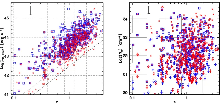
Fig. 1.Left: distribution of rest frame, absorption-corrected 2–10 keV luminosity vs. redshift for the XMM–Newton (blue squares) and Chandra (red crosses) detected sources that are also Herschel detected (X-FIR sample). The dotted (dashed) line marks the sensitivity limit of the XMM– Newton(Chandra) surveys. The redshift bins adopted in the text are marked by vertical gray dashed lines. Right: distribution of intrinsic column density vs. redshift for the sample. Symbols as in left panel. Arrows show upper limits for unobscured sources. The average 1σ error bars on LX
and NHare shown at the top left of both panels.
FIR detected sources (hereafter the X-FIR sample), 459 spec-troscopic and 233 photometric, all of them with an available redshift (Civano et al. 2012; Brusa et al. 2010; Salvato et al. 2009; Marchesi et al. 2015). To date this is the largest sample of AGN/host systems for which X-ray spectral parameters, such as column density and absorption-corrected 2–10 keV luminos-ity, are known in combination with host properties such as M∗
and SFR.
2.1. AGN properties
Figure1, (left) shows the distribution of LXvs. redshift for the
X-FIR sample. The average 1σ error bar on LXis shown in the
upper left corner. The absorption-corrected LXis affected by
un-certainties related to both the number of net counts (observed flux uncertainties) and the spectral shape of each source (un-certainties on NHand spectral slope). Therefore, the errors have
been derived, for each source using the equivalent in Sherpa (Fruscione et al.2006) of the cflux model component in Xspec (Arnaud1996), applied to the best-fit unabsorbed power law. The flux and errors are then computed in the observed band corre-sponding to 2–10 keV rest frame, and converted into luminosity. The redshift bins that will be used in the following analysis are shown with vertical dashed lines. The intervals have been chosen with the aim of having a fairly large number of sources in each bin (∼80−160) with a reasonably narrow redshift interval. The LXbins that will be used in the following (1 bin per dex) are
shown as horizontal dashed lines.
Figure1, (right) shows the column density distribution for the X-FIR sample. Arrows show sources for which the obscura-tion is constrained only by an upper limit. The average 1σ error bar on NH is shown in the upper left corner. The distribution
of NHfrom X–ray spectral analysis has a clear upper boundary
around Compton Thick (hereafter CT) column densities2due to the strong flux decrement associated with CT obscuration in the 2–10 keV band. Also, the minimum measurable NH increases
with redshift as the low energy cutoff due to obscuration move outside the observing band.
The global fraction of X-ray obscured sources (those with NH> 1022 cm−2) in the X-FIR sample is ∼50%, higher than the
typical obscured fraction (30–40%) of the X-ray samples in the Chandra- and XMM–Newton-COSMOS (Lanzuisi et al. 2015; Marchesi et al.2016). Indeed, the FIR luminosity (and therefore Herscheldetection rate) of type-2 AGN seems to be higher than for type-1 QSO (Chen et al.2015).
2.2. Host properties
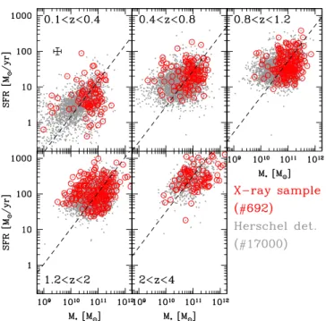
The host properties (SFR vs. M∗) of the 692 sources in the X-FIR
sample are shown in Fig.2 (red circles) divided into five red-shift bins as described above. The values are taken from D15: the SFR has been derived by converting the IR luminosity (rest 8−1000 µm) of the best-fitting galaxy SED (i.e., subtracting the AGN emission when present) with the SF law of Kennicutt (1998), scaled to a Chabrier (2003) initial mass function (IMF). The M∗is derived from the SED decomposition itself, and based
on Bruzual & Charlot (2003) models, with a consistent IMF. Table 1 (full version available at the CDS) summarizes the mul-tiwavelength properties of the sources in the X-FIR sample.
The host properties of the sample of Herschel detected sources (from D15, ∼17 000 sources) are shown for compari-son with gray dots. The average of the statistical 1σ error bars resulting from the SED fit3 are shown in the top left corner.
2 Lanzuisi et al. (2015a,b) present the CT sources detected by XMM–
Newton, while Lanzuisi et al. (in prep.) will present the ones detected by Chandra.
3 Systematic errors like uncertainties related to the adopted IMF or SF
Fig. 2.SFR vs. M∗distribution for the entire sample of Herschel
de-tected sources (∼17 000 sources, gray points) and for the 692 sources with X-ray spectral analysis (X-FIR sample, red circles), divided into the five redshift bins defined in Sect. 2.1. The dashed lines in each panel mark the redshift-dependent MS of Withaker et al. (2012). The average 1σ error bars are shown in the top left as a black cross.
The errors on M∗ follow a log-normal distribution, with
aver-age herr(M∗)i = 0.14 dex and standard deviation σ = 0.09.
The mean error on SFR is herr(SFR)i = 0.10 dex, and stan-dard deviation of σ = 0.07 as for LSFIR (see Sect. 3.1), since the SFR is derived from LSFIR adopting a Kennicutt (1998) law. The redshift-dependent MS of star forming galaxies, as described in Whitaker et al. (2012), is also shown in each panel. The FIR selected sources broadly follow the MS relation. However, the Herschel-based selection is sensitive to the most star forming systems, introducing a cut in SFR that moves towards higher val-ues with increasing redshift (e.g., Rodighiero et al.2011, D15).
X-ray detected AGN are preferentially found at the highest M∗, i.e., the fraction of X-ray detected sources increases as a
function of M∗, in the first three redshift bins at least. This is a
well-known effect (Kauffmann et al.2003; Bundy et al. 2008; Brusa et al.2009; Silverman et al.2009; Mainieri et al. 2011; Santini et al.2012; Delvecchio et al.2014). Aird et al. (2012) suggested that it is the result of an observational bias, such that more massive galaxies (i.e., more massive BHs) can be detected at a given X-ray flux limit with a variety of accretion rates, while lower mass systems can be detected only if they have a high accretion rate. This, combined with a steep Eddington ratio dis-tribution (i.e., sources with low Eddington ratio are much more common than sources with high Eddington ratio) can explain the observed M∗distribution (see also Bongiorno et al.2012).
In our case there is a threshold at around log M∗∼ 10.5 M
in the first 3 redshift bins. A simple calculation shows that this value can be roughly derived from the X-ray flux limit of the Chandra and XMM–Newton surveys using standard val-ues for bolometric corrections (kBol = 10−30), Eddington
ratios (λEdd∼ 0.05), and BH-host mass ratios (M∗/MBH =
1000−3000). A more detailed study of the Eddington ratio dis-tribution that can be derived from the M∗ and LX distributions
will be presented in Suh et al. (2017).
Several studies in the local Universe suggest that the fraction of galaxies hosting an AGN also increases with IR luminosity (e.g., Lutz et al. 1998; Imanishi et al.2010; Alsonso-Herrero et al. 2012; Pozzi et al.2012). We also tested that the observed threshold in mass is not driven by our requirement of Herschel detection; when using the M∗-SFR distribution of Bongiorno
et al. (2012), computed for the full XMM-COSMOS catalog, a drop in the number of X-ray detected AGN below log M∗= 10.2–
10.4 M is visible up to z= 2.5.
The consequence of this selection effect is that the X-FIR sample has a M∗distribution shifted toward higher M∗with
re-spect to the global Herschel sample (Fig.3, top right); instead, the distribution of SFR for the X-FIR sample is roughly consis-tent with that of the global Herschel sample (Fig. 3, top left). This has important implications when measuring sSFR and MS offsets, for example (Fig. 3, bottom left and right): due to this selection effect the X-FIR sample has lower sSFR with respect to the MS of star forming galaxies (or to the Herschel sample) if the two samples are not properly mass-matched (Silverman et al. 2009; Xue et al.2010).
3. LXvs. LIR distributions 3.1. Partial correlation analysis
The two quantities that have been used most often to look for BHAR-SFR correlations are the AGN luminosity, often repre-sented by LX, and the SF luminosity in the form of LIR(or L60 µm;
Santini et al.2012; Rosario et al.2012; Chen et al.2013). It is generally assumed that the total FIR luminosity is not signifi-cantly affected by any contamination from the AGN emission. However, recent studies have shown that AGN may contribute significantly to the IR emission and in some cases even in the FIR band (Symeonidis et al.2016). Therefore, the SFR derived directly from FIR photometry can be overestimated, especially in high luminosity AGN hosts. Thanks to the SED decomposi-tion available, we use in the following the LIR computed only
for the SF component (hereafter LSFIR), after subtracting the AGN contribution, modeled with the SED templates of Fritz et al. (2006; see also Feltre et al.2012). This avoids introducing a spu-rious correlation between AGN and SF luminosity, especially at the highest luminosities.
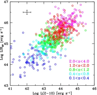
Clearly two luminosities are always correlated in any sample that is flux limited in both directions, due to the combination of the luminosity-distance effect and tendency of the sources to cluster at the flux limit (Malmquist bias, e.g., Feigelson & Berg1983). Figure4shows the distribution of LXvs. LIRfor the
X-FIR sample.
The 1σ errors on LSF
IR follow a log-normal distribution with
average value herr(LSF
IR)i = 0.10 dex, and standard deviation
of σ = 0.07. As mentioned in Sect. 2.1, the errors on the absorption-corrected luminosity follow a much broader distri-bution depending on the number of counts available and on the spectral shape. They range from <∼0.1−0.2 dex for bright, unobscured sources, to ∼0.5−1.0 dex for faint and highly ob-scured sources. The average value of the 1σ error is herr(LX)i ∼
0.23 dex, with standard deviation σ= 0.18. We show the aver-age errors with a black cross in the left panel of Fig.4, while the specific value for each source is used in the following analysis.
In order to look for intrinsic correlations between these two quantities, one possibility is to compute the partial Spearman rank correlation between two variables in the presence of a third, and to assess the statistical significance of such correlation (e.g., Macklin1982). To derive the correlation coefficient between LX
G. Lanzuisi et al.: AGN vs. host properties in COSMOS
Fig. 3.Fractional distribution of the host properties, SFR, M∗, sSFR, and MS offset, from top left to bottom right, for the X-FIR sample (black
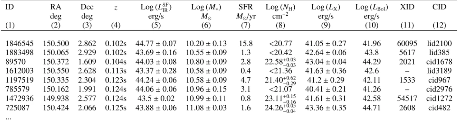
open histogram) and for the whole Herschel sample (gray filled histogram), in redshift bins. Table 1. Multiwavelength properties of the 692 sources in the X-FIR sample.
ID RA Dec z Log (LSF
IR) Log (M∗) SFR Log (NH) Log (LX) Log (LBol) XID CID
deg deg erg/s M M /yr cm−2 erg/s erg/s
(1) (2) (3) (4) (5) (6) (7) (8) (9) (10) (11) (12) 1846545 150.500 2.862 0.102s 44.77 ± 0.07 10.20 ± 0.13 15.8 <20.77 41.05 ± 0.27 41.96 60095 lid2100 1883498 150.065 2.929 0.102s 43.69 ± 0.16 10.55 ± 0.09 1.3 <20.42 42.64 ± 0.06 43.8 5617 lid385 89570 150.372 1.609 0.104s 44.03 ± 0.08 10.80 ± 0.09 2.8 22.58+0.03−0.03 43.04 ± 0.04 44.29 2021 cid1678 1612003 150.550 2.628 0.113s 43.37 ± 0.28 10.58 ± 0.09 0.4 <21.36 41.63 ± 0.36 42.6 – lid3189 1197519 150.335 2.304 0.123s 44.24 ± 0.06 10.58 ± 0.09 4.7 21.40+0.62−0.29 41.2 ± 0.29 42.11 1533 cid967 785579 150.162 1.991 0.124s 44.06 ± 0.06 10.96 ± 0.15 3.1 <21.07 40.41 ± 0.21 41.26 – cid2976 1472936 149.938 2.577 0.124s 43.5 ± 0.02 10.99 ± 0.11 0.8 23.11+0.15−0.16 41.61 ± 0.31 42.58 54517 cid1272 725087 150.424 2.066 0.125s 43.88 ± 0.06 11.08 ± 0.03 1.6 24.26+0.05−0.04 43.36 ± 0.35 44.71 2608 cid482 ...
Notes. Catalog entries are as follows: (1) Source ID from Capak et al. (2007); (2) and (3) right ascension and declination of the optical/IR
counterpart; (4) redshift (s for spectroscopic or p photometric); (5) Log (LSF
IR) with 1σ errors; (6) Log (M∗) with 1σ errors; (7) SFR derived from
LSF
IR; (8) Log (NH) with 1σ errors or upper limits; (9) Log (LX) with 1σ errors; (10) Log (LBol) computed from LX using Marconi et al. (2004);
(11) and (12) XMM-COSMOS and Chandra-COSMOS IDs (from Brusa et al.2010; and Marchesi et al.2016, respectively). The full table is available at the CDS.
and LSFIR, conditioned by the distance, ρ(LX, LSFIR, ˙z), we evaluate
the Spearman coefficient ρ related to each pair of parameters and then combine them according to the expression
ρ(a, b, ˙c) = ρab−ρcaρbc
q (1 − ρ2
ca)(1 − ρ2bc)
(1)
(Conover 1980), which returns the partial correlation between a and b, corrected for the dependency on c. The resulting ρ is 0.15, and the associated confidence level, in terms of standard devia-tions, that the first two variables are correlated, independently of the influence of the third, is ∼3.7σ, following Eq. (6) of Macklin (1982). Therefore, the two quantities appear to be significantly
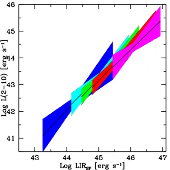
Fig. 4.LXvs. LSFIRfor the X-FIR sample. Different colors represent
dif-ferent redshift bins: blue for 0.1 < z < 0.4, cyan for 0.4 < z < 0.8, green for 0.8 < z < 1.2, red for 1.2 < z < 2, and magenta for 2 < z < 4. The average 1σ errors on LXand LSFIRare shown in the upper left corner.
correlated, after the effect of redshift on both of them is taken into account.
3.2. Redshift bins
The second approach, often used in the literature, is to define redshift bins that are as narrow as possible to minimize the dis-tance effect, and to look for correlations between the two quan-tities. Thanks to the large sample collected in this work, we can divide the sample into five redshift bins. For every redshift bin, a large distribution in both luminosities can be observed, with the typical luminosity increasing with redshift (Fig.4).
Most of the observational works mentioned in Sect.1looked for the distribution of average LSFIR in LX bins, or average LX
in LSFIR bins (but see Gruppioni et al.2016). Both hydrodynami-cal simulations (e.g., Volonteri et al.2015a,b) and semi-analytic models (e.g., Neistein & Netzer2014) show that, in the LSF
IR-LX
plane, there may be the superimposition of a weak correlation for the bulk of the population, and a strong correlation only for the most extreme merger phases, corresponding to the highest LXand LSFIR. If the underlying distribution shows such a complex
shape, the results of the two approaches (average LSF
IR in LXbins
or average LXin LSFIR bins) may be very different.
In Fig.5(left) we show the result of plotting average LSFIR in bin of LX(both in log scale) in five redshift bins. As can be seen,
there is no correlation at all LSF
IR and, as expected, there are no
sources below the relation computed for a pure AGN template in Mullaney et al. (2011), similar to the one used in Netzer et al. (2009). Following this approach, we are therefore able to repro-duce the results of Shao et al. (2010), Rosario et al. (2012), and others that claim no correlation between AGN activity and SF over several orders of magnitude in luminosity.
On the other hand, computing average LX in LSFIR bins (in
log scale) from the same bivariate distribution gives different results. Figure 5 (right) shows that at all redshifts the average LX correlates with the LSFIR and the binned points are close to
the SFR/BHAR ∼ 500 ratio found in Chen et al. (2013; hereafter C13).
In both panels, we computed the error on the average LXand
LSF
IR through a bootstrap re-sampling procedure, as done in
sev-eral previous works. For each bin with N sources, we randomly extract N sources, allowing repetitions, and computed the mean value. The process is iterated 104times, and the standard
devia-tion of the mean is taken as the error on the average SFR. The two approaches described above are the equivalent of computing the forward and inverse linear regression of one vari-able over the other. Tvari-able 2 reports the slopes α and intercept β, and their associated errors, for each redshift bin in the log-log space of the least-squares (LS) fit4 of LSF
IR as a function of
LX(hereafter LSFIR | LX), and LXas a function of LSFIR (hereafter
LX| LSFIR ), respectively5. Indeed, the slopes in the left panel are
all consistent with 0 within ∼2σ confidence level. On the other hand, LS fits of (LX| LSFIR ) give steeper correlations at all z bins
and slopes not consistent with 0 at ∼ 3σ confidence level. The SFR/BHAR ∼ 500 ratio plotted in Fig.5 is the value found in C13 for a sample of 121 FIR selected AGN-hosts at 0.25 < z < 0.8. For a comparison with their results we should look at our first two z-bins: While the z-bin 0.1 ≤ z < 0.4 has a very flat (LX|LSFIR ) slope, possibly due to the small volume
sam-pled, the 0.4 ≤ z < 0.8 interval shows a correlation with slope consistent with 1 at ∼ 1σ, therefore in broad agreement with the C13 findings. Interestingly, we can extend up to 0.8 ≤ z < 1.2 the redshift range for which a correlation roughly consistent with SFR/BHAR ∼ 500 can be found. Above this redshift interval, the slopes become flatter. Therefore, we found a strong (almost lin-ear) correlation between log LX and log LSFIR for (LX | LSFIR ) at
redshifts lower than the peak of the SF and AGN activity, i.e., between 4 and 8 Gyr ago, while at higher redshift the correlation is still present but weaker.
The exact value of the ratio SFR/BHAR in terms of LXand
LSF
IR depends strongly on the assumptions made to scale between
these quantities, i.e., the accretion efficiency and bolometric cor-rection in the first case, and the SF law and initial mass func-tion (IMF) in the second. Chen et al. (2013) derived the SFR from LSFIR using the Kennicutt (1998) relation modified for a Chabrier IMF (Chabrier2003), and the BHAR from LXusing
a constant kbol = 22.4 and accretion efficiency of 0.1. They
use as reference the value of SFR/BHAR ∼ 500 derived from the
MBulge/MBHratio observed in Marconi et al. (2004). The authors
suggest it is a coincidence that the detected sources sit on the SFR/BHAR ∼ 500 ratio, due to the ratio between the X-ray and FIR flux limits in the Boötes field.
In the X-FIR sample in COSMOS we have a factor of ∼10 deeper X-ray data (taking into account the flux limit cor-responding to our spectral analysis requirements), while the Herscheldata are only a factor of 2–3 deeper (∼8 mJy at 110 µm and 8 mJy at 250 µm) than in Boötes. Nonetheless, our X-FIR detected sample sit close to the C13 relation. We note that in both cases the X-ray and FIR detected sources are a small minor-ity of both the original X-ray and FIR samples (a small percent, up to ∼20%), and the flux limit has an important role in the ob-served properties of the detected sources alone, as also discussed in C13.
4 The LS fit is performed with the BCES code (Akritas & Bershady
1996), adopting 104bootstrap re-samplings. Similar results are obtained
using the LINMIX code (Kelly et al.2007).
5 In the first case slopes and intercepts refer to a relation in the form
Log LSF
IR= 45 + α × (Log LX−44)+ β, while in the second in the form
G. Lanzuisi et al.: AGN vs. host properties in COSMOS
Fig. 5.Left: average Log (LSF
IR) in bins of Log (LX) in five redshift bins. The short dashed line is the correlation derived in Mullaney et al. (2011)
for a pure AGN SED. Right: average Log (LX) in bins of Log (LSFIR). The long dashed line represents a constant SFR/BHAR of 500, from C13. In
both panels the vertical error bars are computed through a bootstrap resampling procedure, while the horizontal error bars show the 1σ dispersion of that bin.
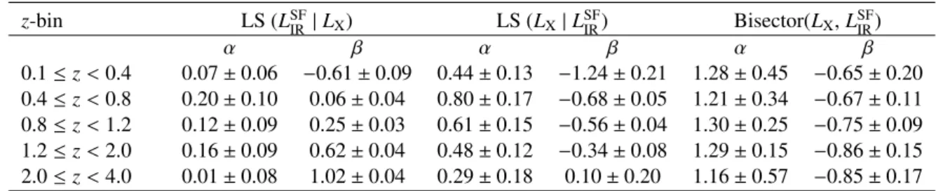
Table 2. Slopes α and intercept β of the linear LS fit of (LSF
IR| LX), (LX| LSFIR), and of the bisector estimator in each redshift bin.
z-bin LS (LSF IR | LX) LS (LX| LSFIR) Bisector(LX, LSFIR) α β α β α β 0.1 ≤ z < 0.4 0.07 ± 0.06 −0.61 ± 0.09 0.44 ± 0.13 −1.24 ± 0.21 1.28 ± 0.45 −0.65 ± 0.20 0.4 ≤ z < 0.8 0.20 ± 0.10 0.06 ± 0.04 0.80 ± 0.17 −0.68 ± 0.05 1.21 ± 0.34 −0.67 ± 0.11 0.8 ≤ z < 1.2 0.12 ± 0.09 0.25 ± 0.03 0.61 ± 0.15 −0.56 ± 0.04 1.30 ± 0.25 −0.75 ± 0.09 1.2 ≤ z < 2.0 0.16 ± 0.09 0.62 ± 0.04 0.48 ± 0.12 −0.34 ± 0.08 1.29 ± 0.15 −0.86 ± 0.15 2.0 ≤ z < 4.0 0.01 ± 0.08 1.02 ± 0.04 0.29 ± 0.18 0.10 ± 0.20 1.16 ± 0.57 −0.85 ± 0.17
Notes. The first set of slopes and intercepts refers to a relation in the form Log LSF
IR= 45 + α × (Log LX−44)+ β, while the second and third in the
form Log LX= 44 + α × (Log LSFIR−45)+ β.
As discussed in Hickox et al. (2014) and Volonteri et al. (2015), a possible physical explanation for this behavior is that we are averaging a slowly changing quantity, such as the host SFR, of galaxies grouped on the basis of the rapidly changing AGN LX(see Fig.5, left panel). In the right panel, instead, the
average LX of a large sample of sources grouped on the basis
of the slowly changing SFR allows us to recover the underly-ing, long-term correlation between AGN activity and SFR. In the same way, from a statistical point of view, it may be reasonable to interpret the LXas the dependent variable in this context as it
has larger uncertainties with respect to LSF
IR (Hogg et al.2010),
both in terms of measurement errors (see Sect. 3.1) and noise (i.e., variability).
If we instead assume that in this case there are no “depen-dent” and “indepen“depen-dent” variables (see, e.g., Tremaine et al. 2002; Novak et al. 2006), the two variables may need to be treated symmetrically. We used the BCES code again to derive slope and intercept, and their standard deviation, using a sym-metric estimator such as the bisector regression6 (Isobe et al. 1990). The results are shown in Fig. 6, while the slopes and
6 We recall that the BCES estimators, both the LS and the symmetric,
are not immune from biases that arise from data truncation, which is the case for flux-limited samples (see Akritas & Bershady1996).
intercepts are listed in Table 2. At all redshift bins, the slopes of the linear regression, although always larger than 1, are con-sistent with 1 within a 1σ confidence level.
3.3. Effect of contamination
Since the Herschel PACS and SPIRE point spread functions (Pilbratt et al. 2010) are much larger than those in the optical and NIR bands, going from ∼500 to ∼3600 FWHM (Poglitsch
et al.2010; Griffin et al.2010), there is the possibility that the FIR flux of our sources is contaminated by unresolved neighbors (see, e.g., Scudder et al.2016).
We verified the effect of contamination by excluding all the X-FIR sources with a second HST catalog entry from the ACS F814W(I-band) catalog (28.6 AB limiting magnitude, Scoville et al.2007; Koekemoer et al.2007). We choose a circular area of diameter 800around the optical position. While this distance is
not great enough to ensure negligible contamination, it has been chosen in order to retain a sufficient number of sources to allow an analysis in all five redshift bins. The 146 “isolated” sources obtained in this way show the same behavior described above, with a flat distribution of average LSF
Fig. 6.Linear regression for LXand LSFIRcomputed for each redshift bin
with the bisector estimator in BCES. The color code is the same as in Fig.4.
and an almost linear correlation of average LXcomputed in bin
of LSFIR.
We also verified that sources with a single PACS or SPIRE detection (more subject to contamination) do not affect our re-sults. Indeed, excluding the 154 (out of 692) sources with only one detection (at 3σ) either in PACS or SPIRE photometry does not change the results presented in Sect. 3.2 and in the following paragraphs.
3.4. LBol, M∗, sSFR, and MS offset
Several authors have used the AGN bolometric luminosity (LBol), instead of the LX, to look for correlation with the LIR
or SFR. The LBolis generally derived from the LXthrough a
lu-minosity dependent bolometric correction (e.g., Marconi et al. 2004; Lusso et al.2012). The net effect of this procedure is to stretch the horizontal axis of Fig.5 (left) (the high LXsources
have a higher X-ray bolometric correction than the low LXones),
while keeping the LSFIR fixed. In Fig.7we show the result of this approach (here we used the Marconi et al.2004, luminosity de-pendent bolometric correction, but the Lusso et al.2012, relation would have the same effect): in each redshift bin the sources pop-ulating the highest LXbin are now spread in two LBolbins, and
the last LBol bin at each redshift is now populated by a smaller
number of more extreme sources. The relation found locally for AGN-dominated systems in Netzer et al. (2009) is also shown. Once again, we are able to reproduce results obtained in other works (Shao et al.2010; Rosario et al.2012). However, we are now confident that this result is not in disagreement with what is shown in Fig.5(right) and the apparent contradiction is only de-pendent on the way the data are analyzed and grouped, as shown in e.g., Volonteri et al. (2015) and discussed in Stanley et al. (2015) and Dai et al. (2015).
Finally, we found a flat distribution when computing average LXin bins of M∗, sSFR, and MS offset and average M∗, sSFR,
and MS offset in bins of LXin all five redshift bins. Indeed, no
significant partial correlation is found between any pair of these quantities following the approach described in Sect. 3.1 to take
Fig. 7.Average Log (LSF
IR) in bin of LBol, for the X-FIR sample. The
dashed line is the relation found in Netzer et al. (2009) for AGN-dominated systems. Error bars are computed as in Fig.5.
into account the redshift effect, which also affects M∗, SFR, and
sSFR (σ 1 in all cases). We stress, however, that the range of M∗ covered by our sample is limited to the very high mass
end, 10 < Log (M∗) < 12 (to be compared with the underlying
galaxy M∗ distribution, 7 < Log (M∗) < 12, in the same redshift
interval shown in e.g., Laigle et al. 2016). Deeper X-ray surveys are needed to investigate the dependency of LXwith this crucial
quantity.
4. Theory and observations 4.1. Comparison with simulations
Here we compare our results with predictions from the simu-lations of galaxy mergers presented in Volonteri et al. (2015a). They are based on very high spatial and temporal resolution sim-ulations, covering a wide range of initial mass ratios (1:1 to 1:10), several orbital configurations, and gas fraction (defined as Mgas/M∗) in the range fgas = 0.3−0.6. The very high
resolu-tion imposes a limit on the mass of the simulated galaxies, which typically have M∗∼ (2−8) × 109 M , i.e., much smaller than the
typical mass of our observed galaxies (see Fig.3). The process is divided into three phases: the stochastic phase, which lasts until the second pericenter, where the galaxies behave as they do in isolation; the merger phase characterized by strong dy-namical torques and angular momentum loss; and the remnant phase, which starts when the angular momentum returns to be constant in time. While the stochastic and remnant phases have the same duration (by construction), the merger phase is much shorter (typically 1/10 of the total).
To compare our data with this set of simulated galaxies, we converted the AGN bolometric luminosity into a BH mass ac-cretion rate (BHAR), by assuming an efficiency of η = 0.1 (e.g., Fabian & Iwasawa1999) and dividing it by the host stellar mass to obtain a specific BHAR (sBHAR) relative to the host mass rather than to the BH mass. We chose to do so because, from an observational point of view, the determination of the M∗ (from
G. Lanzuisi et al.: AGN vs. host properties in COSMOS
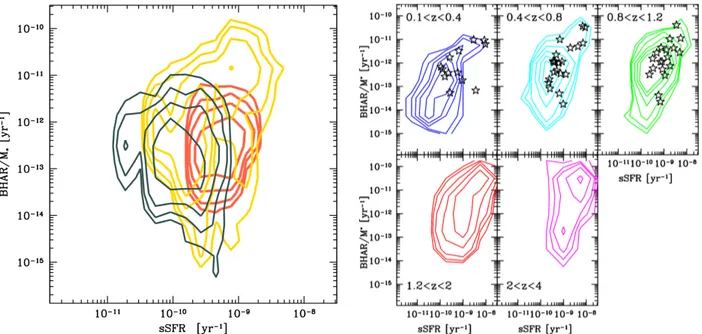
Fig. 8.Left: BHAR/M∗rate vs. sSFR contours obtained from the simulations presented in Volonteri et al. (2015a). In red the stochastic phase, in
yellow the merger phase, and in black the remnant phase. Right: BHAR/M∗vs. sSFR contours observed in COSMOS in five redshift bins. Sources
that are in a major merger state in the first three redshift bins are marked with black stars.
budget in our sample) than that of MBH, and is available for both
type-1 and type-2 AGN. This value is then compared with the sSFR for each source. The contours of global (within 5 kpc) sSFR vs. sBHAR obtained from the simulations for the three dif-ferent phases (stochastic, merger, and remnant), are color-coded in Fig.8(left) in red, yellow, and black, respectively.
The results from the X-FIR sample are shown in Fig.8(right) for the five redshift bins. As can be seen the observed contours in the low redshift bins span a similar range of physical proper-ties, with respect to simulations, with the bulk of the population concentrated between 5 × 10⁻¹¹and 5 × 10⁻⁹yr−1in sSFR, and between 10−14and 10−11yr−1in sBHAR, and with a tail at higher
sSFR and sBHAR, possibly produced by sources in the merger phase as in the simulations (yellow contours). Interestingly, the importance of this tail grows with increasing redshift, even if the selection effect in both directions must be taken into account.
We also exploited the deep HST ACS coverage in the COS-MOS field to identify sources in the merger phase. We only se-lected sources that appear to be in a clear major merger phase, and overplotted them in Fig. 8(right) as black stars in the first three redshift bins (above z ∼ 1 it becomes difficult to assess the AGN host morphology). This selection is not meant to be complete: not all the sources are covered by ACS, and it is not possible to recognize the host morphology for all of them, due to bright point-like AGN contribution, for example. However, it is interesting that AGN hosts clearly in merger state tend to cover the highest sSFR and sBHAR range, as predicted by simulations.
4.2. Caveat
One caveat to be considered here is the fact that the simula-tions are performed at high-z, starting at z= 3 and ending after 1−3 Gyr depending on the merger dynamics (see Capelo et al. 2015, for details). By construction, the simulations have a rel-atively low gas fraction: 30% of the disk stellar mass. This is probably a low value for SF galaxies at these redshifts. Only one set of simulations has been performed with a higher gas fraction (60%) and, as expected, these simulated galaxies move toward
higher sSFR and sBHAR, as the contours of the observed high redshift sample do.
Another caveat is the fact that the simulations are performed for low mass galaxies. The typical M∗ for these galaxies is in
the range Log (M∗)= 9–9.5 (M ), i.e., in the low mass tail of the
mass distribution even for the lowest redshift bin of the observed sample. Since the efficiency of SFR and BHAR is most prob-ably mass-dependent, the comparison between different mass ranges may not be straightforward. Volonteri et al. (2015a) ar-gue, however, that SFR and BHAR are self-similar, on the basis of the mass sequence of star forming galaxies and of the possible power-law dependence of the specific BHAR (Aird et al.2012; Bongiorno et al. 2013, but see Kauffmann & Heckman 2009; Lusso et al.2012; and Schulze et al.2015).
Finally, the simulations are not cosmological, in the sense that the gas mass is not replenished by cosmic inflows and gas accretion, as is the case for real galaxies. This leads to a possible underestimate of SFR and BHAR towards the end of the simu-lation when galaxies have converted a large fraction of their gas into stellar and BH mass (see also Vito et al.2014).
5. Obscuration
5.1. NHand host properties
Here we discuss the possible correlations between the column density through the AGN line of sight, as measured by the X-ray NH, and the host galaxy properties, such as M∗, SFR, sSFR, and
MS offset. The partial correlation analysis described in Sect. 3.1 gives a significant positive correlation (at >4σ confidence level) between NHand M∗in the entire sample once the distance effect
is removed (both NH and M∗ tend to increase with redshift in
two different ways, due to two different selection effects). We also find a significant negative correlation (at >5σ confidence level) between NHand sSFR, while we do not find any significant
correlation of NHwith SFR and MS offset.
As in the case of LXvs. LIR, the binning direction (or the
vari-able chosen as independent) is relevant for the final distribution of NHas a function of host properties and vice versa: computing
Fig. 9.Linear regression of NHvs. M∗(left) and sSFR (right) in five redshift bins. The regression is performed using the linmix code, which also
takes into account the NHupper limits. The color-coding is the same as in Fig.4. The gray squares in the left panel show results from Rodighiero
et al. (2015) at z ∼ 2, obtained from the HR of X-ray stacked images of FIR detected galaxies in the COSMOS field. The orange dashed line is the relation found in Buchner et al. (2017) for a sample of GRB hosts in a wide range of redshifts (see text).
average SFR, M∗, sSFR, and MS offset in bins of NHwe found a
remarkably flat distribution of all these quantities, in agreement with results from Shao et al. (2010), Rovilos et al. (2012), and Rosario et al. (2012), where the authors do not find any evolution of the average host properties in bins of NH.
On the other hand, computing average NHvalues in bins of
M∗ gives a positive trend in each redshift bin, while computing
the average NH in sSFR bins gives a negative trend, in
agree-ment with partial correlation analysis. However, the situation in this case is complicated by the presence of upper limits in NH,
that makes the problem inherently asymmetric. We therefore per-formed the linear regression of (Y|X) with a Bayesian approach using the linmix code (Kelly et al.2007), which is able to prop-erly take into account the upper limits on NH.
The result is shown in Fig.9: the linear regression gives a clear positive correlation of NH with the host stellar mass,
in-creasing by 1–2 dex from low to high masses at all redshifts (slopes in the range α= 0.42–0.88). An opposite result is found for the sSFR: the average NHdecreases typically by one order of
magnitude or more, going from low to high sSFR (slopes in the range α= −0.35–−0.82). Given that there is no trend of NHwith
SFR, and that the sSFR is defined as SFR/M∗, the two relations
are clearly connected.
A similar result between NHand M∗was found in Rodighiero
et al. (2015) for a sample of z ∼ 2 AGN hosts. In their analysis, however, the average NHis globally ∼1 dex higher (gray squares
in Fig.9, left) because they derive NHfrom the hardness ratio of
the X-ray stacking, which also includes highly obscured, unde-tected AGN.
Interestingly, a recent study on the distribution of the ob-scuration observed in X-ray spectra of GRB, as a function of the host galaxy mass, found a similar trend in the redshift range 1 <∼ z <∼ 5 (Buchner et al.2017, orange line in Fig.9, left). Since for these sources the NHfrom the GRB spectra probes only the
host obscuration, the authors conclude that a large fraction of the obscuration observed in AGN, at least in the Compton thin
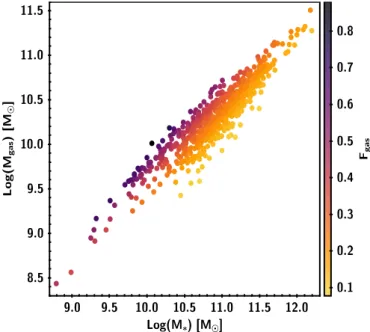
Fig. 10.log M∗vs. log Mgasas derived from Eq. (1) of Scoville et al.
(2016). The sources are color-coded on the basis of their gas fraction.
regime, is not due to the nuclear torus, but to the galaxy-scale gas in the host.
These dependencies imply that at increasing galaxy mass there are more chances to have an additional component to the amount of gas and dust along the line of sight through the AGN. It is well established that the gas fraction is a strong decreasing function of the galaxy mass (e.g., Santini et al.2014; Peng et al. 2015). However, it is possible to show that the total amount of gas is driven mainly by the total galaxy mass and not by the gas fraction. To this end, we computed gas mass for all our galaxies, following the empirical relation found in Scoville et al. (2016) (their Eq. (1)), that links M∗, sSFR offset from the MS, and
G. Lanzuisi et al.: AGN vs. host properties in COSMOS
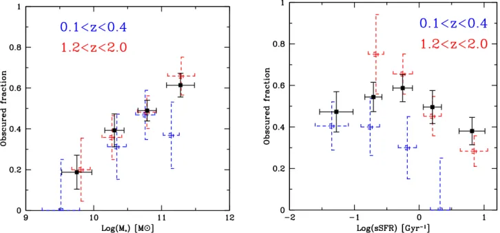
Fig. 11.Fraction of obscured sources as a function of M∗(left) and sSFR (right), for the entire sample (black points). The blue (red) dashed points
show the results for the first (fourth) redshift bin, respectively.
are color-coded on the basis of their gas fraction. Even if at in-creasing M∗the gas fraction is smaller, the total amount of gas
still increases with M∗.
The well-known mass-metallicity relation (e.g., Tremonti et al.2004; Mannucci et al.2010) goes in the direction of having more metals (responsible for X-ray absorption) with increasing M∗. In particular, going from Log (M∗)= 9.5 to 11.5, there is an
increase of a factor ∼2 in the metallicity, up to z ∼ 2 (Erb et al. 2006); however, this is not enough to explain the increase in av-erage NHobserved here. Measuring the NHwith fixed
metallic-ity (as is done here) for sources with such a range in metallicmetallic-ity translates into a factor of ∼2 difference in measured NH for a
given input obscuration.
5.2. Obscured fraction
To compare our results with the literature, we also looked at the fraction of obscured sources as a function of host proper-ties. In Fig. 11 we show the fraction of obscured sources, de-fined as NObs/NTot, where NObs is the number of sources with
a detection of NH and NH> 1 × 1022 cm−2. As expected from
what was shown in the previous section, the fraction of obscured sources increases with increasing M∗ and decreases with sSFR
(for sSFR > 1 Gyr−1). The decrease in sSFR is partly hidden
be-cause we consider the full redshift interval (z = 0.1−4), while Fig.9(right) shows that the range covered by the different sub-samples shifts toward higher sSFR with redshift. For this reason we also show in Fig.11the results for the first and fourth bins as an example (blue and red dashed points, respectively).
Merloni et al. (2014) found a flat relation between the frac-tion of obscured sources and M∗ in a sample of X-ray detected
AGN from the XMM-COSMOS catalog. However, they limited their analysis to a narrow range in LX(in order to cover a wide
range redshift), while the obscured fraction is known to evolve strongly with LX(e.g., Ueda et al. 2015).
Another group, instead, have found an increasing fraction of obscured sources as a function of sSFR and MS offset, in a sam-ple of 70 µm selected galaxies at 0.3 < z < 1, interpreted as an indication of increasing gas fraction or density in the host,
which in turn would sustain the increased sSFR (e.g., Juneau et al.2013; hereafter J13).
We note that the definition of obscured AGN adopted here and in J13 are different, and in the latter, are mostly based on the lack of X-ray detection; there are 64 sources (out of 99 AGN) classified as obscured AGN on the basis of the mass-excitation diagram selection (MEX; Juneau et al.2011), and the X-ray non-detection. If these objects are indeed highly obscured, Compton-thick AGN, this population is mostly missed in our X-ray based sample.
Another possibility is that a fraction of the MEX-selected AGN are not actively/strongly accreting SMBHs. Indeed, a siz-able fraction (∼30%) of the AGN selected in J13 through the MEX diagram has a host M∗below Log (M∗)= 10.5. As shown
in Sect. 2.2, however, X-ray detected AGN are rare at low M∗.
Therefore, all the sources that are X-ray undetected for reasons different from obscuration (variability, intrinsic weakness, con-taminant non-AGN, etc.) would appear as obscured, low M∗host
AGN (hence high sSFR), possibly affecting the observed trends.
6. Discussion
We collected a large sample of X-ray and FIR detected AGN and host systems in the COSMOS field, spanning ∼4 orders of magnitude in LX, NH, LSFIR, M∗, and covering the redshift range
0.1 < z < 4. We applied X-ray spectral analysis down to very low counts (>30 net counts) and adopted the SED decomposition results derived in D15, to recover both AGN and SF properties of each source. With this data set in hand, we demonstrated that it is possible to reproduce both the flat distribution of average LSF IR
in bins of LXand the steeper correlation of average LXin bins
of LSF
IR reported in the literature in recent years (e.g., Shao et al.
2010; Rosario et al.2012; Mullaney et al. 2012, C13; Stanley et al.2015).
The apparently contradictory results found in the literature, and reproduced in Sect. 3.2, are due to the different results that are obtained when binning along one axis or the other, the equivalent of a forward or inverse linear regression (i.e., LSF
Volonteri et al. (2015), and found in Dai et al. (2015) and Stanley et al. (2015) (but see also McAlpine et al.2017, for a possible alternative explanation).
Both from a physical and a statistical point of view, it seems more appropriate to consider the results from LX| LSFIR, given the
larger measurement uncertainties on LX, and the shorter time
scale variability of LXwith respect to LSFIR, which adds a further
term of intrinsic scatter. Doing so, we found a linear correlation between LXand LSFIR with a slope consistent with 1, at least in the
redshift range 0.4–1.2, i.e., below the peak of the SF and BH ac-cretion history. Beyond that and up to z= 4, the slope becomes significantly flatter, α= 0.3−0.5.
The other possibility is to adopt a symmetrical approach, even if there is no general agreement on this (see Hogg et al. 2010, on the bisector method). In this case the result is a corre-lation with slope consistent with ∼1 at all redshifts. This would point toward an average one-to-one correlation between SF and BH accretion, in the last 12 Gyr of cosmic history.
Even more interesting is the full distribution of BH and host properties, such as LXand LSFIR or sBHAR and sSFR, that can be
only qualitatively compared, for the moment, with predictions from galaxy merger simulations, resulting in interesting similar-ities between observations and models.
We stress again that these results apply to the small subsam-ple of AGN/host systems detected in both X-ray and FIR, which represents only ∼20% of the full X-ray sample and ∼10% of the AGN FIR sample. Indeed, one of the main reasons why it is so difficult for present observations to probe the AGN-SF connec-tion is that X-ray and/or FIR detected systems span a limited range in AGN and SF activity, sampling only the high LX/SFR
tail of the possible correlation (e.g., Sijacki et al.2015). It is interesting, however, that we are able to reproduce the results obtained via stacking of samples where the vast majority of the sources are not detected (e.g., 20% of FIR detected AGN selected in X-ray in Shao et al.2010). As suggested in Mullaney et al. (2015), the stacking analysis is the equivalent of a linear mean, and may be dominated by the brightest sources.
A crucial next step in the comparison between theory and observations will be to select the observed systems in different evolutionary stage, to reach a similar level of detail as in the cur-rent simulations. This will be feasible for large samples only at low redshift, while detailed and complete morphological stud-ies in COSMOS (and other deep fields) data are already very difficult at z >∼ 1. From the theoretical point of view, more de-manding galaxy merger simulations will be required in order to cover a mass range comparable to the one of observed systems with the same high resolution, and to possibly move toward a high redshift environment.
Finally, a positive correlation between NHand M∗, and a
sim-ilar negative correlation with sSFR, have been found at all red-shift bins. A similar result was found by Rodighiero et al. (2015) in a large sample of high redshift galaxies, computing HR of stacked X-ray images. A recent study on GRB hosts has found a similar behavior (Buchner et al.2017), implying that an impor-tant fraction (up to 40%) of the Compton thin obscuration found in AGN can be ascribed to galaxy scale gas (Buchner & Bauer 2017).
Several studies have found no correlation between column density and host properties (Rovilos et al. 2012; Rosario et al. 2012), while others (e.g., J13) have found a positive correlation of the fraction of obscured sources with sSFR. Further investi-gation in this direction will help to shed light on the role of the host in contributing to the obscuration through the AGN line of sight.
Acknowledgements. The authors thank the anonymous referee for valuable com-ments. G.L., M.B., and M.P. acknowledge financial support from the CIG grant “eEASY” No. 321913. G.L. acknowledges financial support from ASI-INAF 2014-045-R.0. I.D. acknowledges the European Union’s Seventh Framework programme under grant agreement 337595 (ERC Starting Grant, “CoSMas”). We acknowledge the contributions of the entire COSMOS collaboration con-sisting of more than 100 scientists. More information on the COSMOS survey is available athttp://cosmos.astro.caltech.edu/. Based on observations obtained with XMM-Newton, an ESA science mission with instruments and con-tributions directly funded by ESA Member States and NASA, and data obtained from the Chandra Data Archive.
References
Aird, J., Coil, A. L., Moustakas, J., et al. 2012,ApJ, 746, 90 Akritas, M. G., & Bershady, M. A. 1996,ApJ, 470, 706
Alonso-Herrero, A., Pereira-Santaella, M., Rieke, G. H., & Rigopoulou, D. 2012, ApJ, 744, 2
Arnaud, K. A. 1996,Astronomical Data Analysis Software and Systems V, ASP Conf. Ser., 101, 17
Bennett, C. L., Larson, D., Weiland, J. L., et al. 2013,ApJS, 208, 20 Berta, S., Lutz, D., Santini, P., et al. 2013,A&A, 551, A100
Bongiorno, A., Merloni, A., Brusa, M., et al. 2012,MNRAS, 427, 3103 Brusa, M., Fiore, F., Santini, P., et al. 2009,A&A, 507, 1277
Brusa, M., Civano, F. Comastri, A., et al. 2010,ApJ, 716, 348 Bruzual, G., & Charlot, S. 2003,MNRAS, 344, 1000 Buchner, J., & Bauer, F. E. 2017,MNRAS, 465, 4348
Buchner, J., Schulze, S., & Bauer, F. E. 2017,MNRAS, 464, 4545 Bundy, K., Georgakakis, A., Nandra, K., et al. 2008,ApJ, 681, 931 Cai, Z.-Y., Lapi, A., Xia, J.-Q., et al. 2013,ApJ, 768, 21
Capak, P., Aussel, H., Ajiki, M., et al. 2007,ApJS, 172, 99
Capelo, P. R., Volonteri, M., Dotti, M., et al. 2015,MNRAS, 447, 2123 Chabrier, G. 2003,ApJ, 586, L133
Chen, C.-T. J., Hickox, R. C., Alberts, S., et al. 2013,ApJ, 773, 3(C13) Chen, C.-T. J., Hickox, R. C., Alberts, S., et al. 2015,ApJ, 802, 50 Civano, F., Elvis, M., Brusa, M., et al. 2012,ApJS, 201, 30 Civano, F., Marchesi, S., Elvis, M., et al. 2017, ApJ, submitted Comastri, A., Ranalli, P., Iwasawa, K., et al. 2011,A&A, 526, L9 Cresci, G., Hicks, E. K. S., Genzel, R., et al. 2009,ApJ, 697, 115 Dai, Y. S., Wilkes, B. J., Bergeron, J., et al. 2015, ArXiv e-prints
[arXiv:1511.06761]
Delvecchio, I., Gruppioni, C., Pozzi, F., et al. 2014,MNRAS, 439, 2736 Delvecchio, I., Lutz, D., Berta, S., et al. 2015,MNRAS, 449, 373 Diamond-Stanic, A. M., & Rieke, G. H. 2012,ApJ, 746, 168 Di Matteo, T., Springel, V., & Hernquist, L. 2005,Nature, 433, 604 Dubois, Y., Peirani, S., Pichon, C., et al. 2016,MNRAS, 463, 3948 Elvis, M., Civano, F., Vignali, C., et al. 2009,ApJS, 184, 158 Erb, D. K., Shapley, A. E., Pettini, M., et al. 2006,ApJ, 644, 813 Fabian, A. C., & Iwasawa, K. 1999,MNRAS, 303, L34 Feigelson, E. D., & Berg, C. J. 1983,ApJ, 269, 400
Feltre, A., Hatziminaoglou, E., Fritz, J., & Franceschini, A. 2012,MNRAS, 426, 120
Fritz, J., Franceschini, A., & Hatziminaoglou, E. 2006,MNRAS, 366, 767 Fruscione, A., McDowell, J. C., Allen, G. E., et al. 2006,Proc. SPIE, 6270, 1 Genzel, R., Newman, S., Jones, T., et al. 2011,ApJ, 733, 101
Granato, G. L., De Zotti, G., Silva, L., Bressan, A., & Danese, L. 2004,ApJ, 600, 580
Griffin, M. J., Abergel, A., Abreu, A., et al. 2010,A&A, 518, L3 Gruppioni, C., Berta, S., Spinoglio, L., et al. 2016,MNRAS, 458, 4297 Hasinger, G., Cappelluti, N., Brunner, H., et al. 2007,ApJS, 172, 29 Hickox, R. C., Mullaney, J. R., Alexander, D. M., et al. 2014,ApJ, 782, 9 Hogg, D. W., Bovy, J., & Lang, D. 2010, ArXiv e-prints [arXiv:1008.4686],
unpublished
Imanishi, M., Maiolino, R., & Nakagawa, T. 2010,ApJ, 709, 801
Isobe, T., Feigelson, E. D., Akritas, M. G., & Babu, G. J. 1990,ApJ, 364, 104 Juneau, S., Dickinson, M., Alexander, D. M., & Salim, S. 2011,ApJ, 736, 104 Juneau, S., Dickinson, M., Bournaud, F., et al. 2013,ApJ, 764, 176(J13) Kauffmann, G., & Heckman, T. M. 2009,MNRAS, 397, 135
Kauffmann, G., Heckman, T. M., Tremonti, C., et al. 2003,MNRAS, 346, 1055 Kelly, B. C. 2007,ApJ, 665, 1489
Kennicutt, R. C., Jr. 1998,ApJ, 498, 541
Koekemoer, A. M., Aussel, H., Calzetti, D., et al. 2007,ApJS, 172, 196 Kormendy, J., & Ho, L. C. 2013,ARA&A, 51, 511
Kormendy, J., & Richstone, D. 1995,ARA&A, 33, 581
Lagos, C. D. P., Baugh, C. M., Lacey, C. G., et al. 2011,MNRAS, 418, 1649 Lanzuisi, G., Civano, F., Elvis, M., et al. 2013,MNRAS, 431, 978
G. Lanzuisi et al.: AGN vs. host properties in COSMOS Lanzuisi, G., Ranalli, P., Georgantopoulos, I., et al. 2015a,A&A, 573, A137
(L15)
Lanzuisi, G., Perna, M., Delvecchio, I., et al. 2015b,A&A, 578, A120 Lusso, E., Comastri, A., Simmons, B. D., et al. 2012,MNRAS, 425, 623(L12) Lutz, D., Spoon, H. W. W., Rigopoulou, D., Moorwood, A. F. M., & Genzel, R.
1998,ApJ, 505, L103
Lutz, D., Poglitsch, A., Altieri, B., et al. 2011,A&A, 532, A90 Macklin, J. T. 1982,MNRAS, 199, 1119
Madau, P., & Dickinson, M. 2014,ARA&A, 52, 415
Magorrian, J., Tremaine, S., Richstone, D., et al. 1998,AJ, 115, 2285 Mainieri, V., Bongiorno, A., Merloni, A., et al. 2011,A&A, 535, A80 Maiolino, R., Shemmer, O., Imanishi, M., et al. 2007,A&A, 468, 979 Mannucci, F., Cresci, G., Maiolino, R., Marconi, A., & Gnerucci, A. 2010,
MNRAS, 408, 2115
Marchesi, S., Civano, F., Elvis, M., et al. 2016a,ApJ, 817, 34 Marchesi, S., Lanzuisi, G., Civano, F., et al. 2016b,ApJ, 830, 100 Marconi, A., & Hunt, L. K. 2003,ApJ, 589, L21
Marconi, A., Risaliti, G., Gilli, R., et al. 2004,MNRAS, 351, 169
McAlpine, S., Bower, R. G., Harrison, C. M., et al. 2017, MNRAS, 468, 3395
Menci, N., Fiore, F., Puccetti, S., & Cavaliere, A. 2008,ApJ, 686, 219 Merloni, A., Bongiorno, A., Brusa, M., et al. 2014,MNRAS, 437, 3550 Mullaney, J. R., Alexander, D. M., Goulding, A. D., & Hickox, R. C. 2011,
MNRAS, 414, 1082
Mullaney, J. R., Pannella, M., Daddi, E., et al. 2012,MNRAS, 419, 95 Mullaney, J. R., Alexander, D. M., Aird, J., et al. 2015,MNRAS, 453, L83 Neistein, E., & Netzer, H. 2014,MNRAS, 437, 3373
Novak, G. S., Faber, S. M., & Dekel, A. 2006,ApJ, 637, 96 Oliver, S. J., Bock, J., Altieri, B., et al. 2012,MNRAS, 424, 1614 Peng, Y., Maiolino, R., & Cochrane, R. 2015,Nature, 521, 192 Pilbratt, G. L., Riedinger, J. R., Passvogel, T., et al. 2010,A&A, 518, L1
Poglitsch, A., Waelkens, C., Geis, N., et al. 2010,A&A, 518, L2 Pontzen, A., Tremmel, M., Roth, N., et al. 2017,MNRAS, 465, 547 Pozzi, F., Vignali, C., Gruppioni, C., et al. 2012,MNRAS, 423, 1909 Rodighiero, G., Daddi, E., Baronchelli, I., et al. 2011,ApJ, 739, L40 Rodighiero, G., Brusa, M., Daddi, E., et al. 2015,ApJ, 800, L10 Rosario, D. J., Santini, P., Lutz, D., et al. 2012,A&A, 545, A45 Rovilos, E., Comastri, A., Gilli, R., et al. 2012,A&A, 546, A58 Saintonge, A., Catinella, B., Cortese, L., et al. 2016,MNRAS, 462, 1749 Salvato, M., Hasinger, G., Ilbert, O., et al. 2009,ApJ, 690, 1250 Santini, P., Rosario, D. J., Shao, L., et al. 2012,A&A, 540, A109 Santini, P., Maiolino, R., Magnelli, B., et al. 2014,A&A, 562, A30 Schulze, A., Bongiorno, A., Gavignaud, I., et al. 2015,MNRAS, 447, 2085 Scoville, N., Aussel, H., Brusa, M., et al. 2007,ApJS, 172, 1
Scoville, N., Sheth, K., Aussel, H., et al. 2016,ApJ, 820, 83
Scudder, J. M., Oliver, S., Hurley, P. D., et al. 2016,MNRAS, 460, 1119 Shao, L., Lutz, D., Nordon, R., et al. 2010,A&A, 518, L26
Sijacki, D., Vogelsberger, M., Genel, S., et al. 2015,MNRAS, 452, 575 Silverman, J. D., Lamareille, F., Maier, C., et al. 2009,ApJ, 696, 396 Stanley, F., Harrison, C. M., Alexander, D. M., et al. 2015,MNRAS, 453, 591 Suh, H., Civano, F., Hasinger, G., et al. 2017, ApJ, submitted
Symeonidis, M., Giblin, B. M., Page, M. J., et al. 2016,MNRAS, 459, 257 Tremaine, S., Gebhardt, K., Bender, R., et al. 2002,ApJ, 574, 740
Tremonti, C. A., Heckman, T. M., Kauffmann, G., et al. 2004,ApJ, 613, 898 Ueda, Y., Akiyama, M., Hasinger, G., Miyaji, T., & Watson, M. G. 2014,ApJ,
786, 104
Vito, F., Maiolino, R., Santini, P., et al. 2014,MNRAS, 441, 1059 Volonteri, M., Capelo, P. R., Netzer, H., et al. 2015a,MNRAS, 449, 1470 Volonteri, M., Capelo, P. R., Netzer, H., et al. 2015b,MNRAS, 452, L6 Whitaker, K. E., van Dokkum, P. G., Brammer, G., & Franx, M. 2012,ApJ, 754,
L29