WILL THE EURO BE BENEFICIAL ON FIRM’S INVESTMENT BEHAVIOUR?
AN EMPIRICAL INVESTIGATION ON A PANEL OF ITALIAN FIRMS
by
Vincenzo Atella
University of Rome “Tor Vergata” and CEIS
Gianfranco Atzeni
University of Sassari and CRENoS
Pierluigi Belvisi
University of Rome “Tor Vergata”
Abstract
The literature on the relationship between exchange rate and investment mainly focus on the devaluation argument, which evidences that a devaluation may affect positively investment spending. The goal of this paper is to extend the analysis to how exchange rate variability can influence firm’s innovation process.
Employing a large panel of Italian firms we estimate the impact of exchange rate on investment. Combining an ECM model specification with a model of signal extraction we find that exchange rate volatility reduces investment, with a decreasing sensitivity the greater is firm market power. A stable exchange rate is then an incentive to investment as it allows more reliable estimation of its marginal productivity. To this extent, an economic system may benefit from a stable exchange rate in terms of investment and profit, provided it is able to strengthen its firm market power.
Keywords : exchange rate; firm heterogeneity;
investment; uncertainty.
Introduction
Since the move to a fixed exchange rate, in many European countries the discussion about exchange rate stability have assumed new outlines with respect to the typical devaluation argument. Firms, especially those in traditional sectors, used to rely on devaluation in order to offset the reduction of competitiveness on international markets. At least in the short run, through a temporary gain in competitiveness, a devaluation may drive production up. However the effects on investment decisions, which are typically irreversible, need to be analysed considering a longer time horizon. Exchange rate strength and stability pushes firms to invest in innovation, as to increase, not only price competitiveness, but also a more general ability to compete in the market. According to this view, firms should move to the most valuable part of the market, driven by the type of technology employed and by their level of competition (Onida, 1986).
It is widely recognized that technological leadership and firm growth are closely related to investment capacity. At the same time, countries that show a larger quantity and higher quality of investment spending, with technological leadership, such as Germany, Japan and United States, had a strong and stable currency for a long period of time. As long as the Euro will represent a stable currency, we should expect that other European countries can experience a similar behaviour, thus having beneficial effects on investment demand and on growth. The question for us is then to understand the consequences of a strong and stable exchange rate on firms behaviour, rather than those of a devaluation.
The aim of the paper is to investigate the effects of exchange rate uncertainty on the investment demand, and, closely related to this, how exchange rate variability can influence firm’s innovation
process. These two aspects of firm’s behaviour are definitely dependent on firm specific characteristics, such as type of industry, size, export propensity and market power.
Most of the literature on the relationship between exchange rate and investment mainly focus on the devaluation argument, with evidence that a devaluation may affect positively investment spending. In this literature, this relationship has been often analysed with models which emphasise the distinction according to the degree of sectors’ exposition to international competition. Its main limit relies on the degree of aggregation at sector level, which prevent an analysis of the impact of firms heterogeneity on investment behaviour.1 Any analysis which takes into account this issue should consider firm heterogeneity and their behaviour in international markets. In fact, the more the firm is price takers in the domestic and foreign market the less will be its ability to offset changes due to exchange rate. Our view is that exchange rate stability, rather than its level, affects investment decisions, because different type of firms show a different exchange rate sensitivity through the profit channel.
In our analysis, though considering the influence of a devaluation on investment demand, we stress the importance of understanding the determinants of this sensitivity, with particular emphasis on the effect of exchange rate stability on investment.
In section 1 we present a brief review of the literature on the effects that exchange rate has on investment, while section 2 is
1
An example of this literature is represented by a recent contribution of Campa and Goldberg (1999), with an analysis of exchange rate variations and investment decisions across different sectors in Canada, United Kingdom and Japan. Regarding Italy, to our knowledge there exist two empirical investigations on this topic. In the first one (Paganetto, 1995) sectorial data are employed, while in the second one (Nucci and Pozzolo, 2000) firm level data are used. Both papers conclude saying that a exchange rate devaluation lead to an increase in investment spending.
devoted to the estimation of such relationship for a panel of Italian firms. Our hypothesis is that exchange rate affects investment decisions through the two channels of revenues from exports and of costs from imported inputs. Both have an impact on firm profits which depends on the degree of firm foreign exposure. In order to better understand this issue, we investigate on the relationship between investment and profit, considering how investment is affected by firm foreign exposure of revenues and of costs. In order to take into account firm heterogeneity we estimate the model across different groups of firms, and calculate long run elasticities of investment demand with respect to exchange rate. Our firt set of results are: i) a devaluation may increase investment in the short run, but with different behaviours across different firms characteristics; ii) in the long run a devaluation reduces investment spending; iii) firms with high mark-ups, more export oriented, more innovative, with higher R&D intensity and suppliers of differentiated goods are less sensitive to exchange rate variations.
Based on the results of section 2, in section 3 we develop a simple model which takes into account the effect of exchange rate volatility on expected profit. A greater exchange-rate-induced profit variability, may reduce the optimal stock of capital in any period, through the profit channel, depending on firm foreign exposure and market power. We estimate the model on the effect of exchange rate uncertainty on investment, finding that, in a longer time horizon, exchange rate volatility has a major role for describing investment demand, with stability of exchange rate associated to higher level of investment.
In the concluding remarks we stress the idea that the effect of exchange rate variability on investment is strictly linked to the degree of monopoly power, and it depends on the kind of sector.
Exchange rate and investment: a brief review of the main contributions to literature.
The contributions to the analysis on the relation between exchange rate and the level of investment can be divided into three main theoretical approaches (Goldberg, 1993).
According to the first approach, the main effect of a devaluation of domestic currency is an increase in exports, and the rise of the demand for investment goods is a consequence of the need of a greater production capacity. The second approach considers the relation between profitability and investment decisions: an high exchange rate volatility makes more difficult the evaluation of the net present value of the profits from export and the measurement of costs for imported factors. This may induce firms not to increase production capacity, even in presence of new profits opportunities, depending on the expectations about future path of exchange rate. Finally the third approach focuses on the effects of redistribution of wealth among investors in different countries following a variation in the exchange rate.2
In our analysis we will focus only on the first two theoretical approaches. The question on the ground is now under which conditions the relationship between profitability and export is more relevant. At firm level, an increase of profitability due to a devaluation will be more relevant the bigger is the share of exports on sales, and the less necessary are imported inputs in the productive process. If there is little substitutability between
2
For example, a devaluation of dollar with respect to yen causes an increment of wealth of Japanese compared to American. This can cause portfolio reallocations and a change on the investment demand, depending on different national preferences. If Japanese invest on domestic activities, the effect of redistribution will be a reduction of investment in USA. On the contrary, if Japanese are willing to increase their holding of activities in dollars, the wealth effect will end in an increment of investment in the USA. Theoretically the effect of devaluation is, again, ambiguous.
domestic and imported factors, then, the growth of marginal costs may offsets the positive effect of the increment of export. In this situation, which is analogous to a negative effect on the supply side, the firm will not be induced to change its production capacity.
However profitability is related not only to expansion of market shares, but also, given the latter, to the possibility of increasing prices. In sectors with inelastic demand, firms may transfer the benefits of a devaluation to the export prices expressed in the domestic currency. Thus the increment of profits will not mean an expansion of capacity. On the contrary with elastic demand, firms will reduce export prices in order to gain market shares, according to the pass-through argument. In this latter case firms will experience a relevant growth of production, with some advantage to increase capacity.
As pointed out by Gavin (1992) investment goods may incorporate a large share of imported goods. Therefore a devaluation can lead to a reduction of domestic investments, following the contraction of expected profits. In sectors with imported investment goods firms would tend not to expand production capacity, if this would not made profitable by future expansion of exports. Again the increase of fixed costs may offset the positive effect of new profit opportunity in foreign markets, ending up with low investment spending.
More generally we should consider that in the relationship exchange rate-profits-investment, the latter are linked to profitability in a way which depend on various factors, such as firm size, membership to groups, financial constraints, with different degree of importance according to sector and firm characteristics. Moreover, firms show a wide range of investment behaviour depending on production technology, industry structure, firm size, degree of competition and uncertainty and attitude toward risk.
Summing up we may say that:
1. in traditional sectors, where competition is carried out through prices, a devaluation may cause the typical expenditure switching effect, with gains in terms of exports. In order to push firms to increase their capacity we need stable gains, and that firms do not expect an increase of costs that offset the positive effect of devaluation;
2. in sectors that produce mostly intermediate inputs a devaluation may result very profitable, if the elasticity of substitution with respect to imported inputs is high;
3. if the growth of exports is accompanied with excess capacity, a change in capital inputs will not occur. This is particularly true, for example, in sectors with economies of scale ;
4. with sunk costs a devaluation of domestic currency may have permanent effects on production capacity, making firms to increase their investment demand. A devaluation may induce entry of a potential entrant, because of the prospective profitability due to growth of export, even with an entrance fee. We can imagine a lower bound of exchange rate at which entry will occur. Then we can think to an intermediate level of exchange rate at which it would be profitable for incumbent firms to stay in the market, but entry will not occur, because of the existence of sunk costs. Investment may rise in response to a devaluation and to the entrance of potential entrants, which can profit from operating in new markets.
In order to better understand the effect of exchange rate changes on investment decisions we focus on three main issues:
1) verify how a devaluation affects investment spending, according to firm and sector heterogeneity;
2) investigate on the relationship between exchange rate and profits by splitting the profit variable in its components, costs
and revenues, and by taking into account the degree of firm foreign exposure;
3) introduce the issue of exchange rate stability, to which is devoted the empirical analysis in section 3.
1. Investment decisions and exchange rate across different groups of firms.
This preliminary analysis employs a reduced form estimated on a large panel of Italian firms.3 Exchange rate has an impact on investment mainly through two channels: the level of output, according to the theory of accelerator, and the level of profit, according to Tobin’s Q theory. Following Jorgenson’s theory, we include a measure of user cost of capital, that though not directly influenced by exchange rate, it represents the price in the demand function of durable goods. The model considers at the same time two of the three theoretical issues discussed in section 1 and it considers the aspects related to the change in the user cost such as a supply side shock or differences due to firm heterogeneity. The functional form employed is an error correction model (ECM), which allow to discriminate between short and long run effects, and to calculate the related elasticities. The model, in the more general form, is represented by the following equation: (1) ∆ Ii,t = β0 + β1 ∆ Vi,t + β2 ∆ PROFITi,t +
+β3 ∆ UC i,t + β4 ∆ REXi,t + β5 Ii,t-1 + β6 Vi,t-1 + +β7 PROFIT i,t-1 + β8 UC i,t-1 + β9 REX i,t-1
3
The reason why we have preferred a reduced is due to the absence of widely accepted structural models, mainly because of difficulties in the empirical implementation of such models. In fact, quite often a large number of variables are needed, which are not always available at firm level and for a large number of firms.
where V is the level of output, PROFIT are profits, UC is the user cost of capital and REX is the real exchange rate. In equation (1) variables are expressed as growth rates (∆) or as levels in logs.4 All parameters in the equation can be considered elasticities. We expect a positive sign associated to β1 and a negative one for β3. Theory does not offer unique expectations for the other parameters. Consider the parameter associated to exchange rate: it will be negative if a devaluation (reduction of REX) increases the demand of domestic products, and as a consequence a rise in the investment demand; it will be positive if imported inputs are a large share among all the inputs and exports are a small share relative to all sales (Campa, Goldberg, 1995).
In order to take into account this latter aspect, we estimate a further equation which considers firm foreign exposure. While the level of output is influenced by exchange rate, depending on the share of exports (defined foreign exposure of revenues and denoted by δ ), profits are affected also by the share of imported inputs employed by each firm (defined foreign exposure of costs
and denoted by φ). To measure these effects we employ a
dynamic model in which investment depend on profits, according to Tobin’s Q theory, and exchange rate variations not only change present marginal profit, but all the flow of expected marginal profit (Nucci and Pozzolo, 2000): 5
4 For further details about the data set, definition of variables and their
calculation see appendix A.
5
Like the majority of the empirical investment models in the literature, this dynamic model is derived from Hayashi (1982), in which the marginal adjustment cost of investment is equal to the shadow price of capital, which in turn is strictly related to firm market value (Lucas and Prescott, 1971). Following Hayashi (1982), various empirical analysis has been carried out using disaggregated data, which show how internal funds are crucial to understand firms’ investment behaviour. For a survey on investment and financial constraints see Schiantarelli (1996).
(2) ∆ Ii,t = α0 ∆ Ii,t-1 + α1 ∆ Vi,t + α2 δ t,i ∆ REXt +
+α3 φ t,i ∆ REXt
where δ represent the share of export on total sales, and φ the share of imported inputs. In equation (2) the last two terms represent respectively the effect of exchange rate variations on firm revenues and on costs. The expected sign of these two parameters are respectively negative and positive, to indicate that a devaluation induce an increase of investment, via the increment of sales, and conversely it reduces investment owing to the rise of costs. Compared to the previous model, the variable PROFIT is replaced by a foreign profitability variable, split into its two components, and user cost is neglected.
Using these two models we are able to:
a) shed light on different behaviours according to firm type and sector;
b) calculate long run investment demand elasticities with respect to exchange rate and to sales;
c) understand the link among exchange rate-profit-investment, and to calculate the importance of firm foreign exposure within this link.
These results are needed to describe heterogeneous firm behaviour and to introduce our main research concern: how uncertainty due to exchange rate may affect investment decisions in different ways, depending on firm foreign exposure and its market power.
1.1 Investment decisions and exchange rate: empirical results.
The estimation of equation (1) have been carried out excluding the lagged value of profit and the lagged value of user cost (β7 =
(GLS), with cross section weights estimated by OLS6. Equation (1) has been verified on the whole sample, and various sub samples: the results are displayed in Table 1. In Table 2 the long run elasticities are shown.
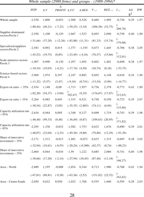
From Table 1 we can see that the sign of the parameter associated to the level of exchange rate is positive, to indicate that a devaluation reduces investments. This result is relevant and counterintuitive, as we would expect that a devaluation (reduction of REX) stimulate investment. However, in the long run a devaluation may depress investment, with an impact that varies depending on firms characteristics.
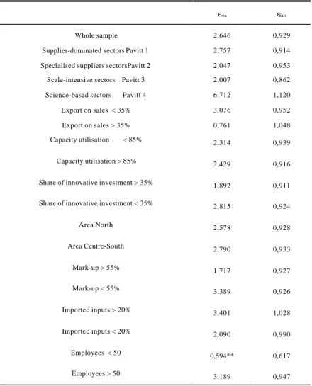
In Table 2, we show the pattern of the long run elasticities of investment with respect to exchange rate across different groups of firms.For instance, firms with a greater share of export to sales show a long run elasticity nearly one fourth smaller than the elasticity for less exporting firms. This is not surprising considering that the success in the international markets is not due to temporary competitive advantage, but to other more permanent firm characteristics, such as the accomplishment of higher standards in the product quality.
Empirical evidence in favour of such intuition can be collected by looking at the results obtained on other groups of firms , namely those grouped according to the degree of innovation embodied into investments goods, those grouped according to the degree of market power and, finally, those grouped according to the presence of a low or high foreign exposure of costs. From table 2 we see that firms with a higher share of innovative investments with respect to total investment spending are less sensitive to changes in the exchange rate, while the opposite can be observed for the less innovative firms. Again this is a symptom that
6 For the exact description of the estimation procedure see the Technical Notes
of Eviews 3.1 manual. For further details on the data employed and the computation of the variables see Appendix A.
innovative firms do not rest on temporary competitive advantage. At the same time, the group of firm with greater market power shows a weaker sensitivity to exchange rate, while the group with greater share of imported inputs (higher foreign exposure of costs), whose profits may be reduced by a devaluation, results to be more sensitive compared to that with a lower foreign cost exposure.
Broadly speaking, from estimation of the long run elasticities it seems that firms with higher mark up, greater share of innovative investment, more export oriented, with low foreign exposure of costs, higher R&D intensity and those supplying differentiated goods, are less sensitive to exchange rate variations as far as investment spending is concerned. For these firms investment decisions are weakly related to short run increment of competitiveness due to exchange rate.
We can further explore the issue of foreign exposure of cost and revenues employing the dynamic model of equation (2). In Table 3 we report our findings which are very similar to those obtained by Nucci and Pozzolo (2000).7 We can observe that variability of costs, following a devaluation, is responsible for the reduction of investment. This is because exchange rate variability reduces expected profits through the channel of imported inputs, and this effect is not offset by a similar increase in revenues. This may depend on various factors:
1) foreign exposure of costs may be greater than that of revenues. Thus a devaluation reduces profit because it
7 The estimation of equation (2) without the two foreign exposure parameters
shows that the parameter associated to ∆ rext is positive, thus supporting the
reduces the price-cost margin, as for firms that import more and export less;8
2) after a devaluation, the increase of costs is direct and quite fast, while that of revenues is indirect, with a time lag causing a sort of a J curve at firm level. Therefore, even export oriented firms may suffer from a devaluation, at least in the short run;
3) expected profits are influenced by exchange rate variability, as it introduces further uncertainty. Beyond price variability in the domestic market linked to domestic market power, firms face uncertainty due to the exchange rate volatility, which they cannot easily manage.
In the remaining part of the paper we try to shed some lights over this latter aspect, to see whether market power is the key factor in explaining investment behaviour.
3. Exchange rate volatility, expected profit and market power: a model with signal extraction problems.
From a theoretical point of view, a volatile exchange rate can offer profit opportunities to export oriented firms, provided that they behave like risk neutral agents. However, for irreversible decision, such as investment spending, and given risk neutrality, a
8
In our dataset, the group of export oriented firms show a similar foreign exposure of costs compared to that of the less export oriented ones. These latter face an increase of costs after a devaluation, but cannot easily offset it raising revenues in foreign markets. Considering that the number of firms in the two groups is nearly the same, this argument can account for the reduction of investment only if the behaviour of this group of firms prevail over the former.
greater profit volatility may reduce the optimal (desired) stock of capital in any period, depending on firm foreign exposure.9 As we stressed in the previous section, firms with greater market power can offset the negative effects of a volatile exchange rate. A firm with either a low domestic market power or acting in a more competitive international markets, has to face a higher degree of uncertainty, given that exchange rate shocks will prevent them from obtaining reliable estimates of the present value of future profit streams.
A model that wants to explain these behaviours should link investment to expected profit, assigning a role to exchange rate expectations. In that respect, a model in which firms perceive exchange rate variation as permanent, as for instance in Nucci and Pozzolo (2000) , does not seem adequate . Moreover, it is necessary to investigate how expectations take form. Failing this, all investment models based on expected profitability would neglect the uncertainty about future profit due to exchange rate and the reduction of firm growth capability. The estimations carried out until now, though in the dynamic form, leave undefined the effect of exchange rate uncertainty on investment. Hence, we need to form some hypotheses on the mechanism according to which expectations take form.
9 Hayashi (1982) underlines that, given profit defined as π
t = [pt F(Kt, Nt) – wt Nt,], where p is the firm output price, F is the production function, K is the
capital stock N is the vector of inputs and w the vector of input prices, maximising the present value of firm, under the capital accumulation constraint with adjustment costs, we obtain the identity between marginal benefits and marginal costs of a unit of capital. In this way we may define the optimal path of investment. Given the cost of an additional unit of capital, changes in the marginal benefits, due to variation of profit following the exchange rate fluctuation, cause deviations from the optimal investment path. The exchange rate, as it influences both p and w, will have an effect on investment which depends on the degree of foreign exposure of cost and revenues.
3.1 The model
Recently , Darby et Al. (1999), employing the Dixit and Pindyck (1994) model, show that exchange rate volatility may reduce investment. As a consequence of their framework, i.e. considering the invest-wait-do-not-invest decisions, they calculate the threshold values under which exchange rate volatility reduces investment. The necessary condition for investment to fall as exchange rate volatility increases depends directly on exchange rate volatility and inversely on the opportunity cost of waiting. The estimation carried out is however only loosely related to the model (Darby et Al., 1999).
In our attempt to find evidence of the impact of exchange rate uncertainty on investment we prefer to shed lights on the uncertainty-expected profits relation, and to derive a simple testable model. Our hypothesis is that profit volatility influence the marginal benefit of an additional unit of capital, and this source of uncertainty may cause unexpected change in the optimal investment path. We model this approach employing the Lucas (1973) framework of optimal decisions under signal extraction problems, where profit volatility affects investment decisions.
Expected profit for a firm selling in the domestic and in the foreign market depends on the domestic and the foreign price for firm’s good and its imported inputs. Although the signal extraction problem is generally related to prices, in our framework will be referred to profit. In fact, exchange rate variability affecting input and output foreign prices, makes total profit (foreign and domestic) more volatile . However, while in the original Lucas framework agents cannot distinguish the source of variability, in our framework we assume that firms can distinguish between the domestic and the foreign source of price variations. The signal extraction problem arises when, evaluating the present value of this volatile flow of foreign profits, firms are not able to precisely forecast exchange rate pattern.
If for simplicity, we neglect the labour market from our analysis (which should not be directly influenced by exchange rate)10, expected profit can be modelled as :
(3) Et (πt )= E t (p t) q t - E t (p t in) q t in - w t L t ,
where p and q are the good price and quantities, w is wage, L is total work force and p in and qin denote inputs price and quantities, respectively. By splitting both goods and input prices into the domestic and the foreign component and recalling that δ represent
the share of export and φ the share of imported inputs, we can
rewrite pt as:
(4) pt = (1-δ) pt,D + δ pt,F = (1-δ) pt,D + δ (pt,D / rext) .
where the D and F subscripts denote respectively the domestic and the foreign price. Similarly, for the input prices we will have: (5) ptin = (1-φ )pt,Din +φ (pt,Din /rext)
Following Lucas (1973) we assume that the expected price is a weighted average of the two components:
(6) Et(pt) = (1-δ) (1- θ) pt,D +δ θ Et-1 (pt,F) = =(1-δ) (1-θ) pt,D [1+ (δ θ / Et-1(rext )] where θ = σ2e /(σ 2 p + σ 2 e ) is the weight, σ 2 e represents the
variance of exchange rate, σ2p the variance of the price expressed
in the domestic currency and E is the expectation operator. If σ2e
is relatively large with respect to σ2p , then a signal extraction
problem arise, as profits show a volatility mainly due to that of exchange rate. The greater is the firm foreign exposure of cost and revenues, the more unpredictable are profits. The same
10
Actually recent studies show that exchange rate have significant wage and employment implication (Goldberg and Tracy, 1999).
argument applies to the price of imported inputs. Through these channels, exchange rate volatility determine the uncertainty on expected profit, but the extent and the implication of this relationship remain an empirical question.
3.2 Empirical results.
Exchange rate variability may affects export revenues and imported costs differently. In Table 4 the variability of foreign exposure of cost and revenues is displayed. In our sample of firms we found that revenues are more volatile than costs, considering both time series and the cross section average. Thus we need to verify the existence of a different impact of exchange rate volatility on profit depending on firms specific characteristics, and in particular on their market power. In Appendix B we report the estimation of the impact of exchange rate variability on profit, split in revenue and cost channels.
Having found evidence of the reduction of profit associated to
exchange rate variability,11 we introduce the exchange rate
variability12 (SIGMA) as a new variable in our dynamic equation (1). This variable is split according to foreign exposure of costs (φ) and revenues (δ). In its most general specification, equation (1) becomes:
(7 ∆ Ii,t = β0 + β1 ∆ Vi,t + β2 ∆ PROFITi,t +
+β3 ∆ UC i,t + β4 ∆ REXt + β5 Ii,t-1 + β6 Vi,t-1 + + β7 REXt-1 + β8 SIGMA t-1 δi + β9 SIGMA t-1 φi
11
See Appendix B and Table 5 for the results.
12
Estimation results from equation (7) are reported in Tables 6 and 7.
The first finding is that an increase in exchange rate volatility reduces investment spending through the profit channel. This support the idea that profit variability depresses investment. Moreover we would expect that exchange rate volatility has a different impact depending on firm’s sector and firm’s market power. More specifically SIGMA should be less important for those firm with market power, as these are able to cushion increases in the exchange rate variability, i.e. greater uncertainty on the ‘imported’ costs and ‘exported’ revenues, with an higher mark up.13
In order to account for sector heterogeneity and for firm’s market power we estimate equation (7) on four sub samples, obtained by grouping firms according to Pavitt firm classification. To understand the role played by market power we introduce slope and intercept dummies variables for firms with low and high mark up. The results are displayed in Table 7. Exchange rate variability, which is split according to foreign exposure of costs and revenues, is negative and significant for the supplier-dominated sector (Pavitt 1), for the specialised suppliers sectors (Pavitt 2) and the for the scale-intensive sectors (Pavitt 3). On the contrary, exchange rate and its variability are not significant for the science-based sector (Pavitt 4). This is an important result, as we expect that R&D intensive firms are less sensitive to exchange rate fluctuations when choosing their optimal investment path. The evidence suggests that the effect of variability on the cost side fall about 53% from Pavitt 1 to Pavitt 2, while it is similar for firms in Pavitt 2 and Pavitt 3. On the revenues side the effect slides down about 62% from Pavitt 1 to Pavitt 2 and rise about 40% from this latter to Pavitt 3.
13
From the financial point of view, firm with higher mark-up can rely on gr eater cash flows and thus they are less constrained in financing their investments.
Taking into account firms’ market power it is possible to underline other differences in firm behaviour. In the second and third row of each Pavitt group we display the estimation results using dummies for high and low market power respectively. The intercept dummy and two slope dummies account for differences of the response of SIGMA that interact separately with each of the two foreign exposure terms.
The evidence put forward the idea the effect of variability on investment is strictly linked to monopoly power, but it depends on the kind of sector. For the supplier-dominated sector high mark up firms are less sensitive to exchange rate variability than the average on the revenue side, while are more sensitive on the cost side. In the specialised suppliers sector we found that firms with monopoly power are not sensitive to exchange rate volatility, while the opposite results is found in the scale-intensive sector, where low mark up firms do not seem to respond to volatility. This may be due to the fact that, in our sample, low mark up firms import less inputs and export more output than the sample average. Therefore, they are less sensitive to the cost side and, due to higher competitive international markets, they can count on a lower mark up.
On the basis of these results, we can conclude that stability of the exchange rate may have a positive effect on the investment. This seems particularly true for firms with greater monopoly power, that can rely on a less volatile stream of future profit, and can better evaluate the marginal benefit of an additional unit of capital. This results in lower constraints in the adjustment to the optimal level of investment.
4. Concluding remarks
The empirical literature on the link between investment and exchange rate is rather scarce, probably due to the difficulties in disentangling the various effects within this link. However, such
an exercise is extremely useful both at microeconomic level, to understand the effects on firm growth, and at macroeconomic level, to understand the transmission effects of monetary policies. The estimates from a dynamic ECM model show the existence of a positive long run elasticity between investment and exchange rate. This means that a devaluation does not support investment spending as previously stated by Campa and Golberg (1999). Though in the short run profits may benefit from it, this does not imply firm growth in the long run. In particular, our calculation of long run elasticities shows that firms with higher mark up, more innovative, more export oriented, less import dependent, more R&D intensive and supplying differentiated goods are less sensitive to exchange rate changes. Moreover, long run elasticities show that firms with a higher market power are more equipped to face periods of wide exchange rate variability. On the contrary, firms more import dependent are bound to a greater profit volatility and consequently to less investment spending.
Therefore the key argument is the link exchange rate volatility-uncertainty. Even though a stable exchange rate does not allow for temporary gains following a devaluation, it eliminates a great source of uncertainty in the economic system. Profit expectations can be better evaluated by both firms and the financial system, resulting in higher confidence on investment profitability. This has been verified employing a dynamic model which takes into account profit expectations. Our results show exchange rate volatility may exacerbate that of profits, because of signal extraction problems, which in turn reduce firms forecast ability and investment spending. The decrease in investment spending is inversely proportional to firm market power.
Another important result emerging from the empirical analysis is the importance of the two channels (revenues and costs) through which exchange rate affects investment. A devaluation may increase investment provided that the effect on costs is lower than that on revenues. This depends on the degree of firm foreign
exposure and on other firm characteristics, such as its sector. According to our hypothesis, a volatile exchange rate reduces investment because it raises the difficulties related to the evaluation of marginal benefits of new capital goods. However, firms with high market power result being more sheltered with respect to this problem.
To this extent, an economic system may benefit from a stable exchange rate in terms of investment and profit, provided it is able to strengthen its firm market power.
References
Campa, J., L. Goldberg (1995), "Investment, exchange rates and external exposure", Journal of International Economics, vol. 38, n.3-4, pp. 297-320.
Campa, J., L. Goldberg (1999), "Investment, Pass-Through and
Exchange Rates: a Cross-Country Comparison",
International Economic Review, vol. 40, n. 2, May, pp.
287-314.
Darby J, Hallet A.H., Ireland J., L. Piscitelli (1999) , “The impact of exchange rate uncertainty on the level of investment”,
The Economic Journal, vol. 109, n. 2, pp 55-67.
Dixit A., R. Pindyck (1994), “Investment under uncertainty”, Princeton, Princeton University Press.
Gavin M. (1992), "Monetary Policy, Exchange Rates and Investment in a Keynesian Economy", Journal of
International Money and Finance, vol. 11, n.2, pp. 145-161
Goldberg L. (1993), "Exchange Rate and Investment in United States Industry", Review of Economics and Statistics, vol. LXXV, n. 4, November, pp. 575-588.
Goldberg L., Tracy J. (1999), “Exchange Rates and Local Labour Markets”, Federal Reserve Bank of New York, Staff Report, February, n. 63.
Hayashi F. (1982), “Tobin's Marginal q and Average q: a Neoclassical Interpretation”, Econometrica, vol.50, pp.213-224.
Lucas R. (1973), “Some International Evidence on output-inflation trade offs”, American Economic Review, vol. 63, pp.326-334.
Lucas R., E. Prescott (1971), “Investment Under Uncertainty”,
Econometrica, vol.39, pp. 658-681.
Nucci F., A.F. Pozzolo (2000), “Investment and the Exchange Rate”, European Economic Review, vol. XX, pp. 259-283.
Onida F. (1986), “Tassi di cambio, vantaggi comparati e struttura industriale”, in T. Padoa Schioppa (ed.), “Il sistema dei
cambi oggi”, Bologna, il Mulino.
Paganetto L. (1995), “Tassi di cambio, investimenti e sistema industriale italiano”, in Studi per il Cinquantenario , Ufficio Italiano Cambi, Bari-Roma, Laterza, pp.85-111.
Schiantarelli F. (1996), Financial Constraints and Investment: Methodological Issues and International Evidence, Oxford Review of Economic Policy, Summer, v. 12, iss. 2, pp. 70-89.
Appendix A – Data sources and variables description
Data Set. The data set employed in this paper is collected by
Mediocredito Centrale. The Survey of Manufacturing Firms (SMF) is carried on by the Observatory on small and medium firms, which is within the Research Department of Mediocredito Centrale. The survey was put in place for the first time in 1968, and then repeated more o less every five years until 1989. From 1989 the interval has been reduced to three years. The last three versions cover the period 1989-91, 1992-94 and 1995-97. The SFM samples firms with 11 to 500 employees and it collects information on all the firms with more than 500 employees. The sample, of about 5000 firms, has been stratified according to the number of employees and location, taking as benchmark the Census of Italian Firms.
We employ two surveys covering a period of 6 years (1989-94), with 2988 firms. The choice of period is particularly interesting because it comprises a period of wide exchange rate variability, due to the exit of lira from SME.
Firm variables. Profits Profit = Sales Costs Labour added Value − .
User cost of capital
∆ + + ⋅ = t t t t t i Pi Pi dep r Pi UC ,
where Pi is the deflator for new capital goods, dep is depreciation rate of installed physical capital, calculated with a moving average over three years of the ratio between depreciation and the book value of physical capital; r is the average interest rate on debt, calculated with a moving average over three years of the ratio between total interest paid and the sum of short and long term debts.
Mark-up mkup = 1- [( sales + ∆ inventories – intermediate inputs) / (sales + ∆inventories)]
Foreign exposure of cost and revenues.
By this term we denote the degree of firm dependence respectively on import of inputs and export sales. This latter value is reported in the survey. The foreign exposure of cost is proxied by the ratio between debt with foreign suppliers and debt with all suppliers. If firms keep stable relationship with non domestic suppliers, this measure is likely to be unbiased.
Foreign exposure of revenues
δ = export / sales
Foreign exposure of costs
φ = debt with foreign suppliers / debt with all suppliers
Macroeconomic variables Exchange rate
REX is the actual real exchange rate as calculated by Banca
d’Italia. This is the price of a bundle of foreign currencies expressed in terms of liras. Therefore a reduction of exchange rate means a devaluation of lira with respect to the currencies in the bundle.
The rate of growth is obtained by (rext - rext-1) / rext.
The exchange rate variability is calculated as the annual average standard deviation of quarterly REX.
Deflators
Sales are deflated employing GDP deflators. Investment is deflated using the investment deflator (Source Banca d’Italia).
Appendix B - The impact of exchange rate variability on profit.
The exchange rate-profit relationship may be estimated by OLS employing the following equation:
(B.1) PROFITi,t = β0 PROFIT i,t-1 +β1 rext-1 +
+β2 SIGMA t-1
where SIGMA denotes exchange rate variability14. In order to
verify the impact through the costs and revenues channels, we split exchange rate variability according to foreing exposure of costs (φ) and revenues (δ):
(B.2) PROFITi,t = β0 PROFITi,t-1 + β1 rex t-1 +
+β2 (δi SIGMA t-1) + β3 (φi SIGMA t-1)
The results are reported in Table 5. In the first row the estimate of parameters of equation (B.1) are displayed. A devaluation in the previous period increases profit, but exchange rate variability, represented by SIGMA, reduces firm profitability.15 In the second row we show the results of the estimation of equation (B.2), with
SIGMA split. We found evidence for the theoretical hypothesis
that while an increment of volatility may reduce profit through the cost channel, it may increase them through that of revenues, because a greater variability is associated to higher profit opportunities. This findings can be strengthen if we take into account firm market power. In the last two rows of Table 5 we estimate equation (B.2) introducing a dummy for mark up. Firms with higher market power are not sensitive to exchange rate
14 See appendix A for the details about the calculation of SIGMA. 15
The test on the restriction on the parameters β2=β3 = 0 in equation (A.2)
volatility through the cost channel, as they can offset a rise in the cost of imported inputs with higher mark ups. On the contrary firms with less market power seem able to profit from exchange rate variability.
Table 1 – Estimates of the dynamic investment model (ECM): equation (1)
Whole sample (2988 firms) and groups – (1989-1994)*
INTP ∆ V PROFIT∆ ∆ UC ∆ REX V t-1 REX t-1 I t-1 Ad.
R2 DW Whole sample -2,530 1,009 -0,053 -1,500 0,526 0,669 1,905 -0,720 0,39 1,97 (-80,44) (49,21) (-7,23) (-59,25) (3,16) (206,30) (32,75) (-266,76) Supplier-dominated sectors Pavitt 1 -2,550 1,108 -0,129 -1,667 1,523 0,693 2,090 -0,758 0,40 1,90 (-31,66) (37,20) (-12,26) (-82,88) (11,31) (81,33) (15,74) (-179,08) Specialised suppliers sectors Pavitt 2 -2,583 0,892 0,015 -1,377 -1,193 0,673 1,445 -0,706 0,38 2,05 (-45,52) (19,75) (0,85) (-23,49) (-4,16) (76,57) (15,86) (-112,01) Scale-intensive sectors Pavitt 3 -1,907 0,990 -0,130 -1,297 1,692 0,602 1,401 -0,698 0,38 1,97 (-10,34) (19,03) (-4,21) (-17,74) (4,50) (26,74) (8,18) (-53,75) Science-based sectors Pavitt 4 -3,969 1,974 0,297 -2,167 0,882 0,692 4,148 -0,618 0,34 1,96 (-11,32) (5,57) (3,47) (-9,10) (0,741) (13,54) (5,89) (-14,77) Export on sales < 35% -2,934 1,148 -0,08 -1,713 1,957 0,736 2,378 -0,773 0,42 1,90 (-82,20) (54,37) (-5,04) (-102,67) (9,35) (176,67) (17,07) (-212,63) Export on sales > 35% -3,264 0,982 0,045 -1,315 0,521 0,758 0,550 -0,723 0,39 2,07 (-38,54) (22,87) (3,05) (-35,35) (2,803) (74,11) (6,94) (-115,86) Capacity utilization rate
< 85% -2,610 0,944 0,005 -1,348 0,127 0,698 1,719 -0,743 0,39 1,98 (-48,48) (99,33) (0,48) (-36,49) (0,87) (109,63) (20,95)
(-171,82) Capacity utilization rate
> 85% -2,295 1,336 -0,032 -1,582 1,753 0,632 1,676 -0,690 0,39 2,01 (-40,07) (23,04) (-2,33) (-49,36) (9,88) (79,86) (12,29) (-91,29) Share of innovative investment > 35% -2,171 1,512 -0,013 -1,401 -0,072 0,633 1,315 -0,695 0,38 2,02 (-32,94) (19,61) (-0,55) (-20,24) (-0,300) (62,37) (8,74) (-88,23) Share of innovative investment < 35% -2,604 0,844 -0,034 -1,59 1,222 0,685 2,086 -0,741 0,40 1,98 (-38,66) (17,20) (-2,14) (-27,94) (10,45) (87,46) (11,18) (-166,27) Area – North -2,689 1,195 -0,088 -1,654 0,344 0,713 1,980 -0,768 0,42 1,94 (-67,01) (89,81) (-9,38) (-63,36) (2,52) (151,82) (22,52) (-242,62)
(-72,37) (19,35) (2,92) (-19,75) (6,581) (135,80) (9,52) (-77,33) Mark up > 55% -2,418 1,068 -0,054 -1,512 0,281 0,677 1,254 -0,730 0,39 2.01 (-43,57) (28,07) (-4,69) (-33,93) (1,21) (108,89) (10,33) (-169,96) Mark up < 55% -2,613 0,987 -0,066 -1,534 0,727 0,666 2,437 -0,719 0,39 1,89 (-74,14) (92,29) (-4,42) (-38,69) (3,85) (124,96) (33,86) (-123,56) Imported Inputs > 20% -3,282 1,295 -0,090 -2,089 1,308 0,782 2,735 -0,804 0,44 1,94 (-42,28) (17,02) (-2,95) (-28,97) (3,70) (77,00) (17,78) (-102,87) Imported inputs < 20% -2,904 1,161 0,053 -1,276 0,353 0,707 1,492 -0,714 0,36 2,01 (-46,94) (21,13) (2,77) (-20,00) (1,242) (71,12) (9,29) (-100,12)
Employees less than 50 -0,447 0,501 -0,051 -1,403 -0,897 0,399 0,384 -0,647 0,36 1,99 (-8,94) (8,67) (-6,03) (-33,75) (-9,22) (67,15) (1,72)
(-165,80) Employees more than
50 -2,791 1,174 -0,058 -1,556 1,355 0,713 2,401 -0,753 0,38 1,97 (-65,23) (45,78) (-8,22) (-47,67) (8,07) (162,61) (28,18)
(-289,58)
GLS estimation method for 6 years. Student’s t in brackets.
Dependent variable rate of growth of I (Investment). All regressors are in logs: Vi t
-(Sales); PROFITit (Profit), UCit (User cost of capital); REXt (real exchange rate of the
lira). The actual estimation period is 1991-1994, due to the lags and first differences in the variables.
Table 2 - Long Run elasticities: equation (1) Whole sample (2988 firms) and groups – (1989-1994)*
εrex εfatt
Whole sample 2,646 0,929
Supplier-dominated sectors Pavitt 1 2,757 0,914
Specialised suppliers sectors Pavitt 2 2,047 0,953 Scale-intensive sectors Pavitt 3 2,007 0,862 Science-based sectors Pavitt 4 6,712 1,120
Export on sales < 35% 3,076 0,952 Export on sales > 35% 0,761 1,048 Capacity utilisation < 85% 2,314 0,939
Capacity utilisation > 85% 2,429 0,916
Share of innovative investment > 35% 1,892 0,911
Share of innovative investment < 35% 2,815 0,924
Area North 2,578 0,928 Area Centre-South 2,790 0,933 Mark-up > 55% 1,717 0,927 Mark-up < 55% 3,389 0,926 Imported inputs > 20% 3,401 1,028 Imported inputs < 20% 2,090 0,990 Employees < 50 0,594** 0,617 Employees > 50 3,189 0,947
* From equation (1): εrex = –(β9 / β5), εfatt = –(β6 / β5).
Table 3 - Dynamic investment model: equation (2)
Whole sample (2988 firms) and groups – (1989-1994)*
Dependent variable: ∆ I ∆ I t-1 ∆ V ∆ REX •φ (Cost) ∆ REX •δ (Revenues ) Whole sample -0,477 0,581 8,638 -1,712 (-97,01) (10,48) (9,10) (-3,72) Supplier-dominated sectors Pavitt 1 -0,449 0,371 7,890 0,542
(-20,89) (2,19) (3,28) (0,52) Specialised suppliers sectors Pavitt 2 -0,487 0,563 8,504 -2,953
(-45,11) (3,97) (5,25) (-2,91) Scale-intensive sectors Pavitt 3 -0,395 0,513 8,929 -2,466 (-39,03) (3,12) (2,63) (-9,14)
Science-based sectors Pavitt 4 -0,694 3,390 5,272 -3,542 (-11,25) (5,73) (0,75) (-0,64) Capacity utilization rate < 85% -0,497 0,322 4,076 -0,468
(-133,40) (3,34) (2,77) (-0,74) Capacity utilization rate > 85% -0,402 1,000 10,004 -1,662
(-89,16) (10,77) (4,69) (-1,85) Share of innovative investment > 35% -0,473 0,703 5,031 -2,342 (-64,46) (6,22) (2,89) (-3,68)
Share of innovative investment < 35% -0,441 0,225 9,951 -0,334 (-34,77) (6,58) (6,29) (-0,64) Area – North -0,472 0,812 8,422 -0,074
(-46,46) (9,24) (8,16) (-0,12) Area – Centre South -0,511 -0,532 5,241 -5,466 (-13,78) (-2,28) (1,73) (-3,33)
Mark up > 55% -0,502 0,759 7,390 0,609 (-13,66) (3,02) (1,95) (0,24)
Mark up < 55% -0,472 0,476 8,948 -2,946 (-11,61) (1,51) (2,44) (-1,30) Employees < 50 -0,378 -0,024 4,875 -7,403 (-13,01) (-0,06) (1,07) (-5,14) Employees > 50 -0,507 0,613 9,616 -0,964 (-57,41) (6,66) (10,04) (-1,77)
* GLS estimation method for 6 years. Student’s t in brackets.
Dependent variable rate of growth of I (Investment). All regressors are in logs: Vit
-(Sales); REXt (real exchange rate of the lira); δ (foreign exposure of revenues); φ (foreign
exposure of costs). The actual estimation period is 1992-1994, due to the lags and first differences in the variables.
Table 4
Foreign exposure of costs and revenues: standard deviation
Years Foreign exposure of costs φ Foreign exposure of revenues δ 1990 0.0108 0.0160 1991 0.0019 0.0029 1992 0.0026 0.0039 1993 0.0237 0.0352 1994 0.0047 0.0070 Cross-section average 0.0178 0.0286
Table 5
Exchange rate variability and Profits Whole sample (2988 firms) – (1989-1994)*
PROFIT (t-1)
rex SIGMA SIGMA ⋅ δ SIGMA ⋅φ Dummy high markup Dummy low markup Slope dummy SIGMA⋅ δ Slope dummy SIGMA⋅ φ Ad. R 2 DW (1) 0,912 -1,517 -0,011 0,33 2,48 (766,8) (-59,70) (-3,93) (2) 0,903 -1,781 0,064 -0,048 0,31 2,47 (1069) (-73,77) (7,60) (-4,14) (3) 0,924 -1,091 -0,083 0,094 -0,002 0,32 2,50 (398,8) (-24,6) (-13,54) (8,40) (-0,13) (4) 0,928 -1,112 -0,097 0,130 0,039 0,32 2,50 (349,48) (-24,81) (-16,43) (11,78) (2,45)
* GLS estimation method for 6 years. Student’s t in brackets.
Dependent variable log PROFIT (Profit): REXt (real exchange rate of the lira); SIGMA
(standard deviation of REX); δ (foreign exposure of revenues); φ (foreign exposure of
costs). The actual estimation period is 1990-1994, due to the lags and first differences in the variables. all regressors are in logs.
Table 6
Estimates of the dynamic investment model (ECM) with exchange rate variability
Whole sample (2988 firms) – (1989-1994)*
INTP ∆V ∆PROFIT ∆ UC ∆ REX Vt-1 REXt-1 It-1 SIGMA Ad. R 2 DW -2,372 1,00 -0,034 -1,595 -3,913 0,654 1,779 -0,705 -0,366 0,40 1,90
(-104,1) (88,8) (-5,40) (-174,5) (-22,79) (288,3) (41,98) (-911,1) (-68,19)
* GLS estimation method for 6 years. Student’s t in brackets.
Dependent variable is the rate of growth of I (Investment). All regressors are in logs: Vit- (Sales); PROFITit (Profit), UCit (User cost of capital); REXt (real exchange rate of the lira); SIGMA (standard deviation of REX). The actual estimation period is 1990-1994, due to the lags and first differences in the variables.
Table 7
Estimates of the dynamic investment model (ECM) with exchange rate variability and interaction with market power
Whole sample (2988 firms) and Pavitt groups – (1989-1994) INTP ∆ V ∆UC ∆REX REX t-1 Vt-1 It-1 SIGMA
• φ SIGMA • δ Slope dummy SIGMA • φ Slope dummy SIGMA • δ Dummy High markup Dummy low markup Ad. R 2 DW Pavitt 1 -3,44 1,22 -2,08 -1,17 2,43 0,74 -0,76 -0,15 -0,08 - - - - 0,44 2,04 high mkup -3,13 1,12 -1,98 0,76 2,03 0,75 -0,77 - - -0,14 -0,06 -0,003* - 0,44 2,07 low mkup -2,82 1,24 -2,01 0,72 2,57 0,73 -0,77 - - -0,12 -0,08 -0,44 0,44 2,06 Pavitt 2 -3,46 1,001 -1,50 -1,61 1,61 0,76 -0,74 -0,07 -0,03 - - - - 0,41 2,00 high mkup -3,29 1,05 -1,54 -1,10 2,09 0,76 -0,75 - - -0,05* -0,03* -0,12 - 0,41 1,99 low mkup -3,34 0,96 -1,47 -0,86 1,74 0,77 -0,76 -0,05 -0,03 -0,06* 0,41 1,97 Pavitt 3 -2,38 0,83 -0,78 0,92 1,00 0,69 -0,79 -0,06 -0,05 - - - - 0,42 1,55 high mkup -2,44 0,81 -0,83 1,12 1,05 0,72 -0,82 - - -0,07 -0,11 -0,04* - 0,42 1,50 low mkup -2,00 0,83 -0,79 2,27 1,16 0,70 -0,82 - - -0,02* -0,01* - -0,14 0,41 1,53 Pavitt 4 -6,00 2,19 -2,65 1,23* 2,03* 1,05 -0,87 0,01* 0,02* - - - - 0,44 1,34 high mkup -6,16 2,42 -2,65 0,79* 2,14* 1,03 -0,85 - - -0,08* 0,08 0,24* - 0,44 1,39 low mkup -5,46 2,32 -2,78 -0,53* 2,13* 0,98 -0,83 - - 0,06* -0,14* - -0,22 0,44 1,39
GLS estimation method for 6 years. Student’s t are not reported.
Dependent variable rate of growth of I. All regressors are in logs: Vit- (Sales);
PROFITit (Profits), UCit (User cost of capital); REXt (real exchange rate of the lira);
SIGMA (standard deviation of REX); δ (foreign exposure of revenues); φ (foreign