SCUOLA
DOTTORALE
IN
GEOLOGIA
DELL’AMBIENTE
E
DELLE
RISORSE
XXIII CICLO
APPLICATION
OF
THE
MODFLOW
GROUNDWATER
NUMERICAL
MODEL
TO
HYDROGEOLOGICAL
VOLCANIC
UNITS
Sara Taviani
A.A. 2010/2011
Tutor: Prof. Giuseppe Capelli
APPLICATION OF THE MODFLOW GROUNDWATER
NUMERICAL
MODEL
TO
HYDROGEOLOGICAL
VOLCANIC UNITS
Tutor: prof. Giuseppe Capelli* Dottoranda: Sara Taviani
Co-tutors: Hans Jorgen Henriksen** Carlo Rosa***
* Laboratorio di Idrogeologia Numerica e Quantitativa, Dipartimento Scienze Geologiche, Univer-sità Roma Tre
** Geological Survey of Denmark and Greenland (GEUS), Copenhagen, Danimarca ***Fondazione Ing. Carlo Maurilio Lerici, Politecnico di Milano
a Cesare, curioso per le mie idee, mai banale nelle sue obiezioni ed a Giusi, pronta nel trovare il bello della vita…papà e mamma
APPLICATIONS
OF
NUMERICAL
GROUNDWATERS
FLOW MODELS TO HYDROGEOLOGICAL
VOLCANIC
UNITS ... 6
1. INTRODUCTION AND STUDY OBJECTIVES
... 6
2.
STUDY AREA
... 8
2.1CONTEXT OF SABATINI VOLCANIC COMPLEX...8
2.1.1 Geographical setting...8
2.1.2 Climate and hydrology...10
2.1.2.1 Recharge 13
2.1.2.2 Bracciano Lake 17
2.2GEOLOGICAL SETTING...23
2. 2.1 Pre.volcanic period...23
2.2.2 Volcanic period...24
2.3HYDROGEOLOGICAL SETTING- DEVELOPMENT OF THE CONCEPTUAL MODEL...27
2.3.1 Reconstruction of hydraulic discontinuity surface...33
2.3.2 Water table reconstruction and groundwater flow analysis...37
2.3.3 Withdrawal...50
2.3.4 Water budget...53
3. HYDROGEOLOGICAL MODEL... 57
3.1GOVERNING EQUATIONS...57
3.1.1 Darcy's Law ...57
3.1.2 Groundwater flow equation ...59
3.1.3 Solving groundwater flow equation ...60
3.2GROUNDWATER MODELS...62
3.2.1 General properties of gridded methods ...64
3.2.2 Modelling protocol...66
3.2.3 Conceptual model ...69
3.2.4 Boundary Conditions ...72
3.2.5 Modelling lake systems, Lake-aquifer interaction ...72
3.2.5 Code selection...77
3.2.6 Calibration process...78
3.2.6.1 Parameter ESTimation (PEST) 80
3.2.6.2 Sensitivity analysis 83
3.2.7 Model verification...84
4. CONSTRUCTION OF BRACCIANO MODEL
... 85
4.2HYDRAULIC PARAMETERS...85
4.3MODEL BOUNDARY CONDITIONS...86
4.4BRACCIANO LAKE...88
4.5 RECHARGE...90
4.6 WITHDRAWAL...91
4.7 SELECTION OF CALIBRATION TARGETS...92
4.7.1 Uncertainty Determination ...93
4.7.2 Numerical criteria...98
5. CALIBRATION
... 101
5.1VMFBRACCIANO MODEL CALIBRATION AND TENTATIVE VALIDATION...101
5.1.1VMF Bracciano model, steps followed ...101
5.1.2 Tentative model validation...110
5.2GWVBRACCIANO MODEL CALIBRATION...113
5.2.1 Two layer starting model ...113
5.2.2 Selection of calibration targets...114
5.2.3 Overview of the main steps followed...115
5.2.4 Model A...115
5.2.5 MODEL B ...119
5.2.6 Model C...125
5.2.7 Model D...128
5.2.8 Discussion ...129
6. MODEL DISCUSSION AND CONCLUSIONS
... 132
8. BIBLIOGRAPHY
... 137
9. ACKNOWLEDGEMENTS... E
RRORE
.
I
L SEGNALIBRO NON È
DEFINITO
.
A.1
APPENDIX A: DETAILED GEOLOGIC SEQUENCE
... 145
A1.1 PREVULCANIC STRATIGRAPHIC SEQUENCE...145
A1.2 VOLCANICUNITS...146
A.2 ANNEX B: TABLES RELATIVES TO ALL THE GAUGING
STATIONS PRESENTED IN THE AREA OF STUDY
... 159
APPLICATIONS
OF
NUMERICAL
GROUNDWATERS
FLOW
MODELS
TO
HYDROGEOLOGICAL
VOLCANIC
UNITS
1.
I
NTRODUCTION AND STUDY OBJECTIVESThis study is part of “multi step collaboration” between the Regional Groundwater Department (Autorità dei Bacini Regionali), the Regional Environmental Department (Assessorato all’Ambiente Regionale) and the University of Roma Tre. The aim of the projects overtaken in the last fifteen years has been the evaluation of the water resources.
Defining the study objectives is an important step in applying a ground water flow model. The ob-jectives aid in determining the level of detail and accurancy required in the model simulation. Complete and detailed objectives would ideally be specified prior to any modelling activities. (ASTM, D5447-04)
The objectives of this work of study are:
To build a Bracciano conceptual model that could “contain” all the achieved information and analy-sis about a complex context. A conceptual model at basin scale (380 km2), that could on one side take in consideration all the complexities of the Bracciano volcanic deposits and on the other side that could arrive to a simplify representation. Bracciano hydrogeologic basin include: four caldera structures, two of these still occupied by lakes. There are two big withdrawal sites: one from lake and the other fed by drains on the northwest side of the Lake Bracciano. At the same time the area is exposed to a continuous exploitation and dewatering from effect of the several public and private pumping wells put in action in the last twenty years. Considering the Lake Bracciano relevance (since roman period Bracciano area constituted a water reservoir for the near city of Rome) the con-ceptual model should be focused on the lake-aquifer interactions.
To build a numerical groundwater model for the Bracciano hydrogeologic basin. By use of MODFLOW, set up a site specific regional groundwater model, which could be representative of the studied context at the scale decided. The mathematical model should be coherent with the con-ceptual model elaborated and it should be a constant critical reviewing of the mathematical model and then in consequences of the conceptual model to point to a better fit between them.
To construct a regional numerical groundwater flow whereby all the data and geological interpreta-tions can be put together allowing quantitative evaluainterpreta-tions of groundwater recharge, water balance for the lake and the aquifers. The idea with the numerical model is to try to evaluate whether the conceptual model can be confirmed by simulations and validation tests using data not used for cali-bration. Part of this objective is to find out how the conceptual model can be translated into a nu-merical model (simplified etc.), how boundary conditions can be introduced in the MODFLOW setup, rivers, drains, pumping wells, discretization, parameter zoning etc.
Further objective is to assess whether and to what extent the numerical modelling can be a powerful aid in the management of water resources for predictive simulations. It can be a powerful aid for different reasons. It can give feedback to data collection, conceptual model, process understanding, geological interpretation. It is a quantitative way of understanding groundwater levels and flow rela-tionships. It can give input to local models etc.
It is important to understand if it is possible always think to use numerical hydrological modelling for management purposes and under what conditions. And if is not possible, which claims to give. Setting of a monitoring network could be of help in the improving of a model site building and in the validation of the model, necessary step for model that could be used with a predictive approach.
2.
STUDY AREA2.1CONTEXT OF SABATINI VOLCANIC COMPLEX 2.1.1 Geographical setting
The region of Sabatini complex covers an area larger than 1690 km2 and it is located in the northern area of Rome (Central Italy). The volcanic activity conditions the morphological structure of the overall area.
The products of more distant volcanic activity belonging to the Vicano and Cimino complexes par-tially cover the northernmost part of this geographical area.
The study area belong to the Sabatini complex and it is constituted by the hydrogeologic basin of Bracciano Lake 380 km2 wide. Baccano, Polline, Stracciacappe, Martignano and Bracciano depres-sions are part of it (see Fig. 2.1).
Bracciano depression is the largest one (about 380 km2) and it was caused by a volcano-tectonic collapse. Other lower surface areas are presents, identified as small craters or calderas.
The depressions of Bracciano, Martignano and Monte Rosi are occupied by lakes, Their altitudes above sea level (a.s.l.) are 162, 205 and 237 m.and their depth 160, 54 and 5 m, respectively.
Until the 19th century some calderas were filled with water: there was a lake basin in the Straccia-cappa caldera depression, drained by a tunnel connected to Bracciano Lake where another tunnel draining from Martignano joined; in the depression of Baccano caldera there was a swamp, drained by a tunnel in the south-southeast side of the valley.
Baccano valley is also open to the East and is connected to the Tevere River by the Curzio stream. Aforementioned depressions are usually surrounded by a series of asymmetric topographic profile relieves with steep slopes inwards and more gentle slopes outwards.
In the northwest part, these depressions are surrounded by relieves: Rocca Romana (612 m a.s.l.), M. Raschio (554 m a.s.l), Monte Calvario (541 m a.s.l) and Poggio delle Forche (530 m a.s.l).
Figure 2.1: Topographic map of the study area
The relief, delimiting the Bracciano depression, has an opening at southeast (near Anguillara vil-lage) from which the lake effluent Arrone river originates.
In the east and southeast side the hills slope downwards to the Tevere valley and to the sea.
Some ridges develop radially towards the northeast, east and south, while numerous incisions, with valleys very close to each other and steep walls, generate a particular landscape characterized by young morphology and ongoing erosion.
Bracciano lake north perimeter relief is linked to Vicani relief.
The Tevere valley and the coastal plains has a completely different morphology with maximum heights of a few tens of meters with deep incisions.
2.1.2 Climate and hydrology
In this region the most important aspect of the climate is the peculiar precipitation regime. Precipi-tations (generally more than 900 mm/year) are usually concentrated in a restricted period of the year lasting between autumn and spring. They often occur in intervals of more consecutive days. Severe event are common. As a consequence, terrains soon reach saturation and generate runoff, main ero-sion contribution. The drainage pattern is generally radial towards the lake and with higher intensity in the south.
To summarize, severe erosion, affecting the river-beds on the volcanic edifice, is casued by three main concomitant factors: a) precipitation regime; b) high relief; c) lithologic heterogeneity.
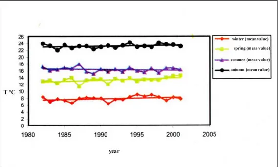
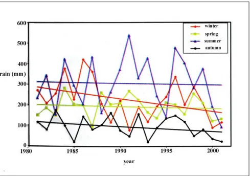
In the period 1980-2000 observations at the SIMN (Serivizio Idrografico e Mareografico Nazionale) gauging stations showed an increase of annual mean temperature and a decrease of the annual pre-cipitation (around 150-200 mm in 20 years) as shown in Fig. 2.2 and Fig. 2.3 (Capelli et al., 2005). Consequently, the impact of reduced rainfall and effective infiltration is not proportional to the av-erage annual values, but depends on the combination of seasonal factors. For instance, the reduction of winter precipitation reduces the water supply in the period when evapotranspiration is minimal, thus introducing a net loss of effective infiltration. On the contrary, the availability of water in the warmer period results in increased evapotranspiration (see below). Similarly, the greatest tempera-ture variations were in spring, when evapotranspiration reaches its maximum values.
Figure 2.2: Seasonal temperature trend recorded by SIMN stations between 1980 and 2000 and relative re-gression curves.
Figure 2.3: Seasonal rainfall trend recorded at SIMN stations between 1980 and 2000 and related regression curves.
The above considerations stress the need and the importance to examine the budget on monthly ba-sis, ideally even daily, to take into account the climate factors variability during different years. The hydrologic budget analysis also requires spatial extent for the abovementioned factors. Hence rainfall and temperature spatial reconstruction were needed.
Daily minimum, maximum and average temperature values and recorded rain by meteorological stations have been monthly aggregate and expressed as average value for the temperature and cu-mulative value for the rain measurements.
It was build a special macro to obtain cumulative rainfall and mean temperature by establishing cri-terion for the malfunctioning stations. It was defined a maximum number of days of not function-ing, beyond which the monthly information was not considered for a specific station.
The hydrologic annual balance was analyzed on a monthly basis calculated from daily values, so it was possible to take into account the variability inside the year. The recharge has been calculated starting from the monthly estimate on cells 250x250 meters on two periods (1997 -2001 and 2002- 2008), of the following parameters:
- Rainfall;
- Maximum temperature; - Mean temperature; - Minimum temperature.
The geostatistical method Random Function of K Order (IRFk) kriging (Chilès & Delfiner, 1999; Wakernagel, 1995; Bruno e Raspa, 1994; Matheron, 1973), which is valid in not-steady conditions, was applied to produce a set of maps describing parameters distribution;
The accuracy of the estimation is based on processes and data statistics derived from cross-validation by comparison with measured values. The cross-cross-validation has been performed for all 4 parameters at each observation point and month (12 months for 5 years, 60 in total). After comple-tion of cross-validacomple-tion process, the variance of the relative errors has been calculated to assess the quality of the generated monthly maps.
The variance of rainfall is lower in the period 2000-2001 than 1997-99 (Fig. 2.4). Figure 2.5 indi-cates the frequency distribution of the relative standard deviation of the cross-validation errors. The value is lower than 0.5 for more than 80% of the cases and lower than 0.3 for 50% of the cases (months).
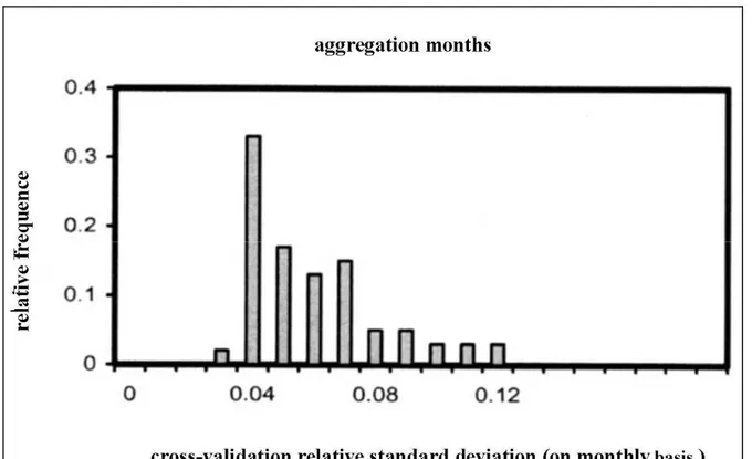
Figure 2.5: Histogram of cross-validation relative standard deviation (on monthly basis) of monthly precipi-tation in the period 1997-2001
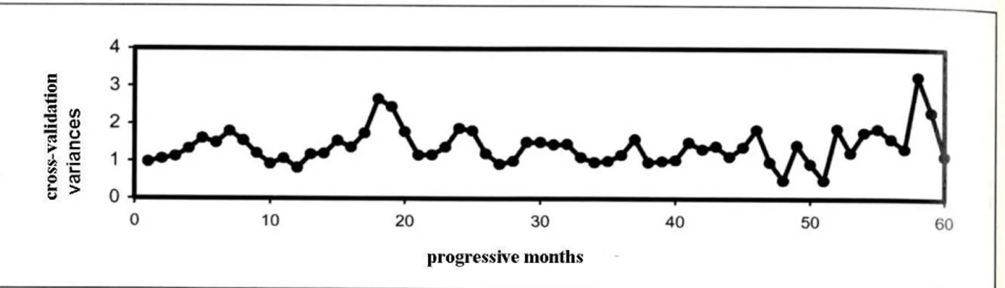
Temperature cross-validation variance, excluding few months, oscillates between 1 and 2°C (Fig. 2.7). The frequency distribution of the relative standard deviation of cross-validation (Fig. 2.6) shows values ranging between 0.01 and 0.12. In 50% of the cases, values is lower than 0.05 and in 83% of the cases is lower than 0.08
The cross-validation was performed taking into account the estimation point elevation above the sea level to eliminate systematic errors otherwise introduced.
Figure 2.6: Histogram of cross-validation relative standard deviation (on monthly basis) of maximum tem-perature in the period 1997-2001
Figure 2.7 – Temporal trend of cross-validation variance of maximum monthly temperature in the period 1997-2001.
Figure 2.8 shows rainfall trend (for the years from 2000 to 2006) at 8 rain gauge stations present in the area (telemetric: Baccano, Bracciano, Castello Vici, Cerveteri, Formello, La Storta; automatic: Tragliatella and Trevignano Romano). There are periods without data due to malfunctioning of the instruments. The data were analyzed for the period 1951-2007, but measurements later than 2003 have not yet been validates by National Hydrographic Service (Servizio Idrografico Nazionale).
0 50 100 150 200 250 300 350 400 450 500 2000 2001 2002 2003 2004 2005 2006 year r (mm /m ont h ) CERVETERI TRAGLIATELLA
BRACCIANO CASTELLO VICI
FORMELLO LA STORTA ACEA
TREVIGNANO ROMANO
Figure 2.8: Rainfall patterns in the study area
2.1.2.1 Recharge
The recharge is represented by a raster map (250 x250 m cells) with each cell representing the cor-responding calculated recharge. The recharge has been calculated using the “method of distribute
balance” as reported by Capelli et al.(2005). The annual recharge in each cell is the difference be-tween precipitation, runoff and real evapotranspiration.
The effective infiltration is the portion of rain that contributes to aquifer recharge. In the case of aq-uifers where contributions of surface water and groundwater from adjacent areas can be considered as negligible, the effective infiltration corresponds to the amount of renewable resource, and thus available for the maintenance of underground and surface outflow/inflow basis of the waterways and for human activities.
In different areas of the hydrological basin, the recharge has different values according to:
- climate spatial and temporal distribution (temperature, rainfall, solar radiation, wind speed, humid-ity);
- morphology (slope, exposure, presence of drainage areas and/or semi-endorheic areas - aquifer lithology (rock permeability);
- soil characteristics (available water capacity (AWC), effective porosity, etc.); - vegetation cover and land use ;
The maximum size of computational cells must be comparable with the minimum size of consid-ered cartographic elements (land use, lithological associations, morphology, AWC, etc.).
The timescale should allow to consider seasonal variability and, ultimately, distribution and inten-sity of meteorological events. The experimental data currently available made necessary monthly, in some case even daily, approach. It is always advisable to obtain the recharge as the sum of monthly or daily contributions, in order to take into account variability of regional and climate factors during several years.
In Table 2.1 is represented a scheme of the process of recharge calculation including the estimation of the main variables (temperatures, precipitation, runoff).
Table 2.1: scheme for calculating the distributed value of recharge
starting data kinds of aggregation - other info data processing
unit of measurement & maximum & minimun value output time depen-dent
Daily precipitation monthly cumulate precipitation
kriging, FAI-k mm P distribuited value of monthly
precipitation (grid)
yes Maximum daily temperature Tmax monthly mean of
the maximum daily temperature
kriging FAI-k, with external drift
°C Tmax distribuited value of the monthly mean of the maximum
daily temperature (grid)
yes
Minimum daily temperature Tmin monthly mean of the minimum daily
temperature
kriging FAI-k, with external drift
°C Tmin distribuited value of the monthly mean of the minimum
daily temperature (grid)
yes
Mean daily temperature (obtained by the mean of the minimum and maximum daily temperature
values)
Tmean monthly mean of the medium daily
temperatures
kriging FAI-k, with external drift
°C Tmean distribuited value of the monthly mean of the medium daily temperatures
(grid)
yes
Corine land cover (shape poligon) build specific legend
correlate to fotointerpretation areas
colors ortophotos - scale 1:10.000 Regione Lazio flight 2000
fotointerpretation of colors ortophotos
topographic map 1:10.000 draw perimeters UTW
H=thickness of soil (m) -from geology map (1:25.000) poligon.shp P= gradient of stone (%) 120=mean unitary value of AWC for the
considered soil (mm/y) F=correction factor for vulcanic soil
UTW(Unity of Territory Water Requirement) a monthly value of kc is associated to every UTW
class
from 0 to 1,1 Kc -distribuited monthly value of the crop coefficent (grid)
yes
hydraulic conductivity (geology) topography slope (DEM)
vegetal covering (UTW)
RA solar radiation, it has an unic monthly value for the entire area
EVR (evapotraspiration)
EVR= ETR (if there isn't deficit)
if P+Ui>ETR ETR= ETP*kc DF deficit
EVR= P+ Ui (if there is deficit)
if P+Ui<ETR
Surface Runoff Recharge
from 0 to 1
UTW (Unit of Territory Hydro exigency) mapping
units with homogeneous water requirement ( poligon)
yes
no mm, from 0 to 235 distribuited value of the AWC
(grid)
R (year)= Σ (Pmonth- EVR month- SRmonth + Endo month) SR(year) = Σ (Pmonth-EVRmonth)*Ck
Value necessary in the estimation of the Evapotraspiration
AWC= H*(1-P)*120 F Avaiable water capacity
assigning a percent value to each component
Uim = (P- ETR+Ui)m-1; if Uim>AWC => Uim=AWC; if Uim<AWC=> Uim=Uim and DF= (Ui-ETR+P)m
almost no
ETP= 0,0023 (Tmean+17,8) (Tmax-Tmin)0,5 RA
Ck -distribuited value of the
Kennessey coefficent (grid)
Surface runoff: expressed as the sum of monthly difference between precipitation and evapotran-spiration, multiplied by the average annual runoff coefficient (Kennessey coefficient, Ck) (See
Ta-ble 2.1 for the formula). The coefficient Ck has been calculated from the distributed balance given for a defined area and it is the sum of three factors changing according to the permeability of the outcropping rocks or terrains, the land cover and the surface slope. The coefficient is calculated tak-ing also into account the aridity index (Ia), which relates the annual average temperature and rain-fall to the driest month temperature and rainrain-fall. Ck is yearly valid, therefore in the hydrologic bal-ance the annual sum and not the monthly value is considered. In this way, Ck doesn’t take into ac-count the rainfall intensity distribution, introducing an error in runoff value estimation.
For instance, in the case of very intense rainfall, the evapotranspiration and the infiltration are neg-ligible respect to the runoff but, being the daily precipitation averaged on the entire month, the Ck value is underestimated.
In urban areas, the surface runoff is larger compared to the not urbanized areas, with values higher than 270 mm/yr. During runoff model calibration, monthly and annual calculated runoff has been compared with the field data collected at SIMN measurement stations in Bracciano area. The gaug-ing stations are on a limited number of streams and rivers, hence there are relevant lacks of data. However, the difference between simulated and observed values around 5% of the rainfall value on a single hydrographic basin.
During the past years experimental data have been collected (Gasparri, 1987 and Tarantino, 1991) in an adjacent basin to the study area (Cinque Bottini basin) similar to Bracciano basin from a geo-logic point of view.
Calibrated instruments were installed for flow measurement on a closed section of a watercourse. From the recorded data it was possible to distinguish runoff flow from the baseflow.
During the period 1984-1985 the mean calculated runoff was 94 mm, while in the period 1986-1987 was 55 mm.
The distributed recharge was calculated, not considering the lakes present in the study area (see Section 2.1.2.2 for the lake area). In Fig. 2.9 and 2.10 the visualization of the recharge for the peri-ods 2001 and 2002-2008. Mean recharge is 378 mm for 2002-2008 and 283 mm for 1997-2001.
Figure 2.9: Distributed recharge (m) for the period 1997-2001
Figure 2.10: Distributed recharge (m) for the period 2002-20008. 2.1.2.2 Lakes
i) Bracciano Lake
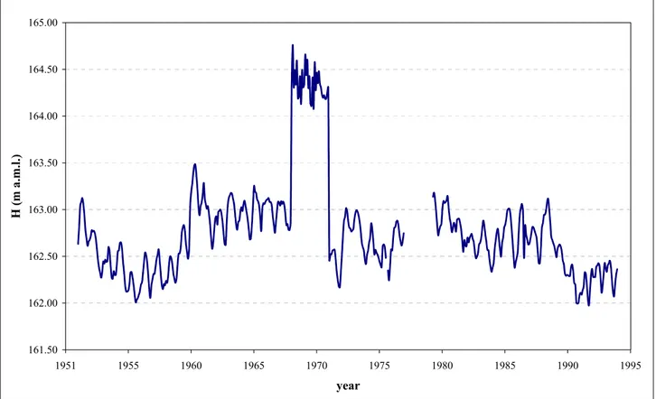
Bracciano Lake represents a very important hydrogeologic unit. It occupies about one sixth of the study area (57 km2) with a maximum depth of 160 meters and a total volume about 484.78 m3. Bracciano Lake has a direct exchange with the volcanic aquifer. Lake level are available since 1952 until today (SIMN gauging stations). Figure 2.11 and Figure 2.12 evidence that lake level is almost stable, except the period from 1969 to 1971, where sudden level raise was recorded due to malfunc-tioning of the gauge stations. In the years 1978 and 1979 some gaps were recorded due to
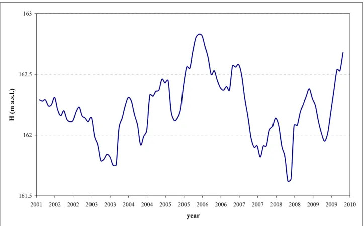
interrup-tion of data recording. It can be observed that until 1989 the level of 163 m has been exceeded sev-eral times and the lower limit of 162 m has never been reached, while from 2002 to 2010 the upper limit never exceeded 163 m and several times the lower limit went below 162 m.. level, it is possi-ble to observe a decreasing general trend.
From 1952 until 1994 the Anguillara Sabazia hydrometric station was operating and measured the lake level with a hydrometric zero of 161.74 m a.s.l. From 1995 this station was no longer working and Castello Vici hydrometric station, managed by ACEA Water Company, was operating with a different hydrometric zero corresponding to 161.79 m a.s.l, as considered in the below Figures. In 2008 the Hydrometric Regional Service installed a survey piezometer near the old Anguillara Saba-zia station, but after a while it revealed a problem, due to the interference produced by a nearby pri-vate pumping well, as a consequence information relative to this piezometer were not considered.
161.50 162.00 162.50 163.00 163.50 164.00 164.50 165.00 1951 1955 1960 1965 1970 1975 1980 1985 1990 1995 year H (m a .m.l.)
Figure 2.11: Hydrometric level of Bracciano Lake, monthly measurement values from National Hydro-graphic Service (Servizio Idrografico), from 1951 until 1994.
161.5 162 162.5 163 2001 2002 2002 2003 2003 2004 2004 2005 2005 2006 2006 2007 2007 2008 2008 2009 2009 2010 year H (m a .s .l. )
Figure 2.12: Hydrometric level of Bracciano Lake, measurement values from ACEA (Mucicipal Agency Electricity and Water), from 2001 until 2010.
Considering three SIMN gauging stations located around Bracciano Lake, the Vicentini formula was used to calculate the Evaporation on the lake:
( )
t T( )
t[
U( )
t]
E =5.33∗ +0.75100− [mm/y] Eq. 2.1
Where
T(t) is monthly average temperature U(t) is monthly average humidity
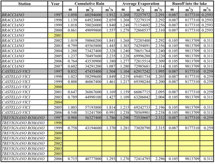
Figure 2.13 shows the location of the gauging stations. In Table 2.2 annual cumulative rain, annual average evaporation and annual cumulative runoff, calculated from monthly values, are reported. The difference between rain and evaporation is almost always negative, evidencing the prevalent role of the evaporation on the rain in the lake. Runoff value is not sufficient to restore the balance and it must therefore be assumed a component to lake recharge from the aquifer.
Table 2.2: Annual cumulative rain, annual average evaporation and annual cumulative runoff at three SIMN gauging stations. Station Year m m3/y m3/s m m3/y m3/s m m3/y m3/s BRACCIANO 1997 1.058 60294600 1.912 1.268 72257972 2.291 0.087 8177310 0.2593 BRACCIANO 1998 1.139 64923000 2.059 1.268 72279319 2.292 0.087 8177310 0.2593 BRACCIANO 1999 1.018 58026000 1.840 1.248 71154692 2.256 0.087 8177310 0.2593 BRACCIANO 2000 0.861 49099800 1.557 1.278 72860537 2.310 0.087 8177310 0.2593 BRACCIANO 2001 BRACCIANO 2002 1.019 58060200 1.841 1.268 72285400 2.292 0.105 9813709 0.311 BRACCIANO 2003 0.799 45565800 1.445 1.303 74294891 2.356 0.105 9813709 0.311 BRACCIANO 2004 1.288 73427400 2.328 1.240 70651764 2.240 0.105 9813709 0.311 BRACCIANO 2005 1.237 70497600 2.235 1.228 69996288 2.220 0.105 9813709 0.311 BRACCIANO 2006 0.764 43530900 1.380 1.277 72815514 2.309 0.105 9813709 0.311 BRACCIANO 2007 0.602 34291200 1.087 1.280 72985681 2.314 0.105 9813709 0.311 CASTELLO VICI 1997 0.832 47435400 1.504 1.104 62917242 1.995 0.087 8177310 0.259 CASTELLO VICI 1998 1.023 58299600 1.849 1.219 69481734 2.203 0.087 8177310 0.259 CASTELLO VICI 1999 0.808 46067400 1.461 1.217 69390244 2.200 0.087 8177310 0.259 CASTELLO VICI 2000 CASTELLO VICI 2001 0.647 36867600 1.169 1.159 66067715 2.095 0.087 8177310 0.259 CASTELLO VICI 2003 0.789 44990100 1.427 1.109 63206042 2.004 0.105 9813709 0.311 CASTELLO VICI 2004 CASTELLO VICI 2005 1.003 57193800 1.814 1.215 69242733 2.196 0.105 9813709 0.311 CASTELLO VICI 2006 0.548 31241700 0.991 1.238 70569901 2.238 0.105 9813709 0.311 TREVIGNANO ROMANO 1997 0.988 56327400 1.786 1.290 73530607 2.332 0.087 8177310 0.259 TREVIGNANO ROMANO 1998 TREVIGNANO ROMANO 1999 0.758 43194600 1.370 1.281 73020790 2.315 0.087 8177310 0.259 TREVIGNANO ROMANO 2000 TREVIGNANO ROMANO 2001 TREVIGNANO ROMANO 2002 TREVIGNANO ROMANO 2003 TREVIGNANO ROMANO 2005 TREVIGNANO ROMANO 2006 0.715 40777800 1.293 1.270 72414795 2.296 0.105 9813709 0.311
Cumulative Rain Average Evaporation Runoff into the lake
Lake Bracciano constituted an important water reservoir for the city of Roma, from the nineteenth century the Municipal Water Agency of Roma (ACEA) obtained the concession to withdrawal from Bracciano lake an amount of around 1000 l/s of water., that fed the Paolo aqueduct. The monthly average values of abstraction were transmitted by ACEA, for the last ten years; in Fig. 2.14 is pos-sible to see the average annual trend plot from the year 1997 to 2007 (l/s).
Withdrawal from Lake Bracciano (ACEA) 0 200 400 600 800 1000 1200 1996 1998 2000 2002 2004 2006 2008 year l/s Figure 2.14: average year value of Lake Bracciano withdrawal
ii) Martignano Lake
Martignagno Lake is a shallow smaller lake located at 2 km to the east of Bracciano with an exten-sion of 2.4 km2, water table elevation around 207 m a.s.l., maximum depth of 55 m, The lake con-sists in a close basin fed by rainfall without emissaries. During recent years the water table stood several meters (about 20) below the tunnel that fed the Roman Alsietino Aqueduct. There was an artificial outlet built in the IX century connecting the actual lake and former lake Stracciacappa (see Fig. 2.13), with Paolo aqueduct, but nowadays has been probably blocked by some collapse. Due to the absence of tributaries, the lake level has minor change and residence time is quite long, indi-cated as 29.6 years, with high risk for pollution. Martignano Lake is linked to a shallow aquifer, it was not consider in the groundwater model construction, where the focus went to the main volcanic aquifer.
2.2GEOLOGICAL SETTING 2. 2.1 Pre.volcanic period
Below the volcanic products there are autochthonous Neogene sediments lying on allochthonous deposits belonging to "Flysch tolfetani” (Fazzini et al., 1972). The Neogene sediments are in con-tact with limestone and limestone-marl of Meso-Cenozoic sequence belonging to Umbria-Marche basin (Funiciello & Parotto, 1978). Just south east of Bracciano Lake, in the area of Baccano-Cesano, the Meso-Cenozoic substratum is raised to form a small median ridge (high structural Bac-cano-Cesano) (Funiciello et al., 1979; De Rita et al., 1983; Di Filippo & Toro 1993).
2.2.2 Volcanic period
Bracciano Lake is part of Sabatini Volcanic District, which started its activity over 600,000 and ends approximately 40,000 years ago (De Rita 1993), at the same time with the other alkaline potas-sic districts in the Latium region (Central Italy). The various explosive eruption centers in the Dis-trict are in a vast area, more or less flat, largely occupied by clayey sediments of Plio-Pleistocene (Graben area of the principal Graben), limited to the west by the flysch hills of Monti della Tolfa Districts and the dominant Cerite-Manziana acid-Tolfetano with older activity. To the east the vast area is connected to the Meso-Cenozoic sedimentary hills of Mount Soratte and, further south, Monti Cornicolani. Highly explosive volcanic products, emitted from different vents in the area, have produced a very complex situation from west to east, in terms of nature, thickness and extent of volcanic deposits (see Fig. 2.15). In the western sector (Fig. 2.1) from Monti della Tolfa to An-guillara, the first volcanic deposits are related to local activities, cinder cones, lavas and pumice-ash scoriaceous fall deposits, associated with wind directions at the time of eruption at initial Sacrofano centre, located east of Martignano (Capelli et al., 2005).
Figure 2.15: Geologic map of the area (De Rita, 1993)
The explosive volcanic activity begins (from the early stages of activity) in the eastern sector, near the hills of Mount Soratte. In this place it quickly built up the first volcano, called
“Morlupo-Castelnuovo di Porto”, to which belong most of outcropping deposits in the eastern district of Sa-batini area. The shape of this centre is no longer recognizable, since it was buried by more recent products.
During the construction of “Morlupo-Castelnuovo di Porto”, the volcanic activity began even far-ther west, where Sacrofano volcano rose, just east of the ridge Baccano-Cesano, at that time still at high elevation (De Rita et al., 1993a). This volcano is perhaps the most important of the Sabatini District, both for its activity from 600,000 to 370,000 years ago, and the volume of material erupted. Around 400,000 years ago, the centre of Sacrofano had a paroxysmal phase of activity with emission of large volumes of fall deposits, both from the main building, from the principal vent and from peripheral and minor cinder cones. Also lava effusions were emitted. All products erupted dur-ing this stage, explosive and effusive, are chemically under-saturated and with a high potassium composition. During the same interval of time the volcanic activity was also present in all other sec-tors of the volcanic District. To the north and south of actual Bracciano Lake position, large lava flows, from tephritic-phonolitic to phonolitic-tephritic, were emplaced along regional faults and cinder cones located along the same fractures. In a very short time, estimated between 400,000 and 250,000 years, was deposited about 15% of the entire erupted material during the volcanic activity of Sabatini District.
The activity of regional faults and the massive depletion of the magma chambers caused the col-lapse of volcano-tectonic basin of Bracciano Lake and the subsidence of more than 200 meters of Baccano-Cesano high structural. The paroxysmal phase was accompanied by the emission (since the collapse of the hollow post and Bracciano) of pyroclastic flows from fractures centres around the area of collapse of Bracciano and was completed by intense episodes of explosive hydromag-matic centers located all around the collapsed area.
About 370,000 years ago, after the paroxysmal stage, the center of Sacrofano enters its final stage of activity. At the end of violent episodes hydromagmatic, happened the collapse of the terminal part of the volcano, with the formation of a large caldera surrounded by a low wall. Once Sacrofano centre was extinct, volcanic activity continued in Sabatini District only in the eastern sector, with a distinctly hydromagmatic characterization.
In quick succession were built up the tuff ring of Monte Razzano and Monte S. Angelo and the whole centre of Baccano, which activity ended around 40,000 years ago. The last eruptive episodes, were in the eastern sector from Martignano, Stracciacappa and Le Cese centres.
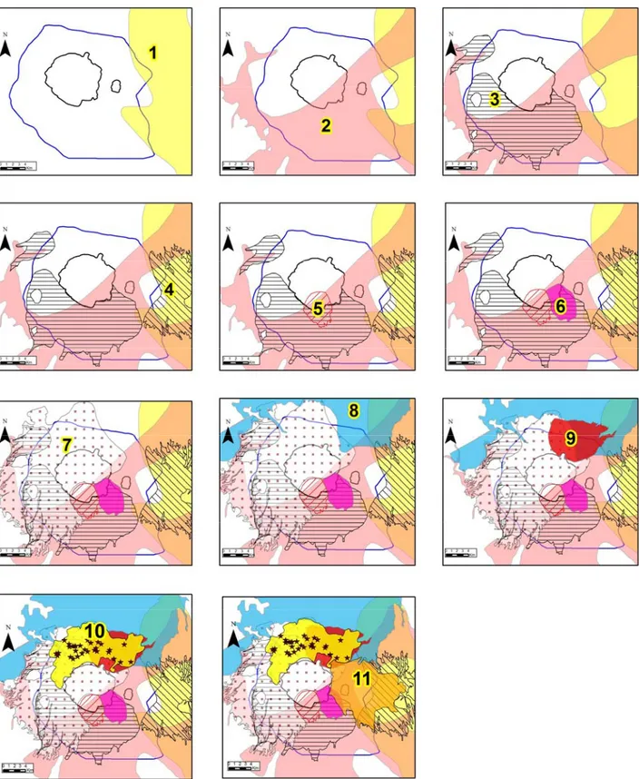
In the sketch of Fig. 2.16 are represented the main steps of the volcanic tectonic evolution of the Sabatini complex.
Figure 2.16: Sketch of Monti Sabatini volcanic complex activity (De Rita, 1993)
I) Pre-volcanic situation as reconstructed through drilling data. The main regional faults are indi-cated. The magmatic acidic activity of Tolfa-Cerite-Manziate area and the hydromagmatic
activ-ity of Morlupo-Castelnuovo di Porto center are indicated.
II) Sacrofano hydromagmatic activity began together with some magmatic activity in the northern sector.
III) Paroxismal stage of the magmatic activity in the Sabatini volcanic complex. Around 0.4-0.3 Myr magmatism with an unsaturated character was active all over the area.
IV) The final phase of Sabatini activity was mainly concentrated in the eastern sector and had hy-dromagmatic character.
1 = products with mainly magmatic character; 2 = products with mainly hydromagmatic character; 3 = prod-ucts with mainly phreato-magmatic character; 4 = neoauthoctonous units (outcropping and covered by vol-canic products); 5 = allochtonous units. They extended below the volvol-canic cover also when a reduced
thick-ness of neoauthoctonous units was present; 6 = Meso-Cenozoic calcareous units, the same symbol indicate areas where these units were actually below volcanics but at shallow depth; 7 = acidic domes; 8 = scoria cones; 9 = emission fracture system; 10 = magmatic craters and caldera; 11 = hydromagmatic edifices; 12 =
hydromagmatic craters and calderas; 13 = phreati-magmatic craters; 14 = main regional fault system; 15 =hypothetical regional faults systems. (De Rita et al., 1993)
2.3HYDROGEOLOGICAL SETTING- DEVELOPMENT OF THE CONCEPTUAL MODEL
A conceptual model of a ground-water flow and hydrologic system is an interpretation or working description of the characteristics and dynamics of the physical hydrogeologic system. The purpose of the conceptual model is to consolidate site and regional hydrogeologic and hydrologic data into a set of assumptions and concepts that can be evaluated quantitatively. Development of the concep-tual model reuquires the collection and anlysis of hydrogeologic and hydrologic data pertinent to the aquifer system under investigation. (ASTM, D5447-04)
Reconstruction of a conceptual model is the first step in approaching groundwater models. In the present study, it was considered the aquifer present in volcanic deposits, as unique main aquifer, on the basis of the geologic and hydrogeologic understanding.
The aim of this study is to better understand the aquifer-Bracciano lake interactions, by developping an useful tool for the management of water resources with a special attention to the lake.
From a geologic point of view it was analyzed the hydraulic behavior of the different volcanic de-posits with the aim to identify areas with a homogenous hydraulic behavior. It was also analyzed the presence of pre-volcanic low permeability sediments below volcanic deposits, which constitute the main surface of hydraulic discontinuity, with a function of base-floor for the conceptual model. The presence of low permeability sediments, located along the perimeter of the area, constitutes the boundary for the model.
Figure 2.17: Geologic sections with a qualitative indication of permeability characteristics of different beds. Sabatini volcanic district is constituted by a big number (hard to quantify) of vents. There are sev-eral strombolian centers of emission (scoria and tuff cones) and there are many fractures from which lavas and explosive volcanic products were erupted (Fig. 2.16 and 2.17). The volcanic activ-ity is characterized by magmatic and hydromagmatic products. Emission centers are present in the east sector of Morlupo, Sacrofano and also in the edges of the volcanic tectonic depression of Brac-ciano. Alternating volcanic activity and interruption periods, the action of atmospheric agents and the variability of the volcanic materials, induced variable stratigraphic conditions not comparable to sedimentary context. Only in vents more marginal areas volcanic products assumed more uniform characteristics, from the view of water circulation, and could be assimilated to continuous sedimen-tary formation.
Hydraulic circulation has particular local conditions influenced by the upper part of the low perme-ability sediments, its thickness variations and lithological characteristics of the underlying forma-tion. The permeability of volcanic deposits is very variable, it depends from volcanic activity prod-ucts: hydromagmatic deposits can be consider to be generally low permeable, on the other side sco-ria cones porosity is predominantly permeable. Another factor conditioning the deposits permeabil-ity is if the cooling process was fast or slow.
The circulation of hydrothermal fluids tends to waterproof a porous and highly permeable deposit, with the deposition of zeolites mineral, as the case of the “tufo rosso a scorie nere” ignimbrite, with low permeability lithoid and zeolites local minerals inserted in a predominant pozzolana highly po-rous and permeable unit.
Figure 2.18: Extension of main volcanic deposits in the study area, following time scale from older to more recent units: 1.TGT (Yellow Tiberina Tuff); 2.TRSNS (Sabatini Red tuff with black scoria); 3.LP-TRSNS (lava post TRSNS); 4.TGS (Sacrofano yellow tuff);5. TVV (Vigna di Valle tuff); 6.TPP (Pizzo Prato tuff); 7.TBR (Bracciano tuff); 8. TRSNV (Vicano Red tuff with black scoria); 9. LP-TRSNV (lava post TRSNV);
10. SC-L(Scoria cones and North Bracciano lava ); 11. HYDRO (Hydromagmatic products of Baccano, Stracciacappa East centers)
Fig 2.18 shows the deposition, step by step, of the main volcanic deposits in the study area. Within each volcanic deposit, the hydraulic properties have peculiar characteristics and may also vary greatly, as previously mentioned, according to deposition processes or subsequent alterations. Vol-canic deposits affect water circulation not only within a single deposit but also at catchment scale by determining the hydraulic conductivity of the various deposits and their connections.
To this extent, after describing the hydraulic properties of volcanic rocks, the analysis of water cir-culation was performed through the observation of the reconstructed water table from 2009 field data in comparison with previously acquired piezometric maps. Starting from the ancient volcanic deposits emplaced in the eastern part (TGT, 1 in Fig. 2.18). The paroxysmal explosive eruption that produced the emplacement of the “tufo rosso a scorie nere” Sabatino (TRSNS, 2 in Fig. 2.18), changes strongly the paleo-morphology of this sector (as well as the eastern). Pyroclastic deposits 10 to 25 m thick were deposited. These deposits of TRSNS, having predominant pozzolana charac-teristic, highly permeable in depressed paleo-morphology, were transformed, with cooling and deposition of zeolites in tuff lithoid reddish, fractured permeability and modest porosity. For its permeability in pozzolana facies, its thickness, even higher than 20 meters, and extension across the area, TRSNS could be considered one of the main aquifer in Sabatini context. The unity of TRSN Sabatino emerges fairly continuous at the edge of the volcanic district. This unit is considered a good stratigraphic indicator: its distribution must have been influenced by topographical conditions existing prior to its emplacement and not present in the high structural of Baccano-Cesano (Cioni, 1993), still morphologically prominent at the time of deposition (De Rita et al., 1993).
After the deposition of TRSNS intense volcanic products, mainly Strombolian lava, a massive (170 km2) lava sequence, with overall thickness locally exceeding 30 meters was emplaced at south of Bracciano Lake (LP_TRSNS, 3 in Fig. 2.18). This layer of lava, with dispersed deposits of pumice-fallout ashes and scoria, is permeable due to fracturing and locally (in bed or on the roof of a single flow) along the scoriaceous facies debris related to the flow of lava.
In the western sector (study area) Bracciano tuff (erupted about 177,000 years BP, 7 in Fig. 2.18). also determines the groundwater circulation for its high porosity, its thickness and its extension. These aquifers are connected, at least locally, through their erosion and tectonic contacts.
In the eastern sector the TRSNS include the aquifer, in addition to fallout and pyroclastic deposits connected to the initial center of Sacrofano.
In the area including Vigna di Valle and the eruptive center of La Conca, two volcanic deposits older than Tufo di Bracciano are present: Tufo di Vigna di Valle ( deposit phase 5 in Fig. 2.18) and the pyroclastic flow deposit of Pizzo Prato (deposit phase 6 in Fig. 2.18). These deposits would be emplaced in rapid succession (De Rita et al., 1993) in a phase of tectonic collapse of river Arrone
valley area between Anguillara and Martignano. Their permeability varies from porous to very po-rous with thickness higher than 10 m in Vigna di Valle and Pizzo Prato chaotic thick deposits with pumice. The southern part of the study area can be considered as a high permeability zone, consid-ering the superimposed volcanic deposits (see later for further discussion).
In this area the presence of high structural pre-volcanic Meso-Cenozoic substrate, has conditioned by its collapse (common to many other volcanic districts) the emplacement of a powerful series of deposits associated with hydromagmatic centers of Baccano, Martignano Stracciacappa, Laguscello, Polline, Trevignano, La Conca, located in the eastern sector of the study area. These layers, mainly ash and of low permeability, previously determined the presence of former lakes, nowadays dried (as Baccano and Stracciacappa), the presence of shallow aquifer and constitute a vertical “barrier” to the main volcanic aquifer located in the more permeable volcanic deposits above desribed (TRSNS, TBR, LP-TRSNS). This situation is represented in Fig 2.17 section 2.
Deposits associated to hydromagmatic centers have mainly low permeability, even if they can be locally very permeable due to sandy scoriaceous layers, strongly influencing the groundwater movement in the eastern and north-east sector.
In the studied volcanic context, the presence of many surfaces of hydraulic discontinuities has to be considered together with possible presence of several local aquifers. To this extent it was performed the reconstruction of the main hydraulic discontinuities constituted by the pre-volcanic low perme-ability sediments, as the roof of one main volcanic aquifer, that well represent the situation at a ba-sin scale.
2.3.1 Reconstruction of hydraulic discontinuity surface
The substrate on which volcanic vents formed was particularly complex and consisting of at least four geologic types, with complex mutual structural relations:
- Allochthonous pelitic-arenaceus, calcareous.marl and clay sediments; - Limestone and limestone marl;
- Sediment cycle autochthonous Neogene, clay and sandy-clay; - Acid volcanic deposits of Tolfa-Cerite-Manziana sector.
Therefore an important step consisted in the “review” of the volcanic basement surface.
These units, so heterogeneous in terms of permeability, are interconnected both vertically (direct contacts via faults or trust, depositional contacts) and horizontally (contacts via direct or reverse faults, intrusive contacts as the case of dominant acid complex of Tolfa and Cerite-Manziana dis-trict), thus increasing the complexity of the prevolcanic substrate.
The bottom of the aquifer is constituted of the low permeability sediments belonging to volcanic substrate.
It was possible to start from the base volcanic surface produced by the project Joint venture ENEL-VDAG-URM (1994). In this previous work the pre-volcanic sediments were not subdivided accord-ing to their hydraulic properties, hence in the present study this aspect was investigated to differen-tiate between low-permeability and permeable pre-volcanic sediments.
A first challenging step was gathering geologic information useful to individuate modifications to the basement surface: geologic maps, sections and stratigraphic logs.
Collected information were a total of 729 stratigraphic logs from different sources:
431 stratigraphic logs retrieved from ISPRA (Istituto Superiore per la Protezione e la Ricerca Am-bientale) database. These data were collected in accordance with the regulation of private well (L. 464/84);
74 stratigraphic logs relative to the Regional Administration database;
103 stratigraphic logs from the Hydrogeology laboratory of Roma Tre University;
111 stratigraphic logs relative to ENEL databases, built in the 70’s as part of ENEL geothermal re-search projects.
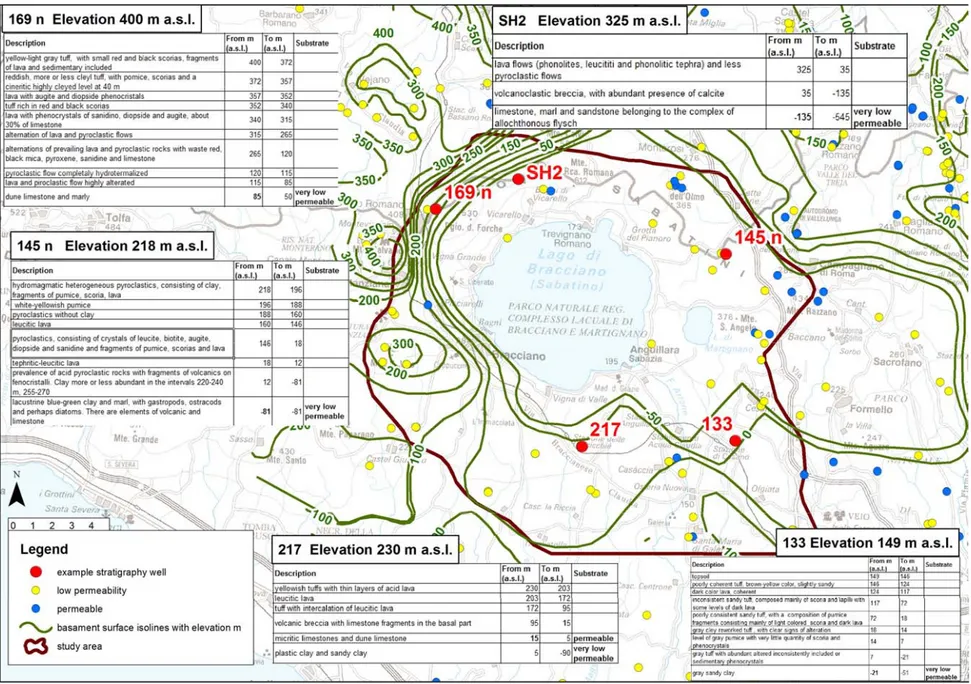
Data quality was very variable and affected by drilling techniques, competence of report author, etc. In Fig. 2.19 are shown all the points with stratigraphic log that have been considered and analyzed. Only 123 points, inside and around the area, could be used to the low permeability surface recon-struction, because they cross all volcanic deposits and reach pre-volcanic sediments, having infor-mation on the hydraulic properties of the pre-volcanic sediments. In Fig 2.19 are also reported five tables relative to the stratigraphic logs of the corresponding red points indicated in the map. These
tables provide an example on what which kind of information was possible to gather. The surface reconstructed from the Enel project was included in a GIS environment as isobaths. The elevations of the low permeability pre-volcanic sediments, taken from stratigraphic logs, were selected. A TIN (Triangulated Irregular Network) was constructed from isobaths (mass points) and point data related to the stratigraphic logs (points) and then converted into a GRID.
Tectonics was also used to reconstruct the abovementioned surface. All the faults affecting the pre-volcanic basement were selected and included in the reconstruction process, as elements of discon-tinuity (polylines barrier). The output GRID and isobaths from GIS elaboration were then checked, and inserted as bottom information in the model, as described in Chapter 4.
The trend of the main hydraulic discontinuity surface, is very articulated. In the western part of the study area the volcanic deposits decrease in thickness and the pre-volcanic sediments outcrops, ex-erting a role of hydraulic barrier to groundwater flow. In the southern part there is an increase of the pre-volcanic sediments (isobaths 100 m a.s.l. in the Santa M. Galeria area), which acting as a barrier to the groundwater flow, divide it into two fluxes (with southeast and southwest direction). In the southern part the outcrops of pre-volcanic sediments appear inside valleys, producing springs aligned with the streams. In the eastern part the thickness of volcanic rocks reaches the higher val-ues of the area (around 500-600 m of volcanic deposits). Fig. 2.20 represents the topography surface and pre-volcanic low permeability top surface, consider as the bottom of the aquifer.
2.3.2 Water table reconstruction and groundwater flow analysis
Once analyzed the hydraulic behavior of the main volcanic deposits and the trend of substrate sur-face, now will be presented the results of a measurement campaign performed in 2009, during this work of study.
The survey campaign was carried out during spring and summer 2009 static water level was meas-ured in 238 wells, 15 springs distributed all over the area and its surroundings. Flow measurement of the principal streams in the study area was also performed (Fig. 2.21 and Fig. 2.22).
Data collected were elaborated and a piezometric surface was man-drown (Fig. 2.21) to better elu-cidate the aquifer-lake and stream-aquifer connections and exchanges. The idea was also to obtain a “photography” of the actual situation to compare with previous representations of the piezometric surface made by Camponeschi & Lombardi, 1968 and by the Hydrogeology laboratory of Roma Tre University, in which this work od study has been elaborated in 2002 (Capelli et al., 2005).
Figure 2.21 – Piezometric map (survey campaign 2009)
In Fig. 2.21 measured wells have been divided in several classes of different depth, considering real depth if data avaiable and considering the “minimum well depth”, calculated from the difference between quota elevation and measured water table, in case of missing data. Another factor that has
been taken into account were conditions measurement was taken (static water table or dynamic wa-ter table).
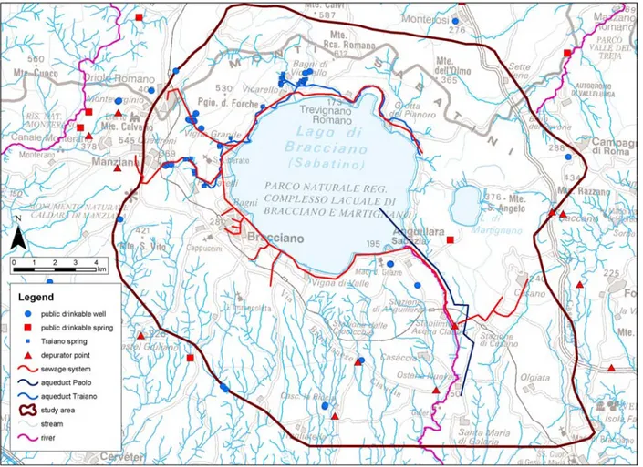
Figure 2.22 – Gauging stations in the area
The quantification of the flow in different sectors is needed to perform water budget calculation, important component to build the groundwater model.
Several stream flow measurements were conducted in Bracciano area, in 1981/1982, in 1999 and in 2002: survey campaigns conducted by the Hydrogeology Laboratory of University of Roma Tre. A survey campaign in 1968 conducted by Lombardi and Giannotti, one in 1992 (Boni et al., unpub-lished 1992), another in 1995 (Aquaital S.R.L., 1997).
All the before mentioned survey campaign did not cover the whole study area, so the comparison could not be generalized to all the sampled streams in 2009. Analyzing discharges with centripetal direction towards the lake, it is possible to observe a flow decrease from the flow measured in 1992 (Boni et al., unpublished 1992). In winter 1992 the discharge was 150 l/s (considering only the northern streams), while in summer 2009 total amount of water drained to the lake was only 30 l/s. In the Table 2.3.b (Annex B) all streams measurement are reported and in the Table 2.3.a, the sea-sonal total amount of water drained to the lake is calculated in different years.
The streams located in the northwest side of the lake (Grotte Renara , Fiora , Vicarello and Val D’Aia) have several springs that feed Traiano aqueduct, active since roman period. The water com-pany ACEA declared that the average water drained by the Traiano aqueduct drainage varies from 50 to 200 l/s. This water has to be considered as outflow of hydrogeological basin.
Table 2.3.a: Total contribution of the streams with a centripetal direction towards the lake
Season Year l/s
winter 1992 151.0
summer 1995 50.7
winter 1995 60.7
summer 2009 32.4
Total lake inflow
In the southeast area Valchetta creek drains water from the hydrogeologic basin of Bracciano (Fig 2.21). In Table 2.4.b (Annex B) measured values, from different survey campaigns, are reported and in Table 2.4.a the seasonal total amount of water drained by the southeast area of the basin, com-puted for different years. The value of 341.7 l/s included both contribution of B28 and B35 stations (code in Fig. 2.22), in the estimation of study area drain water, it has to be consider only the B28 station contribute (115.6 l/s).
Table 2.4.b: Total contribution of the streams draining the southeast side
Season Year l/s winter 1999 294.4 summer 1999 14.0 winter 1981-1982 101.0 summer 1981-1982 500.0 summer 2009 341.7
Total water drained the southeast side
In the southern part of the area streams are located draining from southwest side of the basin. In the Table 2.5.b (Annex B) all values are reported and a Table 2.5.a, the total seasonal amount of drained water by streams is computed for different years.
Table 2.5.a: Total contribution of the streams draining southwest side Season Year l/s winter 1981 109.0 summer 1981 49.0 summer 2002 37.0 summer 2009 87.3
Total water drained
Arrone River, effluent of Bracciano Lake, flows near Fregene (Tyrrenian coast) after running about 37 km, the collection area of surface water (river basin considering also Bracciano Lake) covers an area about 200 km2. In 1700 a dam was built near the beginning of Arrone River. On this artificial spillway some jets have been positioned at a height of 163.4 m a.s.l.. These jets enter into use dur-ing phases of exceptional floods when the lake level exceeds safe altitude. Accorddur-ing to data pro-vided by the water agency ACEA (Lombardi & Giannotti, 1969), in the period 1943-1963, only six years the lake has overflowed naturally, with a complessive flow about 5.106 m3/year. During this period Arrone flow rates were solely linked to the groundwater supply, not being recharged by the lake.
Table 2.6:Arrone river discharge in 1968 (a), in 1981 (b); in 1995 (c) and in 2009 (d) Map
code
Stream Elevation (m a.s.l.)
Year Season FLOW m3/s A1 Arrone river 167.3 1968 summer 0.000 A2 Arrone river 165.0 1968 summer 1.010 A3 Arrone river 158.0 1968 summer 0.906 A5 Arrone river 136.0 1968 summer 0.993
A6 Arrone river 44.0 1968 summer 1.266
b. Map
code
Stream Elevation (m a.s.l.)
Year Season FLOW m3/s A1 Arrone river 167.0 1981 winter 0.010 A1 Arrone river 167.0 1981 summer 0.010 A5 Arrone river 136.0 1981 winter 0.020 A5 Arrone river 136.0 1981 summer 0.010
c. Map
code
Stream Elevation (m a.s.l.)
Year Season FLOW m3/s A3 Arrone river 158.0 1995 summer 0.000 A3 Arrone river 158.0 1995 winter 0.004 A5 Arrone river 136.0 1995 summer 0.075 A5 Arrone river 136.0 1995 winter 0.124
Map code
Stream Elevation (m a.s.l.)
Year Season FLOW m3/s A1 Arrone river 167.0 2009 summer 0.000 A3 Arrone river 158.0 2009 summer 0.000 A4 Arrone river 142.0 2009 summer 0.030 A5 Arrone river 136.0 2009 summer 0.188
These Tables show a quite variable flows with time. In some points, where Lombardi and Giannotti in 1968 measured flow of 1000 l/s, the river bed is now dry.
Comparing the data reported by Lombardi and Giannotti with those acquired during the field cam-paign carried out in summer 1995 and in July 2009, it can be drawn a completely different situation in terms of flow rates. In both campaigns the flow at the Lake effluent of Bracciano Lake (first measurement) is zero because of the artificial barrier that isolated the lake. As reported by Lombardi and Giannotti (1969), it beginning to have a sustained flow in Mola Vecchia (1010 l/s), a few hundred meters downstream from Lake effluent.
A second measurement was made at Valle Trave bridge, where the comparison between the two campaigns apparently explains the changes occurred in the last 30 years. Lombardi and Giannotti measured flow slightly less than the previous section (906 l/s), assuming a section of the river in which the water was drained by the aquifer. In 2009 a dry riverbed was observed in this point. Marked difference was also registered in the flow at Osteria Nuova (Fig. 2.22, code A5): 993 l/s in 1967, and 187 l/s in 2009.
From the data listed above this decrease in flow could be attributed to the change of the piezometric surface elevation, with a general reduction that led the river to be dry for a few sections or sensibly reduce its flow. The lack of recharge may be attributed to a change in the level of Bracciano Lake as suggested by Lombardi and Giannotti (1969). The average level of the lake in April 1967 is 1.32 (± 0.02 m, ACEA data) compared to 0 hydrometric set at 161.74 m (163.06 m ), this data confirms that in that time the lake did not exceed the bulkhead in Anguillara (the overflow is 30 cm higher). Lombardi and Giannotti hypothesized a direct water supply from the lake to the alluvial Arrone de-posits, because, despite they had not project design, considering the age of the construction of the bulkhead, they guessed that the river was not isolated only at the surface but also through at deeper strata. The water of the lake, then infiltrated among the river sediments, re-emerges a little further downstream, approximately near Mola Vecchia, where the terrain elevation is almost the same of the lake level (163 m). At this point the first measure of flow in the river bed with considerable flow was performed. In July 2009, the Bracciano Lake level was 0.66 m on the 0 hydrometric (162.4 m a.s.l.), and below the level preciously recorded. It means that the water flowing through the alluvial deposits can not come out directly in a short distance from the Lake effluent, but probably further
downstream. During 2009 measurements, there were no larger flows than 1967, so probably by lowering the lake level has also changed the way of recharge to Arrone River. Now the river drains the regional aquifer and does not receive a direct recharge from the lake through river sediments. The observed Arrone flux of 0.157 m3/s was measured in a gauge station (A5 in Fig. 2.22) placed some kilometres upstream of the edge of the model domain. It has to be consider the amount of 0.1 m3/s water discharged by the depurator point two kilometres upstream from the A5 measured sta-tion (Fig. 2.28). All things considered, a value of 0.240 m3/s for the whole outflow of the Arrone inside the study area was judged reasonable.
In the study area during summer 2009 total drain outflow measured was around 0.5 m3/s, in addi-tion to a variable volume of 0.05 - 0.2 m3/s. of water drained by Traiano aqueduct from the streams located in the northwest side of Lake Bracciano. Other contribution of 0.1 m3/s has to be considered in the Baccano area, where an artificial drainage system (built to dry the former wetland) collects water discharged downstream (code B25, Fig. 2.22). Galeria stream (measured in location code B23 with absent flow) drains around 0.05 in the last tract. Considering all contributions, a total amount of drain outflow from study area can be estimated to be around 0.75 m3. In Table 2.7 above men-tioned information are listed and each contribution location could be see in Fig. 2.22.
Table 2.7: Total contribution of the streams draining the study area
m3/s
contribution of the streams with a centripetal direction
towards the lake 0.0324
contribution of the streams draining the southeast side 0.1156 contribution of the streams draining southwest side 0.0873
Arrone river drainage 0.24
Galeria stream drainage, last tract 0.05 Baccano area drainage contribution 0.1 northwest drainage contribution, captured by
Traiano aqueduct 0.12
TOTAL 0.7453
Total water drained in the study area (2009)
In last 40 years several piezometric maps have been designed for the Bracciano area, in this work will be considered the piezometric map relative to 1967-1978 survey campaign made by Campone-schi and Lombardi (1968) and the piezometric map relative to 2002 survey campaign carried out by Hydrogeology Laboratory of the University Roma Tre (Capelli et al, 2005). Both maps consider the existence of one main aquifer inside volcanic deposits. In the present study the same approach was kept in the reconstruction of piezometric surface. Analyzing three piezometric surfaces (Fig. 2.21; Fig. 2.23; Fig. 2.24) it is possible to observe the presence of a high gradient area located in the north
west of the lake (in 1968, 2002 and 2009). In piezometric map from 1969, the strong effect of the drains on the piezometric lines in the North West zone is clearly visible, this drainage “disappears” in the following representation of the piezometric surface. It indicates the lowering of the water ta-ble.
In the southern sector piezometric lines trend matches in all three reconstructions, with a visible lowering of water table from 1967-68 to 2002 and 2009.
The hydraulic behavior of the volcanic deposits, hosting the aquifer, could be derived by the recon-structed piezometric maps.
Figure 2.23: Piezometric map (Camponeschi and Lombardi, 1968)
Figure 2.24: Piezometric map 2002 (Capelli et al., 2005)
To improve the understanding of hydraulic behavior of the volcanic deposits, were studied also pumping test results. The available information about hydraulic conductivity in the study area from pumping tests results are only 12 (Fig 2.25), there are some data coming from pumping tests, made by the local potable water company or by owners of the wells. Unfortunately none of these pumping tests have the information about the influence of the withdrawal observed in some nearby piezome-tres. Only few of these pumping tests could be related to a stratigraphic log, so most of the data could not be used.
It is necessary to reflect on which observations are representing the scale that the model study has and the discretization of the numerical groundwater model. A short term pumping tests represent an area near the pumping well, eventually not representing the model grid scale that will be used in this study (100 m). It can be problematic to use measured values of hydraulic conductivity directly in the model, since the hydraulic conductivity has a local “meaning” and is scale dependent (Sonnen-borg & Henriksen, 2005). The following type model has been proposed to describe K’s dependence on scale (Neuman, 1994; Shculze-Makuch et al., 1999)
K = cVm, V≤ Vm [m/s] Eq. 2.2
where V is the volume of geologic material that is included in the measurement; m is a scaling ex-ponent and c is a constant which theoretically describes the hydraulic conductivity of the V=0.
When a heterogeneous aquifer is modelled as a homogeneous entity, there will necessarily be a mis-take, while some sites will be simulated with a too high head level and elsewhere will be simulated with too low head levels. One criterion can be to consider if the mean of the head residuals between observed and simulated head is near zero, it will generally be considered an acceptable approach.
Figure 2.25: Wells hydraulic conductivity information (labels: in pink the well depth and in black the K val-ues)
Considering the hydrogeological basin of Bracciano, to describe water circulation, the area was subdivided in the sub-basins indicated in Fig. 2.25, taking into consideration the following charac-teristics:
• thickness of the aquifer (calculated from the difference between the elevation of the piezo-metric surface related to 2009 campaign survey and the elevation of the pre-volcanic base-ment)
• piezometric trend
• the presence of areas of hydraulic closure, where low permeability deposits outcrops surface flow
• hydraulic characterization of volcanic deposits.
Sub-basin 1. The North-West Sector
At the north-west and west of Lake Bracciano were found prevolcanic sediments in outcrops. These sediments are characterized as clay and flysch and they represent a support above lake level. No groundwater inflow enters the sub-basin 1 from outside, due to the presence of clay and flysch structural border. From here the clay and the flysch dip to east-south direction. The lowering of the contact surface between flysch and volcanic deposits is connected to the presence of volcanic tonic discontinuities with a concentric distribution (Fig. 2.15). These faults are related to the tec-tonic collapse of Lake Bracciano. In the higher relief the thickness of the permeable volcanic depos-its is smaller due to the presence of low permeability prevolcanic sediments at high elevations, go-ing toward the lake the thickness rapidly increases. In this basin the aquifer is limited in the upper part by umpermeable deposits and it is drained by the lava and other high permeability sediments. In Fig. 2.17, in the geologic section number 3, it is represented the above mentioned situation. Het-erogeneous volcanic rocks have here a quite low equivalent hydraulic conductivity (linked to erup-tive fissure fractures or faults presence).
In the piezometric map made by Camponeschi e Lombardi (1968), the piezometric lines appear strongly conditioned from the draining streams Fiora, Vicarello and Val d’Aia. In the following pie-zometric maps (2002 and 2009), the lines have a trend much more regular, the elevation of the wa-ter table is lower and so the wawa-ter table inwa-tercepts streams at lower elevations. Due to the few an-chor points present in this sub-basin, the subjective interpretation affects the reconstruction of the piezometric surface, that strongly indicate a steep trend. The basin 1 (together with the sub-basin 2) gives the higher contribution to lake groundwater inflow.
Sub-basin 2. The Northern Sector
In this area the aquifer thickness has values around 100 and 200 m. The hydraulic connection with the Vicani volcanic aquifer is dynamic and there is no structural closure. It could be hypothesized a groundwater contribution from the Vicani aquifer to this sub-basin and more in general to Brac-ciano hydrogeological basin. From piezometric maps it is possible to observe a dynamic seepage, but it can be that below the water surface a component of the flux direct to the south exists (from north where water table elevation is generally higher, to the south where its elevation is lower). If there was a contribution to groundwater coming from another hydrogeological basin, it should be considered in the global hydrogeological balance. It seems likely an external contribution and the mathematical model could help to evaluate the correctness of this hypothesis.