Dipartimento di Informatica
e Studi Aziendali
Structure of Business Firm Networks and
Scale-Free Models
Maksim Kitsak, Massimo Riccaboni,
Shlomo Havlin, Fabio Pammolli
Structure of Business Firm Networks and
Scale-Free Models
Maksim Kitsak, Massimo Riccaboni, Shlomo Havlin,
Fabio Pammolli and H. Eugene Stanley
Dipartimento di Informatica
e Studi Aziendali
DISA Working Papers
The series of DISA Working Papers is published by the Department of Computer and Management Sciences (Dipartimento di Informatica e Studi Aziendali DISA) of the University of Trento, Italy.
Editor
Ricardo Alberto MARQUES PEREIRA [email protected]
Managing editor
Roberto GABRIELE [email protected]
Associate editors
Flavio BAZZANA [email protected] Finance
Michele BERTONI [email protected] Financial and management accounting
Pier Franco CAMUSSONE [email protected] Management information systems
Luigi COLAZZO [email protected] Computer Science
Michele FEDRIZZI [email protected] Mathematics
Andrea FRANCESCONI [email protected] Public Management
Loris GAIO [email protected] Business Economics
Umberto MARTINI [email protected] Tourism management and marketing
Pier Luigi NOVI INVERARDI [email protected] Statistics
Marco ZAMARIAN [email protected] Organization theory
Technical officer
Paolo FURLANI [email protected]
Guidelines for authors
Papers may be written in English or Italian but authors should provide title, abstract, and keywords in both languages. Manuscripts should be submitted (in pdf format) by the corresponding author to the appropriate Associate Editor, who will ask a member of DISA for a short written review within two weeks. The revised version of the manuscript, together with the author's response to the reviewer, should again be sent to the Associate Editor for his consideration. Finally, the Associate Editor sends all the material (original and final version, review and response, plus his own recommendation) to the Editor, who authorizes the publication and assigns it a serial number.
The Managing Editor and the Technical Officer ensure that all published papers are uploaded in the international RepEc publica-tion database. On the other hand, it is up to the corresponding author to make direct contact with the Departmental Secretary re-garding the offprint order and the research fund which it should refer to.
Ricardo Alberto MARQUES PEREIRA
Dipartimento di Informatica e Studi Aziendali Università degli Studi di Trento
Via Inama 5, TN 38100 Trento ITALIA Tel +39-0461-882147 Fax +39-0461-882124
Structure of Business Firm Networks and Scale-Free Models
Maksim Kitsak,1 Massimo Riccaboni,2 Shlomo
Havlin,1, 3 Fabio Pammolli,1, 4 and H. Eugene Stanley1 1Center for Polymer Studies, Boston University,
Boston, Massachusetts 02215, USA
2Department of Computer and Management Studies , University of Trento, Trento, Italy 3Minerva Center and Department of Physics,
Bar-Ilan University, Ramat Gan, Israel
4IMT Institute for Advanced Studies, Lucca, Italy (Dated: December 24, 2008)
Abstract
We study the structure of business firm networks in the Life Sciences (LS) and the Information and Communication Technology (ICT) sectors. We analyze business firm networks and scale-free models with degree distribution P (q) ∝ (q + c)−λ using the method of k-shell decomposition. We find that the LS network consists of three components: a “nucleus,” which is a small well con-nected subgraph, “tendrils,” which are small subgraphs consisting of small degree nodes concon-nected exclusively to the nucleus, and a “bulk body” which consists of the majority of nodes. At the same time we do not observe the above structure in the ICT network. Our results suggest that the sizes of the nucleus and the tendrils decrease as λ increases and disappear for λ ≥ 3. We compare the k-shell structure of random scale-free model networks with the real world business firm networks. The observed behavior of the k-shell structure in the two industries is consistent with a recently proposed growth model that assumes the coexistence of both preferential and random regimes in the evolution of industry networks.
I. INTRODUCTION
Many real-world complex systems are described as graphs or networks [1–7]. Networks appear in various areas of science such as physics, biology, computer sciences, economics and sociology [3–7]. Real networks, despite their diversity, share many common properties. Some real networks have been found to be “small-world” [3, 8–10]: despite their large size, the typical distance between nodes is very small, of order of log(N) or less [3,11, 12], where N is the number of nodes. Also, some real networks are scale-free (SF) with a power-law tail in their degree distribution
P (q) ∝ (q + c)−λ, (1)
where q is the number of links per node, λ and c are distribution parameters [13–16]. Many statistical physics and mathematical techniques have been successfully applied to study network structure including percolation [12,17–21], scaling [6,7,11], partitioning [22], box covering [23–26], k-core percolation [27, 28] and k-shell decomposition [29] . The latter has been recently used to study the topology of the Internet at the autonomous system (AS) level [30]. It has been found that the AS Internet network can be decomposed into three distinct components:
(i) The nucleus consists of highly connected nodes (hubs) and constitutes a tiny fraction of the network (≈ 0.5%).
(ii) The tendrils (≈ 25%) are the subgraphs that connect to the network exclusively via the nucleus.
(iii) The remaining nodes (≈ 75%) of the network constitute the bulk body. Unlike the tendrils, the nodes in the bulk remain connected even if the nucleus is removed. The appearance of the three components led to the association of the AS Internet structure with that of a jelly-fish model [30]. For an alternative jelly-fish structure see also Ref. [31]. The nucleus plays a crucial role in data transfer throughout the Internet. If the nucleus is damaged or blocked, nodes in the tendrils cease to communicate with other nodes both in the bulk body and in other tendrils. However, the nodes in the bulk body can still communicate with each other, but less efficiently since the average path length between them almost doubles [30]. The network of workplaces in Sweden [32,33] was also shown to
possess a jelly-fish structure. Mean field analysis of the k-shell structure [34, 35] focuses on random networks with a given degree distribution P (q).
In the present work we adopt the same methodology to address the long-standing question of how long does a typical leader in an industry maintain its position. This question has attracted continuing attention in the economics and management literatures over the past generation [36]. Two rival views exist. The first asserts that leadership tends to persist for a ’long’ time while the second one emphasizes the transience of leadership positions due to radical innovation and “leapfrogging competition”. The Life Sciences (LS) sector is generally cited as an archetypal example of stability of industry leaders [37], while on the contrary the Information and Communication Technology (ICT) sector is widely considered as a good example of high market turnover and instability [39]. We study the k-shell structure of the LS and ICT industry in order to test these views and better understand the reasons behind the higher stability of the leading firms in the LS sciences as compared to the ICT sector. The networks of LS and ICT firms are networks of nodes representing firms in the worldwide LS and ICT industries with links representing the collaborative agreements among them [26,37–39]. We also conduct a numerical analysis of model SF networks in order to better understand their k-shell structure. We study how the size and the connectivity of the three components of random SF model networks depend on the SF parameters. We compare the k-shell structure of SF models with that of the LS and ICT industry networks in order to get a better insight into the growth principles of the industry networks.
The rest of the manuscript is organized as follows: in Section II we define the k-shell decomposition and apply it to both real and model SF networks. We then analyze the leadership in the industry networks from the k-shell perspective. In Section III we conduct a systematic analysis of the properties of the three components of model SF networks. In section IV we compare the results for SF models with those observed in the two industrial networks. We conclude our manuscript in Section V with a discussion and summary.
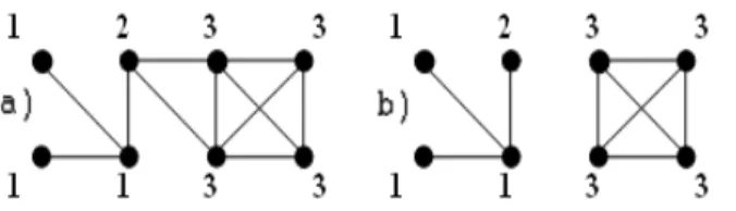
II. K-SHELL, K-CORE, AND K-CRUST
We start the process of the k-shell decomposition [30, 34] on a network by removing all nodes with degree q = 1. After the first iteration of pruning, there may appear new nodes with degrees q = 1. We keep on pruning these nodes until only nodes with degree q ≥ 2 are
left. The removed nodes along with the links connecting them form the k = 1 shell. Next, we iterate the pruning process for nodes of degree q = 2, thereby creating the k = 2 shell. We further continue the k-shell decomposition for higher values of q until all nodes of the network are removed. As a result each node in the network is assigned a k-shell index k. The largest shell index is called kmax, which is also the total number of shells in the network,
provided all shells below kmax exist. The k-crust is defined as the union of all k-shells with
indices smaller than k. Similarly, the k-core is defined as the union of all nodes with indices greater or equal k. (See Fig. 1for demonstration.) As we explain later, the set of nodes in the kmaxshell is called nucleus provided there is a large number of nodes (tendrils) connected
to the network exclusively via the kmax shell.
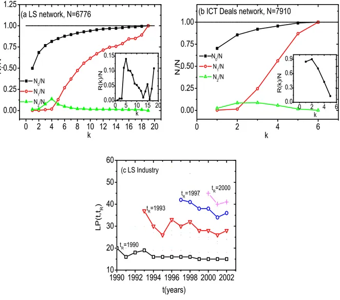
We analyze the k-shell structure of LS and ICT industrial sectors in time periods between 1990 and 2002 and between 1990 and 2000 respectively. Data have been collected from several sources including: Repec, Windhover, Bioscan, Pharmadeals, company press releases and news. The LS network expanded linearly since the mid-1970s while the ICT network took off in the 1990s and grew exponentially for a decade [see Fig. 2(a) and the inset]. The total number of firms in the LS is N = 6, 776 and in the ICT is N = 7, 759. These sizes refer to the largest connected component of each of the networks at the last year of observation. Both industrial networks feature SF degree distributions with λ ≈ 2.5, c ≈ 4. (LS) and λ ≈ 3.4, c ≈ 6. (ICT) which we estimate with the maximum likelihood method [see Fig. 2(b)]. We use the Kolmogorov-Smirnov test in order to examine the goodness of fit of the degree distributions. The obtained p-values for 1000 trials are 0.24 and 0.33 for the LS and the ICT industry networks respectively.
We next apply the k-shell decomposition procedure to the LS and the ICT networks. For each k-crust we calculate N0, the total number of nodes in the k-crust, N1, the size of the
largest connected component in the k-crust and N2, the size of the second largest component
of the k-crust. As seen in Fig. 3, the LS network consists of kmax= 19 shells while the ICT
network (which consists of comparable number of firms) has only kmax = 6 shells. The size
of the largest cluster in the k-crust starts growing rapidly after k = 4 and k = 2 in the LS and the ICT networks respectively. At these values of k, the size of the second largest cluster in the k-crust reaches a maximum. The above behavior of the k-crust components is consistent with the existence of a second order phase transition in the k-crust structure [30]. The type of the phase transition taking place at the k-shell decomposition is similar
to that of targeted percolation in SF networks [21,40].
Unlike in the ICT network, the size of the largest connected component N1 in LS network
undergoes a large jump N1(k = 19) − N1(k = 18) = 745, while the total size N0 of the
crust experiences only a small change N0(k = 19) − N0(k = 18) = 43 (See Fig. 3(a)).
This can be explained as follows [30]. Approximately 10% of the he LS network are firms (which we call “tendrils”) that prefer to sign collaborative agreements exclusively with the 43 firms that form the shell k = kmax = 19 (which we call the nucleus). Typically, each
of these firms (tendrils) signs a small number of agreements with firms in the nucleus and, therefore, has small degree. Thus, the tendrils are removed in the decomposition of the first few shells. However, being connected exclusively to the nucleus in the kmax = 19
shell, the tendrils do not contribute to the largest connected component of the k-crust until the last kmax shell is decomposed. It is the inclusion of the tendrils firms into N1(k)
at the decomposition of the kmax shell that results in the observed jump in N1(k). The
appearance of the three components—the nucleus, the tendrils and the bulk body—allows one to associate the structure of the network of LS firms with that of the jelly-fish similar to the Internet at the Autonomous System level [30]. Interestingly, we do not observe the a similar jump in N1(k) in the ICT network (See Fig. 3(b)).
In both LS and ICT industry sectors the kmaxshells include market leaders such as Pfizer,
GSK, Novartis, J&J, Sanofi-Aventis, Bayer in the LS network and Microsoft, IBM, AT&T, Yahoo, Cisco, AOL, Time Warner and Google in the ICT network. We find that the LS network tendrils are mostly composed of the new start up firms and their university partners. On the one hand, start up firms preferentially attach to market leaders. On the other hand, market leaders compete to sign exclusive deals with new and promising start up firms. We also notice the remarkable stability of the LS nucleus: once a particular firm enters the nucleus it is very likely to remain there for many years.(See Fig. 3c) On the contrary, in the ICT sector there is more emphasis on how to integrate different technologies and markets [39]. Thus, there are more deals between firms of the same size and age but in different technological and market areas. As a consequence, the k-shell of the ICT network is more unstable and heterogeneous which may explain why we do not detect the emergence of a nucleus such as in the LS sector.
As discussed above, one can in general calculate the size of the nucleus Sn as the total
Sn= N0(kmax) − N0(kmax−1). (2)
The increase in N1(k) at k = kmax is comprised by the inclusion of tendrils St and the
nucleus Sn. Thus, the size of tendrils can be calculated as
St= N1(kmax) − N1(kmax−1) − Sn. (3)
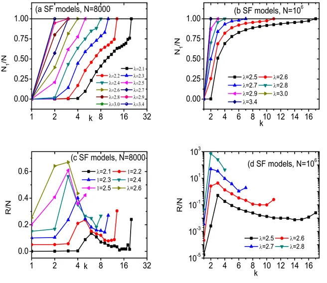
As seen in Fig. 2(b), both the LS and the ICT industrial networks exhibit a SF degree distribution. Hence, in order to better understand the substructures of real networks— the nucleus, the tendrils, and the bulk components—we analyze the k-shell structure of the random SF models which were generated using the configurational approach [41]. We calculate the k-shell structure of random SF networks with c ≥ 0, and degree distribution exponent λ ∈ [2, 3]. For our simulations (Fig. 4) we choose networks sizes of N = 8, 000 (which is comparable to the size of the LS and ICT industry networks) and N = 106 in
order to test the influence of finite size effects.
Fig. 4 shows that both the number of shells kmax and the jump in the largest connected
component N1(k) decrease as the exponent λ increases. As the jump becomes less
pro-nounced it becomes harder to detect it motivating us to introduce a quantitative criterion for the emergence of the three distinct components. We define the rate of change of the largest connected component size as
R(k) ≡ N1(k) − N1(k − 1). (4)
We compare the increase of the largest connected component R(k) at k = kmax with that
at k = kmax−1. The jump in N1(k) results in
R(kmax) > R(kmax−1). (5)
We use Eq. (5) as a criterion for the existence of a nucleus and tendrils.
By examining R(k) plot we observe in the case of N = 8, 000 (Fig. 4c), that SF models with λ > 2.5 already do not have a nucleus and tendrils. However, for N = 106 we do
observe nucleus and tendrils in SF models for λ ≤ 2.7. (Fig. 4d). These observations suggest that all SF networks with 2 < λ < 3 have a nucleus and tendrils provided N is sufficiently large. The above observations for SF models agree with the fact that we observe jelly-fish topology for LS network (λ = 2.5) and do not observe it for ICT network λ = 3.4.
However, SF model networks with N = 8000 with λ = 2.5 and λ = 3.4 have kmax = 5
and kmax = 2 respectively, while the measured kmax in LS and ICT networks (which have
the same λ values) are kmax = 19 and kmax = 6. The observed difference in kmax between
industry networks and SF models with similar parameters suggests to further explore the k-shell structure of SF networks and consider SF model networks with c > 0 values in P (q) (as found in the LS and the ICT networks).
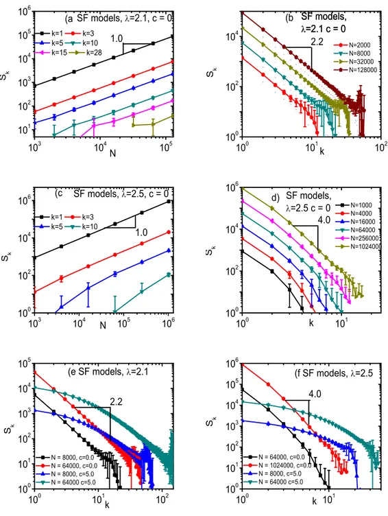
III. K-SHELL PROPERTIES OF SCALE-FREE NETWORKS
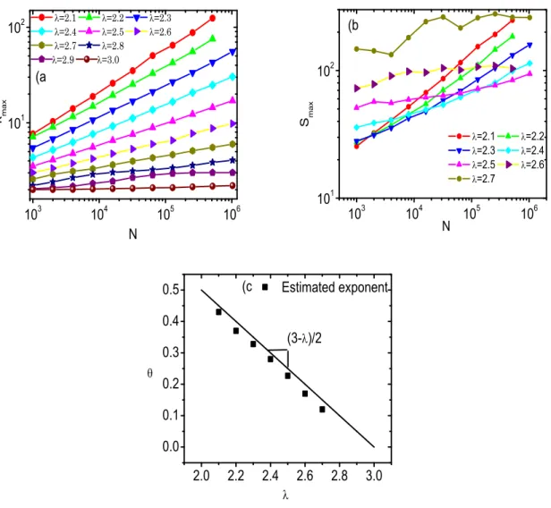
SF networks may or may not have a jelly-fish structure, depending on the degree distri-bution P (q) and size N. In order to better understand the k-shell structure of SF networks, we calculate the sizes of the k-shells as a function of N and λ. For each pair of values N and λ we generate 103−104 realizations of SF models and calculate the average number of
shells kmax constituting the network as well as their average size Sk (see Fig.5). For small
k values, Sk is proportional to N. As the size of the network increases new shells start to
appear. When the size increases further, the new shell growth stabilizes and becomes also proportional to N (See Fig.5a,c). This result indicates that the size of each shell constitutes a certain finite fraction of the network and this fraction decreases with increasing k. The analytical analysis of k-core structure [34] leads to
Sk ∝k−δ, (6)
where
δ = 2
3 − λ. (7)
Hence δ ≈ 2.2 for λ = 2.1 and δ ≈ 4.0 for λ = 2.5, which agrees with our simulations. [Figs. 5(b) and 5(d)]. The appearance of c > 0 in the SF degree distribution significantly increases kmax [see Figs.5(e) and 5(f)]. However, the asymptotic dependence of k-shell sizes
seems to remain the same as k approaches kmax: Sk∼k−δ [Figs.5(e) and 5(f)].
One can estimate the total number of shells in a random SF network of size N as follows. Since every shell constitutes a fixed fraction of N it follows that Sk ∝Nk−δ. The last shell
kmax needs to possess at least one node Smax ≡Sk=kmax ∼1, which leads to
Indeed, the total number of shells kmax seems to increase as a power law with the network
size N [Fig. 6(a)]. The smaller is λ the faster is the growth of kmax. As seen from Fig. 6(c), the estimated exponents 1/δ agree with those predicted by Eq. (8). Note that Eq. (8) together with
δ = 2/(3 − λ) (9)
is consistent with the fact that networks with λ > 3 do not have a k-shell structure.
The dependence of Smax on N can be regarded as a crossover from the small N regime
with N < Nc(λ), where there is no nucleus, to the power-law regime for N > Nc(λ) where
Smax ∼ Nτ (λ) ( Fig. 6b). We relate the observed crossover with the emergence of the
nucleus and tendrils in SF networks for N > Nc(λ). The critical size of SF networks, Nc(λ),
corresponding to the emergence of the nucleus and tendrils in SF networks seems to increase as λ increases. In the N < Nc regime the size of the last shell Smax increases with λ, which
can be explained by the fact that SF networks with higher λ have fewer shells. On the other hand, in the power-law regime, the size of the last shell, Smax, (which now becomes
the nucleus Sn) is smaller for larger values of λ.
IV. EVOLUTION AND STRUCTURE OF THE LS AND ICT INDUSTRY
NET-WORKS
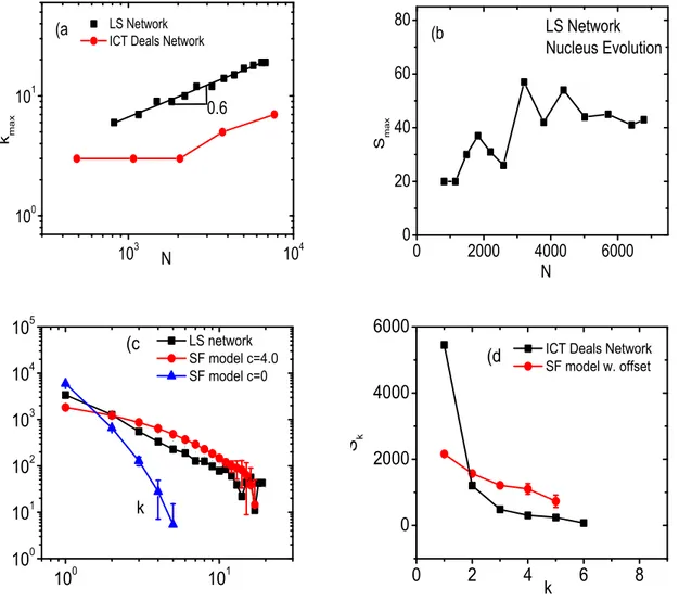
We further analyze the k-shell structure of the LS and ICT industry networks. The number of shells kmax in the LS industry grows as a power-law function of its size,
kmax∼Nθ, (10)
and reaches kmax = 19 in 2002. Our estimates yield θ ≈ 0.6 (Fig. 7a). We find that the
number of shells in ICT sector, kmax, also grows and reaches kmax = 6 in 2000. Note that
Snfor the LS network exhibits fluctuations for N ∈ [2000, 5000] and stabilizes for N > 5000
(See Fig. 7b). As seen in Fig. 7(c,d), the sizes of shells Sk decrease as a function of their
index k in both networks. As we notice in Section II, the observed shell sizes Skas well as the
number of shells kmax, measured for the LS and ICT networks, deviate from those obtained
from SF models with c = 0. We expect for random SF models with c = 0, λ = 2.5 and λ = 3.4 and similar sizes as LS and ICT to find kmax = 5 and kmax = 2 respectively. Also,
from the observed shell sizes The measured Kolmogorov-Smirnov statistic is D ≈ 0.137 . [see Fig. 7(c)]. The observed differences can be explained by taking into account the offset c in SF degree distribution of both networks. The adjustment of the degree distribution of random SF models with c = 4.0 and c = 6.0 allows one to obtain similar patterns Sk
which are in fair agreement with the industry networks, as seen in Figs. 7(c) and7(d) (The Kolmogorov-Smirnov statistic in this case, D ≈ 0.074).
As seen above, the offset c > 0 in the SF degree distribution plays a crucial role in the formation of the k-shell structure of industry networks. A possible reason for the emergence of c > 0 in growing networks is the combination of preferential attachment with random attachment in network evolution [42]. The coexistence of preferential attachment regime with random collaborative agreements was suggested to take place in industry networks [37]. The random component is caused by the fact that sometimes firms choose exclusive relationships and novelty, and do not prefer to make deals with hub firms. Even though the coexistence of both preferential and random regimes seems to be crucial in the formation of the industry networks, it does not fully reproduce the k-shell structure of LS and ICT industries. We believe that a better understanding of the evolution of the LS and ICT networks may be achieved by further improvements of the modeling.
V. DISCUSSION AND SUMMARY
We use the k-shell decomposition to analyze the structure of the LS and ICT industry networks. We find that the firms in the LS industry can be naturally divided into three components: the nucleus, the tendrils and the bulk body. The nucleus of the LS industry consists mostly of the market leader firms while the tendrils are typically comprised of small start-up firms that preferentially make deals with leading firms which are in the nucleus. We show that the nucleus of the LS industry exhibits remarkable stability in time. In contrast, the ICT industry does not have a nucleus. We also analyzed the dependence of the k-shell structure of SF model networks on N, λ and c. We observed the formation of the nucleus and the tendrils in SF networks only for λ < 3. The number of shells kmaxand the size of the
nucleus Sn are larger for SF networks with c > 0 compared to those with c = 0. Our results
can partly explain the k-shell structure of LS and ICT industry networks. The coexistence of preferential and random attachment leads to the appearance of the offset c > 0 in the
SF degree distribution P (q) ∼ (q + c)−λ [42]. Thus, the appearance of c > 0 in the degree
distribution of LS and ICT networks might be explained by the interplay of random and preferential agreements among firms in the industries [37].
Acknowledgments
We thank ONR, European project DAPHNET,the Israel Complexity Center, Merck Foun-dation (EPRIS project) and Israel Science FounFoun-dation for financial support. We thank L. Braunstein, S. Carmi and L. K. Gallos for valuable discussions.
[1] P. Erd¨os and A. R´enyi, Publ. Math. Inst. Hung. Acad. Sci. 6, 290 (1959). I
[2] P. Erd¨os and A. R´enyi, Publ. Math. Inst. Hung. Acad. Sci. 5, 17 (1960). [3] B. Bollobas, Random Graphs (Cambridge University Press, 2001). I
[4] S. Wasserman and K. Faust, Social Network Analysis, (Cambridge University Press, 1999). [5] S. N. Dorogovtsev and J. F. F. Mendes, Evolution of Networks (Oxford University Press,
2003).
[6] M. Newman, A. L. Barab´asi and D. J. Watts, The Structure and Dynamics of Networks (Princeton University Press, 2006). I
[7] S. Bornholdt and H. G Schuster Handbook of Graphs and Networks (WILEY-VCH, New York, 2001). I,I
[8] S. Milgram, Psychol. Today 2, 60 (1967). I
[9] D. J. Watts and S. H. Strogatz, Nature 393, 440 (1998).
[10] R. Albert, H. Jeong, and A.-L. Barab´asi, Nature 401, 130 (1999). I
[11] R. Cohen and S. Havlin, Phys. Rev. Lett. 90, 058701 (2003). I,I
[12] R. Cohen and S. Havlin Complex Networks: Structure, Stability and Function(Cambridge University Press, Cambridge, in press 2008). I,I
[13] H.A. Simon, Biometrika 42, 425 (1955). I
[14] D. de S. Price, J. Amer. Soc. Inform. Sci. 27, 292, (1976). [15] A.-L. Barab´asi and R. Albert, Science 286, 509 (1999).
[17] S. Kirkpatrick, Rev. Mod. Phys. 45, 574 (1973). I
[18] D. Stauffer and A. Aharony, Introduction to Percolation Theory, 2nd Edition (Taylor and Francis, New York, 2004).
[19] A. Bunde and S. Havlin, Fractals and Disordered Systems, 2nd Edition (Springer, Berlin, 1996).
[20] R. Cohen, K. Erez, D. B. Avraham, and S. Havlin, Phys. Rev. Lett. 85, 4626 (2000).
[21] D. S. Callaway, M. E. J. Newman, S. H. Strogatz and D. J. Watts, Phys. Rev. Lett. 85, 5468 (2000). I,II
[22] G. Paul, R. Cohen, S. Sreenivasan, S. Havlin and H. E. Stanley, Phys. Rev. Lett. 99, 115701 (2007); Y. Chen, E. Lopez, S. Havlin, and H. E. Stanley, Phys. Rev. Lett. 96, 068702 (2006).
I
[23] C. Song, S. Havlin, and H. Makse, Nature 433, 392 (2005). I
[24] C. Song, S. Havlin, and H. Makse, Nature Physics 2, 275 (2006).
[25] K. I. Goh, G. Salvi, B. Kahng, and D. Kim, Phys. Rev. Lett. 96, 018701 (2006).
[26] M. Kitsak, S. Havlin, G. Paul, M. Riccaboni, F. Pammolli, and H. E. Stanley, Phys. Rev. E. 75, 056115 (2007). I
[27] B. Bollobas, Graph Theory and Combinatorics: Proceedings of the Cambridge Combinatorial Conference in honor of P. Erd¨os, 35 (Academic, New York, 1984) I
[28] S. B. Seidman, Social Networks, 5, 269 (1983). I
[29] J. I. Alvarez-Hamelin, L. Dall’Asta, A. Barrat and A Vespignani, Networks and Heterogeneous Media 3, 371 (2008). I
[30] S. Carmi, S. Havlin, S. Kirkpatrick, Y. Shavitt, and E. Shir, Proc. Natl. Acad. Sci. USA 104, 11150 (2007). I,II,3
[31] L. Tauro, C. Palmer, G. Siganos, and M. Faloutsos, Global Internet (Nov. 2001). I
[32] WWW.SCB.SE I
[33] Y. Chen, G. Paul, R. Cohen, S. Havlin, S. P. Borgatti, F. Liljeros and H. E. Stanley, Phys. Rev. E 75, 046107 (2007). I
[34] S. N. Dorogovtsev, A. V. Goltsev, and J. F. F. Mendes, Phys. Rev. Lett. 96, 040601 (2006).
I,II,III
[35] A. V. Goltsev, S. N. Dorogovtsev, and J. F. F. Mendes, Phys. Rev. E 73, 056101 (2006). I
[37] L. Orsenigo, F. Pammolli, and M. Riccaboni, Res. Policy 30, 485 (2001). I,IV,V
[38] F. Pammolli and M. Riccaboni, Small Business Economics 19(3), 205 (2002). [39] M. Riccaboni and F. Pammolli, Research Policy 31, 1405 (2002). I,II
[40] R. Cohen, K. Erez, D. ben-Avraham, and S. Havlin, Phys. Rev. Lett., 86, 3682 (2001). II
[41] M. Molloy and B. Reed, Random Struct. Algorithms 6, 161 (1995). II
FIG. 1: Illustration of the k-shell decomposition method. (a) Original network. Nodes are marked by corresponding k-shell indices. Note that the k-shell index does not coincide with the node degree. (b) The 3-crust (left) and the 3-core (right) of the original network.
1992 1996 2000 0.0 2.0k 4.0k 6.0k 8.0k 1992 1996 2000 10 1 10 2 10 3 10 4 N Year LS Industry ICT Industry (a 10 1 10 2 10 3 10 0 10 1 10 2 10 3 10 4 10 1 10 2 10 3 10 0 10 2 10 4 2.4 N ( q > q 0 ) q 0 +c
ICT Deals network
LS Network (b 1.5 N ( q > q 0 ) q 0
FIG. 2: (a) The growth of the largest connected component of LS and ICT industries. The LS industry expands almost linearly while the ICT industry exhibits exponential growth (see inset, a semi-log plot of the ICT network size as a function of time). (b) Cumulative degree distribution N(q > q0) of LS and ICT networks. The inset displays cumulative
0 5 10 15 20 0.00 0.05 0.10 0.15 R ( k) / N k 0 2 4 6 8 10 12 14 16 18 20 0.00 0.25 0.50 0.75 1.00 1.25 N 0 /N N 1 /N N 2 /N (a LS network, N=6776 N i / N k 0 2 4 6 0.00 0.25 0.50 0.75 1.00 N 0 /N N 1 /N N 2 /N
(b ICT Deals network, N=7910
N i / N k 0 2 4 6 0.0 0.3 0.6 0.9 R ( k) / N k 19901992 1994 19961998 2000 2002 10 20 30 40 50 60 t R =2000 t R =1997 t R =1993 (c LS Industry LP ( t , t R ) t(years) t R =1990
FIG. 3: (a) The k-shell structure of the LS network and (b) of the ICT network. Plots of the size of the k-crust, N0; the size of the largest connected component of the k-crust, N1;
and the size of the second largest connected component of the k-crust, N2, as a function of
the k-crust index k. The sizes are normalized with the total number of nodes in the network, N. N2 is multiplied by 100. The transition of the k-crust at shell k = 18 of the
LS network reveals a jelly-fish topology [30]. Since the change in F1 ≡N1/N at the
k = kmax is smaller in the ICT network than in the previous shell k = kmax−1, the ICT
does not have a jelly-fish structure. The insets of (a,b) show the rate R of the largest connected component change as a function of shell index k. (c) The leadership persistence
LP (t, tR) as a function of years in the LS industry. We define LP (t, tR) as a number of
firms that were in the nucleus both at time tR and t. Note that most of the LS firms
1 2 4 8 16 32 0.00 0.25 0.50 0.75 1.00 N 1 / N (a SF models, N=8000 k 2 4 6 8 10 12 14 16 0.00 0.25 0.50 0.75 1.00 k N 1 / N (b SF models, N=10 6 =2.5 =2.6 =2.7 =2.8 =2.9 =3.0 =3.4 1 2 4 8 16 32 0.0 0.2 0.4 0.6 (c SF models, N=8000 R / N k =2.1 =2.2 =2.3 =2.4 =2.5 =2.6 2 4 6 8 10 12 14 16 10 -5 10 -3 10 -1 10 1 10 3 k R / N (d SF models, N=10 6 =2.5 =2.6 =2.7 =2.8
FIG. 4: (a,b) The k-shell structure of random SF models with (a) N = 8000 and (b) N = 106 nodes are shown for comparison. Note that λ = 3.4 curve overlaps with that of
λ = 3.0. (c,d) The rate of the largest connected component change, R, as a function of shell index k for (c) N = 8000 and (d) N = 106. Note that in order to avoid the overlap of
curves in (c,d) we subsequently shift the plots with respect to each other by the additive factor 0.05 in (c) and the multiplicative factor of 10 in (d). The sizes of the nucleus and
the tendrils decrease as λ increases. The nucleus and the tendrils disappear in (a,c) for N = 8000 at λ > 2.5 and in (b,d) for N = 106 at λ > 2.7.
10 3 10 4 10 5 10 1 10 2 10 3 10 4 10 5 10 6 N S k 1.0 (aSF models, =2.1, c = 0 k=1 k=3 k=5 k=10 k=15 k=28 10 0 10 1 10 2 10 0 10 2 10 4 SF models, =2.1 c = 0 2.2 S k N=2000 N=8000 N=32000 N=128000 (b SF models, =2.1 c = 0 k 10 3 10 4 10 5 10 6 10 0 10 2 10 4 10 6 S k N 1.0 (c SF models, =2.5, c = 0 k=1 k=3 k=5 k=10 10 0 10 1 10 0 10 2 10 4 10 6 4.0 N=1000 N=4000 N=16000 N=64000 N=256000 N=1024000 SF models, =2.5 c = 0 k S k d) 10 0 10 1 10 2 10 0 10 1 10 2 10 3 10 4 10 5 N = 8000, c=0.0 N = 64000, c=0.0 N = 8000, c=5.0 N = 64000 c=5.0 2.2 (e SF models, =2.1 S k k 10 0 10 1 10 0 10 1 10 2 10 3 10 4 10 5 10 6 4.0 N = 64000, c=0.0 N = 1024000, c=0.0 N = 8000, c=5.0 N = 64000 c=5.0 (f SF models, =2.5 S k k
FIG. 5: Sizes of k-shells, Sk, for SF random models with c = 0 (a,b) λ = 2.1 and (c,d)
λ = 2.5 as a function of (a,c) N and the k-shell index (b,d) k. Note that sizes of k-shells increases proportionally to N. (e,f) Sizes of k-shells, Sk, for SF networks with c = 5.0 and
(e) λ = 2.1, (f) λ = 2.5. SF models with c = 5.0 have significantly larger number of shells, kmax, compared to SF models with the same λ and c = 0. Sk in SF models with c = 5.0
decreases significantly slower as a function of k compared to SF models with the same λ and c = 0 in the small k region. In the large k region both types of SF models with c = 0.0
10 3 10 4 10 5 10 6 10 1 10 2 k m a x N =2.1 =2.2 =2.3 =2.4 =2.5 =2.6 =2.7 =2.8 =2.9 =3.0 (a 10 3 10 4 10 5 10 6 10 1 10 2 (b S m a x N =2.1 =2.2 =2.3 =2.4 =2.5 =2.6 =2.7 2.0 2.2 2.4 2.6 2.8 3.0 0.0 0.1 0.2 0.3 0.4 0.5 (c (3- )/2 Estimated exponent
FIG. 6: (a) The total number of shells, kmax, in SF models as a function of N. Note that
kmax∝Nθ. (b) The size of the last shell Smax in the SF model as a function of N. Each
curve crosses over into a power law regime for N ≥ Nc(λ), where Nc(λ) increases with λ.
(c) The calculated exponent θ as a function of λ (symbols). Our calculated values of δ agree with the mean field theory result δ ≈ 2/(3 − λ) (solid line).
10 3 10 4 10 0 10 1 (a 0.6 N k m a x LS Network
ICT Deals Network
0 2000 4000 6000 0 20 40 60 80 S m a x N LS Network Nucleus Evolution (b 10 0 10 1 10 0 10 1 10 2 10 3 10 4 10 5 k (c LS network SF model c=4.0 SF model c=0 0 2 4 6 8 0 2000 4000 6000 (d S k
ICT Deals Network
SF model w. offset
k
FIG. 7: (a) The largest shell index kmax of the LS and the ICT networks as a function of N
calculated for different years. The number of shells kmax of the LS network increases
approximately as a power-law function of the network size kmax ∼Nθ, where θ ≃ 0.6. (b)
Size of the nucleus of the LS network, Sn, as a function of N. Sn exhibits fluctuations as
LS network grows. Unlike in the analyzed SF models, Smax becomes stable for N > 5000.
(c) Sk as a function of the k-shell index k for the LS network (squares). Shell sizes Sk as a
function of k decrease significantly slower than Sk∼k−4, which is expected for a random
SF model with the same λ and c = 0 (triangles). However, the offset introduction of c = 4.0 in the SF degree distribution, P (q), mimics the k-shell structure of the LS network
(circles). (d) Sk as a function of k-shell index k for the ICT network (squares). SF model
with λ = 3.4 and c = 0 does not possess a k-shell structure. However, the introduction of c = 6.0 in the SF degree distribution yields similar k-shell structure (circles), but we