DEPARTMENT OF INFORMATION AND COMMUNICATION TECHNOLOGY
38050 Povo — Trento (Italy), Via Sommarive 14 http://dit.unitn.it/
REACTIVE LOCAL SEARCH FOR MAXIMUM CLIQUE: A
NEW IMPLEMENTATION
Roberto Battiti and Franco Mascia
May 2007
Reactive local search for maximum clique: A new
implementation
Roberto Battiti and Franco Mascia
Dept. of Computer Science and TelecommunicationsUniversity of Trento, Via Sommarive, 14 - 38050 Povo (Trento) - Italy
e-mail of the corresponding author: [email protected]
May 2007
Abstract
This paper presents algorithmic and implementation enhancements of Reactive Local Search algorithm for the Maximum Clique problem [3]. In addition, we build an empirical complexity model for the CPU time required for a single iteration, and we show that with a careful imple-mentation of the data-structures one can achieve a speedup of at least an order of magnitude difference for large size graphs.
1
Introduction
The motivation of this work is to assess how different implementations of the supporting data structures of RLS for the Maximum Clique Problem affect the CPU times.
Let us briefly summarize the context and define our terminology.
Let G = (V, E) be an undirected graph, V = {1, 2, . . . , n} its vertex set, E ⊆ V × V its edge set, and G(S) = (S, E ∩ S × S) the subgraph induced by S, where S is a subset of V . A graph G = (V, E) is complete if all its vertices are pairwise adjacent, i.e., ∀i, j ∈ V, (i, j) ∈ E. A clique K is a subset of V such that G(K) is complete. The Maximum Clique problem asks for a clique of maximum cardinality.
A Reactive Local Search (RLS) algorithm for the solution of the Maximum-Clique problem is proposed in [1, 3]. RLS is based on local search complemented by a feedback (history-sensitive) scheme to determine the amount of diversifi-cation. The reaction acts on the single parameter that decides the temporary prohibition of selected moves in the neighborhood. The performance obtained in computational tests appears to be significantly better with respect to all algo-rithms tested at the the second DIMACS implementation challenge (1992/93)1. The new experimental results motivated also two qualitative changes of the algorithm: the fact that the entire search history is kept for the whole run duration (instead the memory was cleared at each restart in the previous version) and the fact that a new upper bound has been placed on the prohibition value T .
1http://dimacs.rutgers.edu/Challenges/
The following sections present the main algorithmic changes, some optimiza-tions of the C++ code, and finally we develop an empirical complexity model of the CPU time for a single iteration.
2
Algorithmic changes
We refer to [3] for details about the algorithm and for bibliography about dif-ferent approaches for solving the maximum clique problem.
Briefly, the RLS algorithm alternates between expansion and plateau phases, selecting the nodes among the non-prohibited ones which have the highest degree in PossibleAdd. The prohibition time is adjusted reactively depending on the search history. In the “history” a fingerprint of each configuration is saved in a hash-table. Restarts are executed only when the algorithm cannot improve the current configuration within a specified number of iterations.
Reactive-Local-Search 1 2 3 4 5 6 7 8 9 10 11 12 13 14 B Initialization. t ← 0 ; T ← 1 ; tT← 0 ; tR← 0 ;
CurrentClique ← ∅ ; BestClique← ∅ ; MaxSize← 0 ; tb← 0
repeat 2 6 6 6 6 6 6 6 6 6 6 6 4 T ← Memory-Reaction(CurrentClique, T ) CurrentClique ← Best-Neighbor (CurrentClique) t ← (t + 1)
if f (CurrentClique) > MaxSize then 2 4 BestClique ← CurrentClique MaxSize ← |CurrentClique| tb← t if (t − max{tb, tR}) > A then tR← t ; Restart
until MaxSize is acceptable or maximum no. of iterations reached
Figure 1: RLS algorithm, from [3].
Best-Neighbor (CurrentClique) 1 2 3 4 5 6 7 8 9 10 11 12 13 14 15 16 17 18 19 20
Bv is the moved vertex, type is AddMove, DropMove or NotFound type ← NotFound if |S| > 0 then 2 6 6 6 6 6 4
Btry to add an allowed vertex first
AllowedFound ← ({ allowed v ∈ PossibleAdd} 6= ∅) if AllowedFound then
2 4
type ← AddMove
MaxDeg ← maxallowed j∈PossibleAdd{degG(PossibleAdd)(j)}
v ← random allowed w ∈ PossibleAdd with degG(PossibleAdd)(w) = MaxDeg
if type = NotFound then 2 6 6 6 6 6 6 6 4
Badding an allowed vertex was impossible: drop type ← DropMove
if ({ allowed v ∈ CurrentClique} 6= ∅) then »
MaxDeltaPA ← maxallowed j∈CurrentClique DeltaPA[j]
v ← random allowed w ∈ CurrentClique with DeltaPA[w] = MaxDeltaPA else
v ← random w ∈ CurrentClique Incremental-Update(v, type)
if type = AddMove then return CurrentClique ∪ {v} else return CurrentClique \ {v}
Figure 2: Best-Neighbor routine, from [3].
The research presented in this paper considers two kinds of changes to the original RLS version. The first changes are algorithmic and influence the search
Memory-Reaction (CurrentClique, T) 1 2 3 4 5 6 7 8 9 10 11 12 13 14 15 16
Bsearch for clique CurrentClique in the memory, get a reference Z Z ← Hash-Search(CurrentClique) if Z 6= Null then 2 6 6 6 6 6 4
Bfind the cycle length, update last visit time: R ← t − Z.LastVisit Z.LastVisit ← t if R < 2 (n − 1) then » t T ← t return max(Increase(T ), M AX T ) else »
Bif the clique is not found, install it: Hash-Insert(CurrentClique, t) if (t − tT) > B then » tT ← t return Decrease(T ) return T
Figure 3: Memory-Reaction routine, from [3].
Restart 1 2 3 4 5 6 7 8 9 10 11 12 13 14 15 16 T ← 1 ; tT← t
B search for the “seed” vertex v
SomeAbsent ← true iff ∃v ∈ V with LastMoved[v] = −∞ if SomeAbsent then»
L ← {w ∈ V : LastMoved[w] = −∞}
v ← random vertex with maximum degG(V )(v) in L
else v ← random vertex ∈ V PossibleAdd ← V OneMissing ← ∅ forall v ∈ V » MissingList[v] ← ∅ ; Missing[v] ← 0 DeltaPA[v] ← 0 CurrentClique ← {v} Incremental-Update(v, AddMove)
Figure 4: Restart routine.
trajectory, while the second ones refer only to the more efficient implementation of the supporting data structures, with no effect on the dynamics.
The algorithmic changes are the following ones. In the previous version the search history was cleared at each restart, now, in order to allow for a more efficient diversification, the entire search history is kept in memory.
Having a longer memory caused the parameter T to explode on some specific instances characterized by many repeated configuration during the search. Now, if the prohibition becomes much larger than the current clique size, after a maximal clique is encountered and one node has to be extracted from the clique, all other nodes will be forced to leave the clique before the first node is allowed to enter again. This may cause spurious oscillations in the clique membership which may prevent discovering the globally optimal clique.
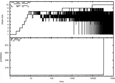
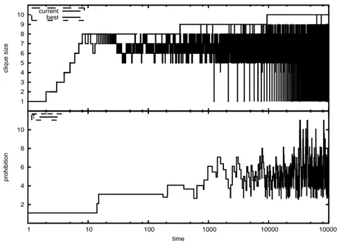
An effective way to avoid the above problem is to put an upper-bound M AX T equal to a proportion of the current estimate of the maximum clique. More specifically, the upper-bound M AX T is set to |BestClique|, being, the size of the best configuration found during the search. Fig. 6 shows the ex-plosion of the parameter T which decreases the average clique size, and Fig. 7 shows how the issue is addressed by putting an upper bound to the prohibition parameter.
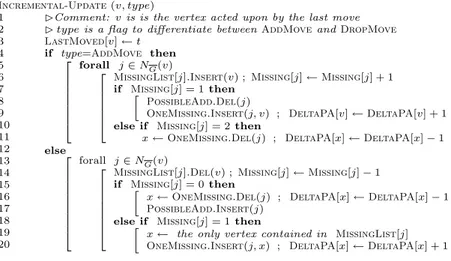
Incremental-Update (v, type) 1 2 3 4 5 6 7 8 9 10 11 12 13 14 15 16 17 18 19 20
BComment: v is is the vertex acted upon by the last move B type is a flag to differentiate between AddMove and DropMove LastMoved[v] ← t if type=AddMove then 2 6 6 6 6 6 6 6 4 forall j ∈ NG(v) 2 6 6 6 6 6 4
MissingList[j].Insert(v) ; Missing[j] ← Missing[j] + 1 if Missing[j] = 1 then
»
PossibleAdd.Del(j)
OneMissing.Insert(j, v) ; DeltaPA[v] ← DeltaPA[v] + 1 else if Missing[j] = 2 then
x ← OneMissing.Del(j) ; DeltaPA[x] ← DeltaPA[x] − 1 else 2 6 6 6 6 6 6 6 6 6 4 forall j ∈ NG(v) 2 6 6 6 6 6 6 6 4
MissingList[j].Del(v) ; Missing[j] ← Missing[j] − 1 if Missing[j] = 0 then
»
x ← OneMissing.Del(j) ; DeltaPA[x] ← DeltaPA[x] − 1 PossibleAdd.Insert(j)
else if Missing[j] = 1 then »
x ← the only vertex contained in MissingList[j] OneMissing.Insert(j, x) ; DeltaPA[x] ← DeltaPA[x] + 1
Figure 5: Incremental-Update routine.
3
Implementation details
The total computational cost for solving a problem is of course the product of the number of iterations times the cost of each iteration. More complex algorithms like RLS risk that the higher cost per iteration is not compensated by a sufficient reduction in the total number of iterations. This section is dedicated to exploring this issue.
The original implementation [3] focused on the algorithm and the appro-priate data structures but did not optimize low-level implementation details. For example, every time a new configuration had to be inserted in the table, the memory needed to store the element was allocated dynamically. The new implementation moved from these on-demand allocations to the more efficient allocation of a single bigger chunk of memory; the memory is used as a pool of available locations to be assigned to the elements when needed. In this way, if one million different configurations are expected, instead of doing one million times expensive system calls, one single call is done at the beginning, and new elements are later added by means of fast pointer assignments.
Moreover, the hash table resolves key collisions by means of chaining. In order to keep the frequent access operation as close to a direct access as possi-ble, these chains have to be kept as short as possible. This has been achieved doubling the size of the hash table when the number of elements inside the table exceeds a specified load factor. More in detail, the hash table is created at the beginning with a default size, along with the corresponding pool of available locations for the expected configuration which are a fraction of the size of the table:
table = new elem*[hash size];
pre alloc = new elem[(int)ceil(hash size * fill factor)];
The initialfill factoris set to 0.6. When there are no more allocations avail-able in the pool, and an element has to be added, the size of the hash tavail-able is doubled. If there is not enough memory for doubling the hash table and
218 436 654 872 1 10 100 1000 10000 100000 prohibition time T 1 2 3 4 5 6 7 8 9 10 clique size current best
Figure 6: Evolution of the size of the current clique during the search, and prohibition parameter T explosion at approximately 33000 iterations, impacting on the clique size. The run is on a gilbert 1100 0.3 instance [2]; x axis is in log scale.
consequently growing the allocation pool, the size of the hash table is kept con-stant and the fill factor increased by 0.2. In the latter case, the access to the elements in the table is less efficient because one resorts more frequently to chaining to resolve possible collisions.
4
Empirical model for cost per iteration
Let us now consider a simple model to capture the time spent by the RLS algo-rithm on each iteration. Most the cost is spent on updating the data structures after each addition or deletion. After a node deletion the complexity for up-dating the data structures is O(degG(v)), degG(v) being the degree of the just moved node v in the complementary graph G. After a node addition the com-plexity is O(degG(v) · |PossibleAdd|), see [3] for more details. Now, because the algorithm alternates between expansions and plateau moves, for most of the run |PossibleAdd| oscillates between 0 and 1. We can therefore make the strong assumption that |PossibleAdd| is substituted with a small constant. In both cases the dominant factor is therefore O(degG(v)). Moreover, since the algorithm selects the nodes having the highest degree among all the candidates, the cost of O(degG(v)) is kept as small as possible.
The computational complexity for using the history data-structure can be
2 4 6 8 10 1 10 100 1000 10000 100000 prohibition time T 1 2 3 4 5 6 7 8 9 10 clique size current best
Figure 7: Evolution of the size of the current clique during the search, with an upper bound on prohibition parameter T . The run is on a gilbert 1100 0.3 instance [2]; x axis is in log scale.
amortized to a O(1) complexity per iteration. The restart operation cannot be amortized: its complexity is O(n) but it is not performed regularly. On the contrary, the number of restarts highly depends on the search dynamics and on the hardness of the instance.
Under the above assumption we decided to propose an empirical model for the time per iteration which is linear in the number of node and the degree:
T (n, degG) = α n + β degG+ γ (1)
The last simplification is given by substituting the average node degree in-stead of the actual degree.
Let us note that the above model is not precise if the size of the Possi-bleAdd set remains large for a sizable fraction of the iterations. For example this is the case when a large graph is extremely dense, and the clique is very large. In this case the size of the PossibleAdd set is a non-negligible factor which multiplies degG(v), impacting significantly the overall algorithm perfor-mance. This happens for the MANN instances in the DIMACS benchmark set which are not considered when fitting the above model.
The fitted model for our specific testing machine is the following:
The fit residual standard errors for α, β and γ are 0.0004, 0.0009 and 0.2765 respectively.
Let us note that the cost for using the history data-structure, which is ap-proximately included in the constant term in the above expression, becomes rapidly negligible as soon as the graph dimension and density of the complemen-tary graph are not very small. In fact the memory access costs approximately less than 50 nanoseconds per iteration while the total cost reaches rapidly tens of microseconds in the above instances.
5
Experimental Results
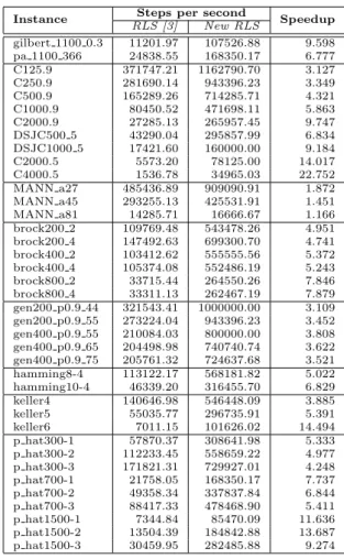
The speedup results reported in Table 1 show the improvement in the steps per seconds achieved by the new version, considering both algorithmic and imple-mentation improvements, for two random graphs [2] and some representative DIMACS instances. Let us note that the obtained speedup is substantial. For example the improvement for large random graphs increases with the graph dimension reaching a factor of 22 for graphs with thousand nodes (C4000.5).
The results of the current investigation show that a careful implementation of the data-structures considering also operating system services like memory allocation achieves a significant reduction of the CPU time per iteration. Be-cause in certain cases one obtains an order of magnitude difference, this aspect is very crucial when comparing two algorithms.
Moreover, the empirical complexity model shows how the cost for keeping the history of the search trajectory is negligible for non trivial graph instances.
References
[1] R. Battiti and M. Protasi. Reactive local search for the maximum clique problem. Technical Report TR95052, ICSI, 1947 Center St. Suite 600 -Berkeley, California, Sep 1995.
[2] Roberto Battiti and Franco Mascia. Reactive and dynamic local search for max-clique, does the complexity pay off? Technical Report DIT-06-027, Department of Information and Communication Technology, University of Trento, April 2006.
[3] Roberto Battiti and Marco Protasi. Reactive Local Search for the Maximum Clique Problem. Algorithmica, 29(4):610–637, 2001.
Instance Steps per second Speedup RLS [3] New RLS gilbert 1100 0.3 11201.97 107526.88 9.598 pa 1100 366 24838.55 168350.17 6.777 C125.9 371747.21 1162790.70 3.127 C250.9 281690.14 943396.23 3.349 C500.9 165289.26 714285.71 4.321 C1000.9 80450.52 471698.11 5.863 C2000.9 27285.13 265957.45 9.747 DSJC500 5 43290.04 295857.99 6.834 DSJC1000 5 17421.60 160000.00 9.184 C2000.5 5573.20 78125.00 14.017 C4000.5 1536.78 34965.03 22.752 MANN a27 485436.89 909090.91 1.872 MANN a45 293255.13 425531.91 1.451 MANN a81 14285.71 16666.67 1.166 brock200 2 109769.48 543478.26 4.951 brock200 4 147492.63 699300.70 4.741 brock400 2 103412.62 555555.56 5.372 brock400 4 105374.08 552486.19 5.243 brock800 2 33715.44 264550.26 7.846 brock800 4 33311.13 262467.19 7.879 gen200 p0.9 44 321543.41 1000000.00 3.109 gen200 p0.9 55 273224.04 943396.23 3.452 gen400 p0.9 55 210084.03 800000.00 3.808 gen400 p0.9 65 204498.98 740740.74 3.622 gen400 p0.9 75 205761.32 724637.68 3.521 hamming8-4 113122.17 568181.82 5.022 hamming10-4 46339.20 316455.70 6.829 keller4 140646.98 546448.09 3.885 keller5 55035.77 296735.91 5.391 keller6 7011.15 101626.02 14.494 p hat300-1 57870.37 308641.98 5.333 p hat300-2 112233.45 558659.22 4.977 p hat300-3 171821.31 729927.01 4.248 p hat700-1 21758.05 168350.17 7.737 p hat700-2 49358.34 337837.84 6.844 p hat700-3 88417.33 478468.90 5.411 p hat1500-1 7344.84 85470.09 11.636 p hat1500-2 13504.39 184842.88 13.687 p hat1500-3 30459.95 282485.88 9.274
Table 1: Speed improvement on random graphs and selected DIMACS bench-mark instances of the new RLS implementation.
![Figure 3: Memory-Reaction routine, from [3].](https://thumb-eu.123doks.com/thumbv2/123dokorg/2947850.23162/5.892.151.563.188.404/figure-memory-reaction-routine-from.webp)