RECORD VALUES FROM A FAMILY OF J-SHAPED DISTRIBUTIONS Ahmad A. Zghoul
1. INTRODUCTION
A class of distributions called a family of J-shaped distributions was introduced by (Topp and Leone, 1955). The distribution function form of a J-shaped distri-bution with scale parameter and shape parameter is
0 ; <0 ( ) 2 ;0 1 ; x x x F x x x
and hence the density has the form
1 2 ( ) 1 x x 2 x ;0 , f x x with 0 and 0 .
The appropriateness of the distribution for modeling life data was emphasized by (Nadarajah and Kotz, 2003). They highlighted the fact that its hazard rate fun-ction is bathtub shaped. Further they derived general formulas for the moments and the central moments of the distribution and provided the maximum likeli-hood estimator of the shape parameter when the scale is known. The dis-tribution of ordered statistics along with their moments and product moments were studied by (Zghoul, 2010).
The bathtub or U-shaped hazard rate functions have many applications in life time modeling. For example, in human populations the death rate is high due to birth defects or infant diseases at infant age, and then it remains constant up to the age of thirties where it increases again. This pattern is common in manufac-tured items. Most parametric models having U-shaped hazard rate function usu-ally involve three or more parameters which in turns raise substantial problems in
statistical inference unless large samples are available. An advantage of the J-shaped family of distributions, which has a U-J-shaped hazard rate function, is that it has only two parameters; namely the scale parameter and the shape parame-ter .
We assume through this work, without loss of generality, that=1, in which case the distribution and the density functions are, respectively, reduced to
0 ; 0 ( ) ( (2 )) ;0 1;0 1 1 ; 1 x F x x x x x (1) and 1 ( ) 2 (1 )( (2 )) ;0 1;0 1 f x x x x x . (2)
In section 2 of this paper we study the distribution of record values from this J-shaped family of distributions. Then, in section 3, moments, product mo-ments, and recurrence relations are obtained. Also, bounds based on Jensens’ inequality for the mean of record values are provided. In section 4, the maximum likelihood estimator for the shape parameter
θ
based on lower record values is derived and its properties are studied. A real life application is investigated in tion 5. Finally, the conclusions and suggestions for further studies is given in sec-tion 6.2. DISTRIBUTION OF RECORD VALUES
Let X X1, 2,...be a sequence of independent and identically distributed random variables. Let (0) 0, (1) 1L L and L n( ) min{ : j Xj XL n( 1)};n2,3,..., then Rn XL n( ),n is the sequence of upper record values. If the inequality 1 sign is reversed then Rn XL n( ) is the sequence of lower record values.
The theory of record values, record times, and inter-record times were first in-troduced by (Chandler, 1952). Since then many research papers have been pub-lished in the subject. Detailed review of records and related bibliography can be found in (Nevzorov, 1987), (Nagaraja, 1988), (Ahsanullah, 1995), (Balakrishnan and Nagaraja, 1998), (Nevzorov and Balakrishnan, 1998), (Arnold et al., 1998), to mention some.
Let R R1, 2,... be a sequence of upper record values from the distribution (1),
[ log(1 ( ))] ( ) ( ) ! n n R F r f r f r n ( )( ( )) 1[ log(1 ( ( )) )] ;0 1 ! n u r u r u r r n ,
where ( )u r r(2 and hence ( ) 2(1r) u r . r)
The joint probability distribution function (pdf) of the set of upper records
1, 2,..., n R R R is 1 1 ,..., 1 1 ( ) ( ,..., ) ( ) 1 ( ) n n i R R n n i i f r f r r f r F r
1 1 1 1 ( )( ( )) ( )( ( )) 1 ( ( )) n n i i n n i i u r u r u r u r u r
.3. MOMENTS AND PRODUCT MOMENTS OF RECORD VALUES
In this section the moments and product moments of record values are de-rived. Recurrence relations for the moments are given. Moreover, we derive a lo-wer bound and an upper bound for the mean of upper records.
Theorem 1: For k=1,2,…, and n=1,2,…, the kth moment of the nth lower record
value is given by:
( )k ( , )(1 )(n 1) n j d k j i
, where d k( ,0) 2 , d( ,1) 2 k k k 2k, and 2 ( 2 1)! 2 ( , ) ! ( )! k jk k j d k j j k j , for j = 2,3,…. (3) Proof: 1 ( ) 1 0 [ log( ( ))] ( ) ( )( ( )) ! n k k k n E Rn r u r u r u r dr n
.Put ( )s u r , then r u 1( ) 1s 1 , hence s 1 ( ) 1 1 0 [ log( )] (1 1 ) ! n k n k n s s s ds n
. (4)A power series expansion for (1 1x)k given by (Gradstein and Ryzhik, 1980), page 21, is: 2 3 4 ( 3) ( 4)( 5) (1 1 ) 2 1 1! 4 2! 4 3! 4 ( 5)( 6)( 7) ... , 4! 4 k k k x k k x k k k x x k k k k x for any real number k and x . 1
Which, alternatively can be written as:
0 (1 1 )k ( , ) j j x c k j x
, where 1 2 2 1 2 ( ,0) 2 , ( ,1) 2 , and ( , ) ( ), for j 2 ! j k j k k i k c k c k k c k j k j i j
. Since (1 1x) (1k 1x)k xk, we have (1 1x)k xk(1 1x)k 0 ( , )( ) k j j x c k j x
0 ( , ) k j j d k j x
, (5)where d k( ,0) 2 , d( ,1) 2 k k k 2k, and for j 2 1 2 1 2 ( , ) ( ) ! j k j i k d k j k j i j
2 ( 2 1)! 2 ! ( )! k jk k j j k j 2 2 ( , ) ( ) k jk B k j j j k j .1 1 ( ) 1 0 0 [ log( )] ( , ) ! n n k j j s d k j s ds n
.Set log( )u s to get:
( )k n 11 ( ) 0 0 ( , ) ! n n k j u j u d k j e du n
1 0 ( , ) n j d k j k j
. In particular, 1 0 [ ] (1, ) 1 ' n n j E R d j j
1 1 1 1 1 1 ... 2 1 4 2 8 3 n n n .Let R R1 , 2,...be a sequence of lower records from the distribution in (1), and
let 1( ), ( ),...k 2 k be the corresponding sequence of the kth moments of 1, 2,...
R R , then we prove the following recurrence relation.
Theorem 2: For k=1,2,…, and n=1,2,…, the kth moments of the nth upper record
value is given by:
( )k ( , )( 1)i k j / (1 )(n 1) n i j i d j k i
.where ( , )d j k are as defined in (5).
Proof: 1 ( ) 1 0 [ log(1 ( ))] ( ) ( )( ( )) ! n k k k n n u r E R r u r u r dr n
.Put ( )s u r , then r u 1( ) 1s 1 , and s 1 ( ) 1 0 [ log(1 )] (1 1 ) ! n k k n s s s ds n
.Expanding as in (5) and following steps similar to those in the proof of Theo-rem 1, the theoTheo-rem is proved.
Theorem 3: For n=1,2,… and k=0,1,2,… ( 1) ( ) ( 1) ( ) 1 1 2( 1)( ) 2 2 ( 1) ( 2 1) ( 2 1) ( 2 1) k k k k n n n n k k k k k k k k . Proof: We have 1 ( ) ( 1) 0 1 2 (2 )( log( ( )) ( ) ! k k k n n n x x F x f x dx n
. (6)From (1) and (2) it is readily seen that x (2–x) f(x) = 2θ (1–x) F(x), so (6) be-comes ( ) ( 1) 2 k k n n 1 1 0 2 (1 )( log( ( )) ( ) ! k n x x F x F x dx n
. (7)Integrating by parts treating xk1(1x) for integration and the rest of the
in-tegrand for differentiation, the r.h.s. of (7) turns out to be
1 1 1 0 1 1 2 ( ) ( log( ( )) ( ) ( log( ( )) ( ) , 1 ( 1)! ! k k n n x x F x f x F x f x dx k k n n
hence ( ) ( 1) ( ) ( 1) ( ) ( 1) 1 1 2 2 2 1 1 k k k k k k n n n n n n k k k k .Arranging terms in the above equation, the theorem is proved.
The following theorem gives upper and lower bounds for the mean of Rn. Theorem 4: For n =1, 2, …, and 0 1, we have ln n un, where
( 1) 1/
1 1 (1 2 n )
n
l and un 1 (2/3)n1.
Proof: As ( ) [ (2g x x x)] is concave, by Jensen’s inequality we have ( ( n)) ( ( n))
g E R E g R ,
which implies that
( 1)
[ (2 )] [ ( )] 1 2 n
n n E F Rn
.
Writing [ (2n n)] as [1 (1 n) ]2 and manipulating, the lower bound is
To derive the upper bound, we have 1 0 ( ) n n rfR r dr
1 0 [ log(1 ( ))] ( ) ! n F r rf r dr n
.Use the transformation u log(1F r( )) to get
1/ 0 [1 1 (1 ) ] ! n u u n u e e du n
.For 0 , we have 1 (1eu)1/ 1 eu, which implies that
/2 1 0 (1 ) 1 (2/3) ! n u u n n u e e du n
.Upon computing lower bounds for the first few records we found that they get tighter as either n or increases.
To derive the product moments of record values we first derive their joint dis-tribution. The joint pdf of the mth and nth record values is given by:
1 2 , 1 1 ( ) log 1 ( ) [ log(1 ( ))] ( , ) 4 ! ( 1)! ( ) ( ) ( ) ,0 1. 1 ( ) m n n m n m m R R m n m n m m n m u r u r u r f r r m n m u r u r u r r r u r
Based on the expansion in (5) the joint moments of R R are given in the fol-m n
lowing theorem.
Theorem 5: For k=1,2,…, l=1,2,…, and for m=1,2,…and n=1,2,…, the joint
mo-ments of R R are m n 3 4 1 2 1 2 3 4 ( ),( ) 2 / 1/ ( ) ( 1) , 3 3 4 3 4 ( 1)i i (1 ) (1 ) k l l i k i n m m m n i i i i i i i i c c i i i
,where c are as defined in (5). i
4. ESTIMATION BASED ON LOWER RECORD VALUES
The joint pdf of the set of lower records R R1 , 2,...,Rn is
1 1 ,..., 1 1 ( ) ( ,..., ) ( ) ( ) n n i R R n n i i f r f r r f r F r
1 1 1 ( ) ( )( ( )) ( ) n n i n n i i u r u r u r u r
.Thus the log likelihood function is given by:
1
log ( ,..., ; )L r rn nlog ( 1)log ( )u rn .
From which the maximum likelihood estimator (MLE) of is found to be
1 ˆ (log ( ))
n
n u R
. (8)
To show that ˆ is an unbiased and consistent estimator for , we have
1 1 1 0 ˆ [ log( ( )) ] ( ) ( log ( )) ( )( ( )) ! n n u r E n u r u r u r dr n
1 0 ! n y y n e dy n
,where the substitution y log ( )u rn is used.
If similar integration is carried out, one obtains
2 ˆ ( ) E = 2 2 ( 1) n n n , and hence 2 ˆ ( ) ; 2 ( 1) Var n n ,
which implies that ˆ (log ( )) 1 n
n u r
is a consistent estimator for .
The density of Yn u R( n)Rn(2Rn) is:
1 1 1 [ log( )] ( log( )) ( ) ! ! n n n n Y y y f y y y n n . (9)
It is clear from (9) that (u R is sufficient and complete statistic for n) . Therefore 1 ˆ (log ( )) n n u r is UMVUE for . (10) 5. AN APPLICATION
Lawless (1982) page 256 fitted a set of data, representing the numbers of cycles to failure for a group of 60 electrical appliances, to a mixture of two Weibull dis-tributions. We reproduce the data (ordered failure times) here:
14 34 59 61 69 80 123 142 165 210 381 464 479 556 574 839 917 969 991 1064 1088 1091 1174 1270 1275 1355 1397 1477 1578 1649 1702 1893 1932 2001 2161 2292 2326 2337 2628 2785 2811 2886 2993 3122 3248 3715 3790 3857 3912 4100 4106 4116 4315 4510 4584 5267 5299 5583 6065 9701
The last observation is about 4 standard deviations larger than the mean so it may be considered as an outlier. We will ignore this data point in our analysis and the data is rescaled by dividing each observation by 7000. The maximum likeli-hood estimator (based on the whole sample) of is computed to be 0.77.
0.2 0.4 0.6 0.8 Data 0.2 0.4 0.6 0.8 1.0 1.2 1.4 Quantile Exponential Distribution P P 0.2 0.4 0.6 0.8 Data 0.2 0.4 0.6 0.8 1.0 1.2 Quantile Weibull Distribution P P (a) (b) 0.2 0.4 0.6 0.8 Data 0.2 0.4 0.6 0.8 Quantile J shaped Distribution P P (c)
Figure 1(a)-(c) – Probability plots for failure data assuming exponential, Weibull, and J-shaped
distri-butions.
Exponential Distribution P-P Weibull Distribution P-P
The probability plots assuming that the data is exponential, Weibull, and J-shaped distribution, respectively are displayed in Figure 1 (a)-(c). These plots are nothing but the inverse of the empirical distribution function under each of the above assumed distributions. Clearly, the J-shaped distribution under study has the best fit compared to the exponential and the Weibull distributions.
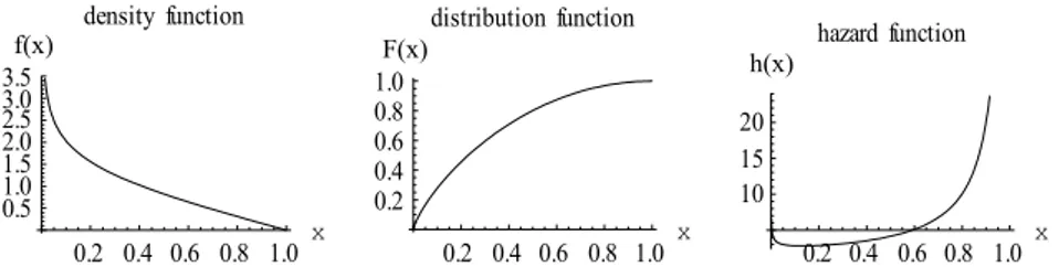
The density, distribution, and the survival functions of the fitted J-shaped dis-tribution are displayed in Figure 2. We notice that the hazard function is almost bathtub-shapes. 0.2 0.4 0.6 0.8 1.0x 0.5 1.0 1.5 2.0 2.5 3.0 3.5f x density function 0.2 0.4 0.6 0.8 1.0 x 0.2 0.4 0.6 0.8 1.0 F x distribution function 0.2 0.4 0.6 0.8 1.0 x 10 15 20 h x hazard function
Figure 2 – The density, distribution, and survival functions of the fitted J-shaped distribution for the
failure data.
Having fitted a J-shaped distribution with =0.77 to the data given above, all theoretical results can be applied to this model. In particular we may obtain the value of the MLE for based on a sequence of lower records obtained upon randomizing the above data. For example, one randomization produces the se-quence 1702, 1091, 165, 142, 34, 14. Based on this sese-quence, applying (10), the MLE for is approximately 0.72. We note that this estimator is somewhat close to the MLE based on the whole sample obtained to be 0.77.
6. CONCLUSIONS AND FURTHER STUDIES
We have studied in this article the distributional properties of record values from a J-shaped family of distributions. Based on lower records, we derived re-currence relations and bounds for moments and product moments of record val-ues. Moreover, the maximum likelihood estimator of the shape parameter was obtained and shown to be consistent, sufficient, complete and UMVUE estima-tor. Further a real life data has been fitted to this family of distributions.
In addition to further investigation of the pertinence of these distributions in survival and reliability analysis, one may study the prediction of future record values from this family of distributions. Also, studies to obtain the MLE estimator of the scale parameter, based on both complete and record samples, can be conducted.
Department of Mathematics AHMAD A. ZGHOUL
College of Sciences The University of Jordan
REFERENCES
M. AHSANULLAH, (1995), Introduction to Record Statistics, NOVA Science Publishers Inc., Hungtington, New York.
B.C. ARNOLD, N. BALAKRISHNAN, H.N. NAGARAJA, (1998), Records, John Wiley and Sons. K.N. CHANDLER, (1952), The distribution and frequency of record values, “Journal of the Royal
Sta-tistical Society”, Series B, 14, pp. 220-228.
I.S. GRADSHTEYN, I. M. RYZHIK, (1980), Table of Integrals, Series, and Products, Academic Press, Orlando, Florida, USA.
J.F. LAWLESS, (1982), Statistical models and methods for lifetime data, John Wiley and Sons. S. NADARAJAH. S. KOTZ, (2003), Moments of Some J-Shaped Distributions, “Journal of Applied
Statistics”, 30(3), pp. 311-317.
H.N. NAGARAJA, (1988), Record Values and Related Statistics- A review, “Communications in Sta-tistics- Theory and Methods ”, 17, pp. 2223-2238.
V.B. NEVZOROV, (1987), Records, “Theory of Probability and Applications”, 32(2), pp. 201-228.
V.B. NEVZOROV, N. BALAKRISHNAN, (1998). A Record of Records, “In Handbook of Statistics- 16: Order Statistics: Theory and Methods”, pp. 515-570, North-Holland, Amsterdam, The Netherlands.
C.W. TOPP, F.C. LEONE, (1955), A family of J-Shaped Frequency Functions, “Jounal of the Ameri-can Statistical Association”, 50, pp. 209-219.
A.A. ZGHOUL, (2010), Order statistics from a family of J-shaped distributions, to appear in “MET-RON”, LXVIII, n. 2, pp. 127-136.
SUMMARY
Record values from a family of J-shaped distributions
A family of J-shaped distributions has applications in life testing modeling. In this pa-per we study record values from this family of distributions. Based on lower records, re-currence relations and bounds as well as expressions for moments and product moments of record values are obtained, the maximum likelihood estimator of the shape parameter is derived and shown to be consistent, sufficient, complete and UMVU estimator. In ad-dition, an application in reliability is given.