From regional to local climate scenario: toward an integrated strategy for climate impacts reduction

(1)

Doctoral school in Science

Civil and Environmental Protection – XIV cycle

FROM REGIONAL TO LOCAL CLIMATE

SCENARIO:

TOWARD AN INTEGRATED STRATEGY FOR

CLIMATE IMPACTS REDUCTION

PhD candidate:

Lorenzo Sangelantoni

Tutor:

(2)

(3)

Abstract

Lying at the center of Mediterranean basin, identified as one of the most sensitive area to anthropogenic climate change, Italy is expected to be particularly susceptible to global climate change. Italian peninsula represents an interesting example of challenging climate-change scenario definition case of study. Given the significant latitudinal extension, its climate results heterogeneous, covering a transitional zone where both semi-arid and temperate climate dynamics interact. Complex topography, high mountain chains and diverse coastline make difficult defining a comprehensive climate scenario able to characterize local climate response. Moreover, considerable climate change related impacts are expected on agriculture, tourism, water resources and geo-hydrological hazard, pillars of the socio-economic national structure. These considerations encase the importance of providing usable future climate information to society and decision makers to further climate impacts mitigation and adaptation measures on both national and local scale.

Climate scenario is a plausible characterization of future climate conditions, constructed for explicit use in investigating potential consequences of anthropogenic climate change. Climate scenario generally relies on numerical simulations performed by climate models that describe the response of the climate system to a different greenhouse gas and aerosol atmospheric concentrations. Climate projections alone rarely provide sufficient information to estimate future impacts of climate change. Climate models feature systematic errors and have to be manipulated and combined with observed climate data before to be used as inputs for impact models. According to these main pillars of climate change research, doctoral work is articulated in three consequential phases aiming to provide a solid basis for climate change impacts research. First part, provides a comprehensive assessment of the projected Climate Change Signal (CCS i.e. long-term statistics difference between a future and a past climate simulation), over a study area roughly covering the Italian peninsula. In this phase, analysis regard mean and distribution tails changes of key climate variables, expected changes over inter-annual variability and finally robustness of climate projections is inferred evaluating climate models agreement over resulting CCS. Moreover, an introductive model performances evaluation is proposed. Considering the employment of climate projections in climate impacts research, second research phase, is dedicated to a quality-evaluation and error reduction of climate simulations, through an empirical-statistical bias correction

(4)

method (Quantile Mapping (QM)). This phase is devoted to provide for the first time a climate scenario over Italian peninsula reporting both original and bias corrected simulations. Moreover, specific analysis on the effect of the QM over the original CCS was brought out. Third part (referred as “local experiment”), takes a step further, using QM on a particular configuration allowing for simulations error reduction and resolution increase at the same time. This latter research pillar focuses on the definition of local-scale climate scenario over representative stations of Marche region (one of the 20 administrative division of Italy). Conceptually, this phase aims to bridge the gap between the resolution of climate models and local scale where climate impacts act and have to be characterized. Finally, the research provides a quality improved regional to local scale climate information directly usable in climate impacts modeling.

Besides, doctoral research has enjoyed a collaboration with Canadian research institute «Ouranos», whose activities are mainly focused on regional climatology and adaptation to climate change. Collaboration has enabled the production of a scientific publication (Gennaretti et al. 2015). In this work, two two-dimensional bias correction methods are tested and applied in the context of a Canadian Arctic coastal zones daily climate scenario aiming to properly simulate observed inter-variable interdependence. In fact, in artic-climate context temperature-precipitation interdependence are strong and play relevant role in determining important physical characteristic as extreme events and extension and duration of snow cover. According to the journal copyright, the reader is asked to directly refer to the original article version at http://onlinelibrary.wiley.com/doi/10.1002/2015JD023890/full.

(5)

ABSTRACT ... I

INTRODUCTION ... 1

Why climate changes – short global warming history and principles ... 1

How to predict future climate conditions - Climate projections ... 4

Producing regional climate projections ... 6

Italy, an interesting and challenging regional climate change case of study ... 9

Bridging climate projections to climate impacts assessment ... 11

Research pillars ... 15

Bibliography... 18

1. AN ASSESSMENT OF TEMPERATURE AND PRECIPITATION

PROJECTIONS OVER ITALIAN PENINSULA FROM REGIONAL CLIMATE

MODEL ENSEMBLE SIMULATIONS ... 28

1.1 Datasets and methodology ... 29

1.1.1 Simulation Datasets ... 29

1.1.2 Climate model simulations setup ... 31

1.1.3 Analysis: climate change signal, climate models evaluation and inter-model agreement ... 32

1.2 Results ... 35

1.2.1 Climate models evaluation ... 35

Temperature ... 35

Precipitation ... 39

1.2.2 Climate Change Signal Assessment ... 42

Mean temperature ... 42

Minimum temperature ... 46

Maximum temperature ... 48

Mean precipitation ... 51

Extreme precipitation ... 53

1.2.3 Inter-seasonal variability change ... 56

(6)

Precipitation ... 58

1.2.4 Mapping inter-model agreement on future climate projections ... 60

Agreement over statistical significance of temperature change ... 60

Agreement over sign of precipitation change ... 61

Agreement over statistical significance of precipitation change ... 63

1.3 Conclusions and summary ... 65

1.3.1 Temperature ... 66

1.3.2 Precipitation ... 67

2. BIAS CORRECTION OF ENSEMBLES CLIMATE PROJECTIONS ... 74

2.1.1 Observational datasets and study Area ... 75

2.1.2 Climate simulations ... 76

2.1.3 Methodology: Quantile Mapping bias correction – theory and application ... 77

2.2 Results - effect of bias correction on the climate change signal ... 82

2.2.1 Temperature ... 82

2.2.2 Precipitation ... 89

2.3 Conclusions and final remarks ... 95

3. LOCAL CLIMATE SCENARIO AND THE EFFECT OF BIAS

CORRECTION ON STATION-SCALE CLIMATE CHANGE SIGNAL ... 100

3.1.1 Observational datasets ... 101

3.1.2 Climate model simulations ... 102

3.1.3 Methodology: Bias correction and downscaling of climate simulations ... 104

3.1.4 Methodology: Climate change signal ... 108

Climate change signal annual cycle ... 108

(7)

Response of local hydrologic cycle to global warming ... 109

3.2 Results and discussions ... 110

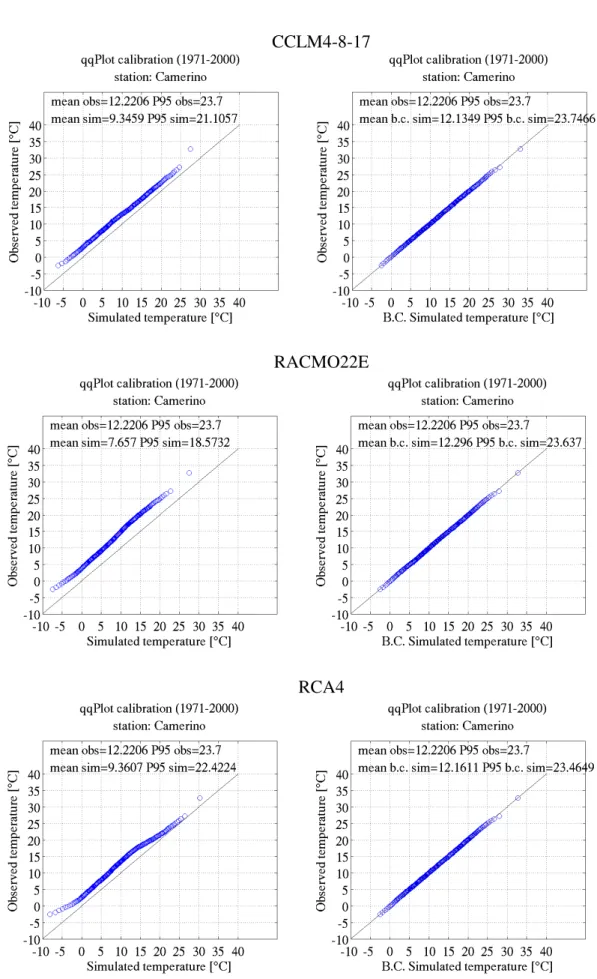
3.2.1 Quantile mapping bias correction ... 110

3.2.1.1 Correction function calibration – Temperature ... 111

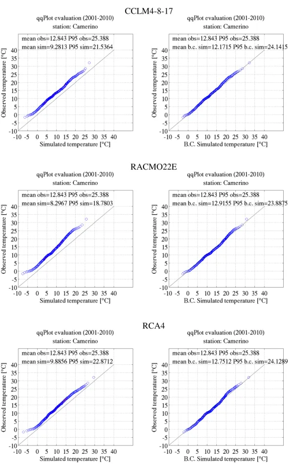
3.2.1.2 Correction function evaluation – Temperature ... 115

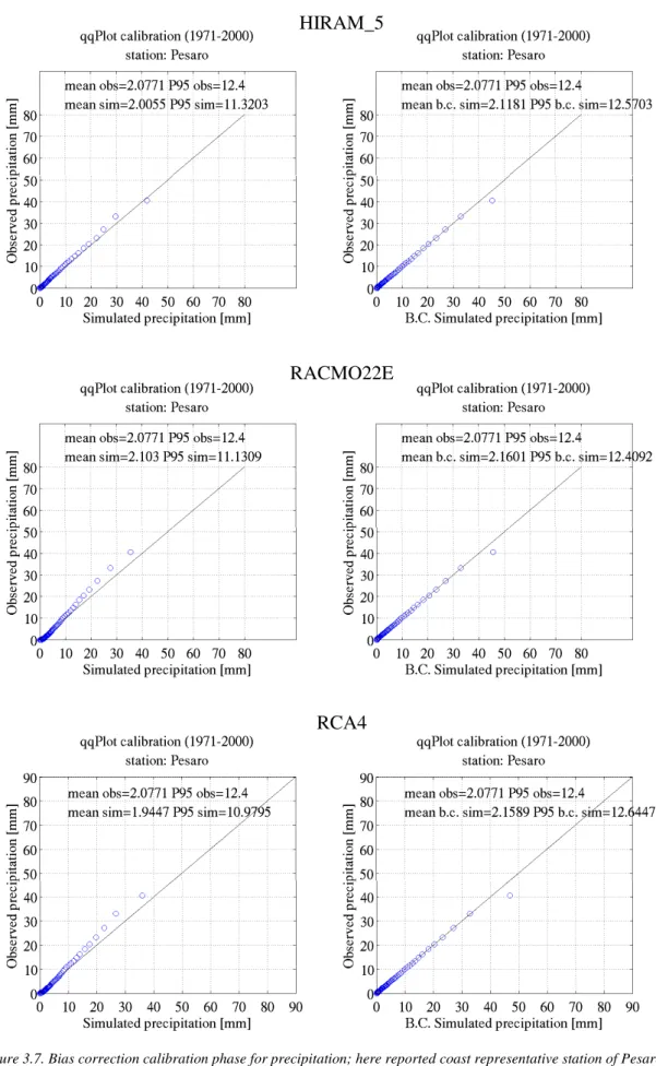
3.2.1.3 Correction function calibration – Precipitation ... 120

3.2.1.4 Correction function evaluation – Precipitation ... 124

3.2.2 Climate change signal and effect of bias correction – Temperature ... 128

3.2.2.1 Climate change signal annual cycle ... 128

3.2.2.2 Climate change signal distribution – Temperature ... 131

Mid-term scenario (2021-2050) – RCP4.5 ... 132

Long-term scenario (2061-2090) – RCP4.5 ... 134

3.2.2.3 Summary boxplots – Temperature ... 141

3.2.3 Climate change signal and effect of bias correction – Precipitation ... 149

3.2.3.1 Climate change signal annual cycle ... 149

3.2.3.2 Climate change signal statistical distribution – Precipitation ... 152

3.2.3.3 Summary boxplots - Precipitation ... 163

3.2.4 Changes of the hydrologic cycle in a warmer atmosphere: Hydro-climatic Intensity Index (HY-INT) ... 170

3.3 Conclusions and summary ... 175

3.3.1 Quantile mapping bias correction – Calibration phase ... 176

3.3.2 Quantile mapping bias correction – Evaluation phase ... 177

3.3.3 Climate change signal annual cycle ... 177

3.3.4 Climate change signal distribution ... 178

3.3.5 Local hydrologic cycle response to warmer atmosphere ... 179

(8)

(9)

Introduction

Why climate changes – short global warming history and principles

«Humanity is carrying out a wide-scale geophysical experiment never happened in the past and that cannot be reproduced in the future». This famous sentence formulated by Roger Revelle (1909-1991), published on «Tellus» journal, condensed in the half of 20th_century,

the essence of global warming issue. Revelle was not first scientist to postulate a potential atmosphere warming related to human activities. Greenhouse effect is being discussed since the half of 19th_{century, when Irish physicist John Tyndall (1820-1893) noted H}

2O and CO2

infrared absorption property and thus potentially important for climate in the 1861. Even, J. B. Fourier (1768-1830) theorized the analogy between warming effect of the atmosphere and a greenhouse in the 1827. However, one of the most relevant personality about theorization of global warming threat is represented by the Swedish chemist and physicist Svante August Arrhenius (1859-1927), which in the 1896 postulated the relation between climate change and CO2 as result of fossil fuels burning (at that time mainly coal). He provided a quantitative

description of the CO2 and water vapor in the thermal balance of the atmosphere, estimating

that a doubling of the CO2 concentration could lead to an increase of the global temperature

of roughly 4 °C (close to the results of modern climate model simulations). During the 20th

century and especially in the last thirty years new technologies including satellites, radar, telecommunication and supercomputing helped scientists to dramatically increase their understanding of climate system dynamics. In the 1988, was founded the Intergovernmental Panel on Climate Change (IPCC) as the result of concerted effort made by climate scientists to summarize the current state of knowledge. From then, IPCC reports represent recognized “center of gravity” concerning current climate science understanding. IPCC reports have the relevant role of making available to worldwide societies and policy makers best estimates of how global warming and related outcomes may evolve. The ability of producing improved climate information of the last three decades matched to a rising attention on making knowledge usable for all level society and on identifying best practices to do it. At this regard, «The Global Framework for Climate Services» implemented by the World Meteorological Organization in the 2009, attempts to identify a structure to support more informed decisions for saving lives, protecting the environment and assists economic

(10)

development coping with current and expected climatic changes (Vaughan and Dessai 2014). Climate services is a term come into favor fairly recent but it condenses thirty-years scientific effort for producing a flux of usable and tailored climate information for sectors as diverse as agriculture, health, water management and disaster risk reduction and for all the contexts that require climate information for their specific operations.

Climate change consists on “changes in climate conditions identified by statistical significant shifts on mean and/or variability of its properties, persisting for an extended period of decades or longer” (World Meteorological Organization (WMO); Intergovernmental Panel on Climate Change (IPCC), 2007). The United Nation Framework Convention on Climate change (UNFCCC, 2011) provides another definition of climate change: "a change of climate which is attributed directly or indirectly to human activity that alters the composition of the global atmosphere and which is in addition to natural climate variability observed over comparable time periods”. In the latter definition is present the key distinction between natural climate variability interacting (sharpening or dampening) with alteration ascribable to human activities.

Climate system is feed by the incoming solar radiation. This energy interacts with the Earth’s surface and with the atmosphere in order to achieve energetic equilibrium. The mean state of the atmosphere can be altered through internal processes and/or external forcing. Internal processes generate the intrinsic natural climate system variability present at all the time scale. Atmospheric processes relying internal variability operate on time scales ranging from instantaneous (condensation of water vapor in the clouds) to longer time scales involving complex interactions between climate components (atmosphere-hydrosphere-cryosphere-biosphere-land surface).

External influences, contributing to the climate variability, consist on processes influencing the level of solar radiation input (solar activity or Earth’s orbit configuration), and radiative processes which distribute solar energy between Earth and atmosphere. Solar radiation input is function of solar activity that, excluding paleoclimate variability, effects of are considered modest in recent climate changes and Earth’s orbit configuration. The latter, is estimated playing a relevant role on determining ice-age cycle. According to the M. Milankovitch (1879-1958) theory, incoming solar radiation would be influenced by orbital parameters such Earth’s orbit eccentricity, Earth’s axes inclination and the equinox precession cycles. However, only the former factor is considered relevant on influencing the

(11)

quantity of incoming solar radiation. Orbit eccentricity determines the level of seasonal variation regarding solar energy input (up to 30% during maximum eccentricity) varying on 100000 and 400000-year time scale.

The second external influence, involving radiative processes, is represented by natural phenomena such volcanism. These events consistently alter atmospheric reflectivity and consequently climate system energetic balance. Another source of radiative processes alteration is not natural and it is being taken place, since industrial revolution, strictly connected to anthropogenic activities (Hegerl et al. 2007).

Alterations regards the atmospheric chemical composition, through anthropogenic emission of radiatively important gasses (Greenhouse Gasses, GHGs), aerosols and by changing land surface properties. Longwave (or infrared) radiation, emitted from the Earth’s surface to balance solar radiation input, is consistently absorbed by atmospheric constituent GHGs (i.e. water vapor, carbon dioxide, methane, nitrous dioxide and other gasses) and clouds, which themselves emit longwave radiation in all directions. The downward component of this radiative emission increase heat in the lower layers of the atmosphere (Troposphere) and to the Earth’s surface. Additional warming of the surface determines higher upward infrared emission provoking further warming of the atmosphere. In this way recursive cycle has triggered, according to Stefan-Boltzmann low asserting that the energy released by a body (Hearth’s surface and atmosphere) is function of its temperature ( = ; where is the Stefan-Boltzmann constant). This is the greenhouse effect. In addition to GHGs concentration, Earth’s radiative balance is altered by aerosols. Depending on their chemical composition, concentration and lifetime can increase atmospheric reflectivity (enhancing albedo effect, indeed cooling effect) or conversely can act as strong solar radiation absorbers with a warming effect. Moreover, aerosols serve as clouds condensation. Clouds play a double role in climate system, increasing the albedo (cooling effect) but also warming through infrared downward emission. It depends on their altitude, physical properties and the chemical composition of cloud condensation nuclei. In general, cold clouds (cirrus) located roughly at 6000 m of altitude strength surface infrared emission blocking with a warming effect. Low-level clouds, with liquid content (stratus), reflect incoming solar radiation provoking cooling effect. Hence, it is of large interest identify which kind of clouds will be fostered by future climatic alterations. Human’s activities are not only altering atmospheric composition. Energy and water budgets are being altered as well by the changes of land surface properties. Conversion or burning forests to obtain

(12)

cultivable areas deeply affect carbon storage in the vegetation, adds CO2 and decreases

atmospheric CO2 extraction, reflectivity of land surface, and finally atmospheric water vapor

supply. All these factors, produce a radiative forcing, that represents a measure of the net change in the energy balance in response to an external perturbation. Once a forcing is applied, complex internal feedbacks determine the response of climate system general differing from a simple linear one. There are many mechanisms (feedback) in the climate system that can either amplify (‘positive feedbacks’) or diminish (‘negative feedbacks’) the effect of a certain change in climate forcing. An example of positive feedback is the reduction of ice albedo, where a decrease in the snow cover exposes darker underneath surface to absorb more solar radiation. Another positive feedback consists on methane release by several Earth’s surface or seafloor. Due to an increase of temperature, large Tundra and Arctic ecosystems of Asia and North-America are subjected to permafrost degradation. In such contexts, anaerobic decomposition of organic matter release massive methane emissions in to the atmosphere. The same happens in the oceans, where the increase of temperature produces release of seafloor-methane hydrates. An example of negative feedback could be represented by the increase in concentration of atmospheric aerosols with high level of reflectivity that enhance the atmospheric albedo effect.

These processes and many other alterations regarding fundamental aspects of biogeochemical cycles (e.g. Nitrogen cycle) and biological processes, are concurring on determining current shifts in global climate conditions.

How to predict future climate conditions - Climate projections

The current increase in GHGs concentration is considered virtually certain linked with observed alterations of the climate system (Myhre et al. 2013). Moreover, human influence on climate system is almost certain to continue in the near future (Hegerl et al. 2007). These evidences make societies increasingly demanding reliable projections of future climate change. Climate projections represent the basis for analyzing adaptation strategies, exploring mitigation measures and to support political decisions (Cubasch et al. 2013). Meanwhile knowledge of past and current climate variations is based on the statistical treatment of climate observations; future climate conditions description relies on the projections provided by climate models. World Meteorological Organization defines climate projections as the probability that certain climatic variation will take place in the next decades according to possible global socio-economic scenarios. In particular, to these scenarios correspond

(13)

particular future evolution of atmospheric GHGs concentration that affect future climate conditions. IPCC (2013) provides an updated climate projection definition consisting on an estimate of future climate conditions provided by climate models.

Basis for projections of future climate change are provided by climate models, describing the response of climate system to different radiative forcing from seasonal to decadal time scales (Stocker et al. 2010). Climate models are complex systems relying on a set of mathematical equations that are discretized on a grid and numerically solved on large computers (Knutti 2008). Mathematical equations describe the well-known physical principles (e.g. conservation of mass, energy, momentum, equation of state) that govern time derivative air masses motion and relation amongst variables at a given moment. Other processes occurring at scales smaller than the grid cell must be simplified and parameterized. For example, sub-grid processes that require parameterizations are the growing of trees, that modifying Earth’s surface can influence climate, or the treatment of moist convection and radiative transfer. For the part of the model governed by the fundamental physical lows computational capacity and thus higher resolution will improve the simulations. The term resolution is widespread used to describe the degree of refinement of a climate model grid. The increase of model resolution coupled to the increase of representation of smaller scale phenomena is roughly proportional to the computational time (and costs). Doubling the horizontal resolution of a climate models we double the operations that must be performed in calculating each term of each of the equation for each variable in each grid box. When horizontal resolution is increased, it is also necessary to proportionally reduce the time step to properly represent flux exchanges between one cell and the others. Conversely, for the part of the model solving empirical relation where no fundamental underlying lows exist the limiting factor are represented by human understanding of phenomena instead computational limits. Climate modeling has benefited from a variety of approaches to constructing climate models. In particular, benefits come from models that aim to simulate particular aspects of climate system, without attempting to include the full climate system complexity. A variety of climate models exists, guided by the different questions of interest developed to study different aspects of climate system components. Not always the most complicated model represent the best solution for that particular investigation being for instance not easy to interpret and too computational challenging (Knutti 2008). Indeed, it is possible to classify climate models in order of increasing complexity. Earth System Models are the current state-of-art models and they expand the Atmospheric-Ocean General Circulation Models

(14)

including description of various biogeochemical cycles such as Nitrogen cycle, Carbon cycle, Sulphur cycle, or Ozone (Flato et al. 2013). These represent the most comprehensive tools for simulating past and future response of climate system to various external forcing. Atmospheric-Ocean General Circulation Models (AOGCM) are considered standard climate models in climate change research. AOGCMs aim to represent physical component dynamics of climate system (atmosphere, ocean, land and sea-ice) and their response to future GHGs and aerosols forcing.

Regional Climate Models (RCMs) (Giorgi 1990), provide climate system representation comparable to that provided by AOGCMs, though generally run without interactive ocean and sea-ice. They are extensively used in climate for seasonal predictions to decadal climate projections. RCMs are characterized by higher resolution (10-50 km) and are the most common tool employed in regional climate research. Essentially, regional climate models simulate how global-scale climate change might affect individual region, reproducing effects of local topography over temperature and precipitation distribution patterns. Such models generate its small-scale climate response in function of the large-scale changes specified by the driving AOGCMs.

The RCMs higher resolution has obtained downscaling information belonging from the GCM. Since the 1990s RCMs have been constantly employed and improved, setting the basis to the tremendous development undergone by regional climate change studies in the last decade (Giorgi 2006a).

Producing regional climate projections

The remarkable development of regional climate change studies relies on a recognized evidence: is regional-to-local the spatial scale at which climate impacts act and have to be characterized. In climate change research, the term “regional” has a broad sense, indicating the entire range of spatial scale below the ≈ 10000 km2_{. Climate is globally changing but}

with highly heterogeneous temporal rate, spatial patterns and magnitude (Bindoff et al. 2013). Impacts of climate change are being observed to non-linearly respond to increase in temperature being function of particular ecological, cultural and socio-economic frame of human societies (Burke et al. 2015). In this context, regional climate information is necessary for assessing the impacts of climate changes over human and natural systems and develop mitigations and adaptation measures according to the different national level contexts (Giorgi et al. 2009). By the capability of providing solid and valuable regional-to-local scale

(15)

climate projections depends the tendency of end-user and policy makers to undertake mitigating and adaptive actions. Until the IPCC IV Assessment Report (2007), AOGCMs represented the main source of future climate information at global and sub-continental scale. Also with improved representation of many physical atmospheric and Earth surface processes, AOGCMs cannot capture effects of local forcing in function of the particular physiography and land-cover that deeply affect climate dynamics at the finer scales. AOGCMs coarse resolution is believed particularly limited on describing extreme events that are crucial information for the regional and local end-users (Giorgi et al. 2009). RCMs are indeed devoted to properly modulate the large-planetary-scale structure changes at regional (and in the best case local) scale according to the diversified local level (morphology, coastline physiography land-cover etc.) forcing.

To “regionalize” climate simulations provided by AOGCMs two principal methodologies (one dynamical and one statistical) exist. Concerning dynamical method, it could be discerned in two approaches. One approach, described by Giorgi (1990), implies different physical parameterizations in the nested (RCM) and driving model (GCM). Each parameterization is developed and optimized for the respective model resolution. This concept is known as one way nesting (Giorgi 1990). In the second approach (Laprise et al. 1998), the full physics of a GCM is implemented within a regional dynamical framework, and the regional model thus obtained is mostly run using driving conditions from the donor GCM. However, for regional climate modeling, basic point is the quality of forcing fields; good quality of these fields generally lead to improved quality of regional model experiment, regardless the means of these fields are obtained.

The second approach to downscale global climate information to more impact-suitable regional or local scale is represented by statistical downscaling. Statistical downscaling methodologies relying on the perfect prognosis principle (perfect prog. Wilks, 2011) have been considered for long time indicated technic tools for resolving the scale discrepancies between climate simulations and the resolution required for impact assessment (Maraun et al. 2010). Statistical downscaling establishes that local climate could be represented through a statistical model (transfer function) between large-scale observation/reanalysis data and local observation over present-day climate (Maraun et al. 2010; Themeßl et al. 2011b; Maraun et al. 2015). Applied directly to GCMs or RCMs for providing local climate scenarios, these statistical methods do not act on the correction of model outputs but only on refining spatial resolution. (Murphy 1999; Themeßl et al. 2011b). As seen for the dynamical

(16)

downscaling techniques, it could represent a drawback since systematic errors characterizing coarse-scale simulations could be passively inherit on the regional domain. This last concept let us introducing a relevant aspect connected with climate projections assessment referred as “climate projection uncertainties”.

Choice of downscaling method represents only one source concurring on the level of the intrinsic uncertainties affecting climate projections. Coherent interpretation and communication of climate projections uncertainties represent embedded processes in every future projections assessment, allowing end-users to evaluate consistencies of projected changes (Huard et al. 2014). In addition to downscaling approach, one of the most relevant uncertainty source regards “model configuration”. It is directly connected to the level of understanding of the physical processes which climate models are expected to reproduce. This kind of error can be directly propagate, if not amplified, from global to regional models (Giorgi et al. 2009). Other source of regional climate projection uncertainties is represented by the climate internal variability reproduction, mostly important in the short-term projection since could hide the presence of significant climate change signal (Hawkins and Sutton 2011). Frequently in climate change research multi-model ensemble approach, where several simulations averaged (arithmetically or weighted), is preferred. This approach leads to the production of a probabilistic climate change information (according to the number of ensemble member that produce same projection). Spread within of the multi-model ensemble could be used as explorative method of uncertainties. Finally, another source of uncertainty refers to the choice of future emission scenario providing radiative forcing boundary conditions to the climate simulations. It has been noted that the configuration of the driving AOGCM and the emission scenario uncertainties represent the two most relevant sources of uncertainty pertaining to regional climate projections, particularly at longer time-scale (Giorgi et al. 2009).

At European level, the most comprehensive research works based on regional-scale climate projections assessment are presented in PRUDENCE (Christensen and Christensen 2007), ENSEMBLES (van der Lindend and Mitchell 2009) and EURO-CORDEX (Jacob et al. 2013) projects. They are the reference European projects where a massive number of multi-RCM simulations and are produced, and employed in climate-impacts research. PRUDENCE project represents the first example where a wide number of climate projections have been employed in climate impacts studies as economy, agriculture and hydrology to depict a future impact scenario over these spheres (Déqué et al. 2005; Beniston et al. 2007;

(17)

Leander and Buishand 2007; Christensen and Christensen 2007). ENSEMBLES (van der Lindend and Mitchell 2009) represents a milestone of European climate change research. The research core of the project consists on providing multiple climate model runs (“ensembles”) providing a wide range of future projections assessed to define which more probable. This probabilistic information represents essential tool to assist society and policy makers in defining future measures to face climate change. Members of the project the most renowned European climate research centers (plus Canadian scientific consortium Ouranos). Each research institution contributed with its own simulations of the 20th and 21st century climate. CORDEX project has two-fold purpose, firstly providing a set of new high-resolution ensemble simulations for impact assessment and secondly to establish shared metrics for evaluating and benchmarking model performances (Giorgi et al. 2009; 2011; Vautard et al. 2013; Jacob et al. 2013; Kotlarski et al. 2014).

Italy, an interesting and challenging regional climate change case of study

As previously stated, climate is globally changing but with highly heterogeneous rate, spatial patterns and magnitude (Bindoff et al. 2013). Impacts of climate change are being observed to non-linearly respond to increase in temperature being function of particular ecological, cultural and socio-economic frame of human societies (Burke et al. 2015). For these reasons, changes in climate dynamics should be characterized as whole with exposure, vulnerability and adaptive-capacity characterizing each individual community. At this regard, Mediterranean basin, laying in unique geographical and transitional climate context has been identified as one of the world climate change Hot-Spot (Giorgi 2006b). Conceptually, a climate change Hot Spot, represents a region where coexist potential high impacts over the human-natural systems and a highly responsive climate to global change. (Giorgi 2006b). Lying at the center of Mediterranean basin, Italian peninsula, it is expected to be particularly susceptible to global climate change (Coppola and Giorgi 2010). Semi-arid conditions characterize southernmost regions, temperate conditions the central/northern sectors and cold climate characterizes Alpine area. Climate dynamics are deeply affected by the presence of the two major mountain chains Alps and Appennines respectively west-east and north-south oriented. Moreover, complex topography, high mountain and diverse coastline physiography make challenging to interpret local climate dynamics in response to the expected north-hemisphere major atmospheric modes alteration (Xoplaki et al. 2003; Xoplaki et al. 2004; Gaetani et al. 2011; Xoplaki et al. 2012; Bucchignani et al. 2015). For

(18)

these characteristics, Italian peninsula represents an interesting example of challenging climate-change case of study. Despite, comprehensive assessment of climate projections over Italia peninsula are still relatively sparse (Coppola and Giorgi 2010; Bucchignani et al. 2015; ISPRA 2015). According to expected changes affecting Mediterranean basin during the 21st_{century, Italian peninsula are expected to be affected by an exacerbation of the}

current warming and drying trends (Gao et al. 2006; Diffenbaugh et al. 2007; Hertig et al. 2010; Efthymiadis et al. 2011; Planton et al. 2012; Gualdi et al. 2013; Drobinski et al. 2014; Lionello et al. 2014). However, according to its high climate heterogeneity, relevant distinctions should be emphasized. As expected, change signal is in function of temporal horizon and the emission scenario considered but evident seasonal and latitudinal patterns also resulted (Giorgi 2006; Coppola and Giorgi 2010; Lionello 2012; Lionello et al. 2012). Moreover, several studies highlighted an asymmetry of temperature and precipitation distribution changes where extreme events are expected vary differently from the average. (Diffenbaugh et al. 2007; Fischer et al. 2007; Haarsma et al. 2009; Tolika et al. 2009; Hertig et al. 2010; Efthymiadis et al. 2011; Heinrich and Gobiet 2012). However, regarding future extreme events trend, many authors underline relevant uncertainties over magnitude and distribution patterns of expected changes. An example could be represented by the well-known climate models misrepresentation of complex dry-soil atmosphere feedbacks (Seneviratne et al. 2010; Orlowsky and Seneviratne 2011; Boberg and Christensen 2012) playing relevant role on determining length and magnitude of heat waves. At this regard, projected changes in inter-annual variability (oscillation of climate condition year-by-year) represent a good indicator on interpreting future temperature extreme trends. In Schär et al. (2004), was noted as future European summer climate might experience an increase in year-to-year variability, deeply affecting the incidence of heatwaves and drought. For precipitation, following thermodynamic and dynamic principles a generalized decrease of mean precipitation and an increase of extreme precipitation could be expected (Emori 2005; Palmer 2013; Coumou et al. 2014). However, especially for precipitation, identifying future dynamics and establishing a direct connection between increase in atmosphere temperature and extremes is anything but trivial (Frei and Schär 2001). Conversely, studies as Mariotti et al. (2008) and Senatore et al. (2011) highlight relevant consistency over expected changes in hydrologic cycle. Strong reduction of land-surface moisture availability is expected, where a significant decrease of main precipitation is coupled to an increase of winter evaporation (mainly over north-Italy) and a decrease of evaporation during summer (due to lower soil

(19)

moisture) over land. Concerning the Mediterranean Sea, precipitation reduction lower river run-off, warming-enhanced evaporation lead to a consistent loss in fresh water (Mariotti et al. 2008). These change patterns would be in agreement with the expected changes in the large-scale atmospheric modes with a north-ward expansion of the Hadley cell (Seidel et al. 2008; Planton et al. 2012) and increased positive phases of North Atlantic Oscillation (NAO) (Giorgi and Lionello 2008). The latter, substantially affects Atlantic storm track northward steering and cyclogenesis activity that regulate precipitation distribution in the whole Mediterranean region mainly in winter season (Giorgi and Lionello 2008; Xoplaki et al. 2012). For Italian peninsula, NAO positive phase means negative anomalies affecting winter precipitation. During this phase, compactness of polar vortex implicates higher-latitude Atlantic storm track. In turn, different studies stress how north-hemisphere large-scale circulation mode phases, are in turn influenced by the sea-ice extension and subsequently to the rate of its decline (Deser et al. 2010; Overland and Wang 2010). At this regard, Grassi et al. (2013) found evidences of increased NAO negative phase correlated to the reduction of winter sea-ice in correspondence of Barents-Kara sea region. NAO negative phase determines rippled sub-polar jet stream fostering low-pressure systems at the Mediterranean latitude. The same authors, referring to the Mediterranean region, indicate that even in the presence of general consistent increase of temperature cold spell will not disappear. Results indicated a tendency of increasing cold-rainy spells of winter precipitation over Italy with particular mention to the intense precipitation over the southern part of the Italian peninsula during winter season connected to a reduced extension of north-west Russian Arctic sea-ice. These highly diversified evidences stress the complexity of the large-scale dynamics interacting on defining Italian peninsula climate response to the anthropogenic forcing.

Bridging climate projections to climate impacts assessment

Intergovernmental Panel on Climate Change (IPCC) defines climate scenario as a “plausible representation of future climate that has been constructed for explicit use in investigating the potential impacts of anthropogenic climate change” (Mearns et al. 2001). Climate projections provided by climate models represent essential source of information for investigating the climate impacts for specific guesses about future human activities. However, alone, climate models projections do not provide sufficient information for defining future climate scenarios and related impacts to human and natural systems. Climate projections have to be properly managed and post-processed making them usable by climate

(20)

vulnerability, impacts and adaptation specialists. At this regard, the science of climate scenario provides the essential connection between climate simulations, produced by climate modelers and climate impact science. Several studies demonstrated that even newest generation of RCMs are still affected by systematic errors (Christensen et al. 2008; Boberg and Christensen 2012; Kotlarski et al. 2014). It complicates and deeply affects the capability of simulating and analyzing future climate impacts (Fowler et al. 2007). Hence, has been commonly established that some form of prior climate model outputs post-processing are strongly recommended before to use climate model outputs as inputs in impact modelling (Christensen et al. 2008).

Connection between climate model projections and climate impact research is particular delicate when local scale processes are considered (Smith et al. 2014). Local climate dynamics are the result of complex interactions between synoptic scale air mass motion, local morphology and orography. Even very high-resolution climate models (≈ 12 km) are limited in representing local climatology in complex physiography contexts. To be properly used in local impacts definition climate model outputs should be subjected to a double process devoted on the one hand to reduce model error (e.g. reduce discrepancies between meteorological observation and simulation over a common time segment) and on the other downscaled in order to include local climatology. As previously stated, statistical downscaling methodologies relying on the perfect prognosis principle (perfect prog. Wilks, 2011), have been considered for long time indicated technic tools for resolving the scale discrepancies between climate scenario and the resolution required for impact assessment (Maraun et al. 2010). Statistical downscaling establishes that local climate could be represent through a statistical model (transfer function) between large-scale observation/reanalysis data and local observation over present-day climate (Maraun et al. 2010; Themeßl et al. 2011b; Maraun et al. 2015). However, applied directly to GCMs or RCMs for providing local climate scenarios, these statistical methods do not act on the reduction of model output errors but only on refining spatial resolution. (Murphy 1999; Themeßl et al. 2011b).

Statistical post-processing bias correction according to the principle of Model Output Statistics (MOS; Wilks, 2011) may help to overcome this problem. In particular configurations, statistical bias correction techniques, couple RCM errors reduction to an improvement of the resolution at the same time (Themeßl et al. 2011b; Themeßl et al. 2011a; Casati et al. 2013; Smith et al. 2014). Statistical bias correction methods are indeed designed

(21)

to bridge the gap between climate model simulations and the climate data needed for quantitative assessment of climate impacts projections (Hempel et al. 2013).

Conceptually, bias correction methodologies aiming to reduce model errors could be discerned in two groups (Casati et al. 2013):

- Change factor methods that directly apply an average RCMs simulated climate change signal from future and present simulations to present climate observations. This method is widely called delta-change approach (Lenderink et al. 2007).

- Bias correction methods that rely on the relationship between present period observations and simulations to correct future model projections. In this context, the simplest approach corrects future climate simulation through a constant mean bias value characterizing simulations and observations during a present period. A drawback of this simple method is that error is considered constant over the whole statistical distribution consequently errors in variability are not corrected. Considering the future changes will differently affect mean values from high percentiles these technique could be considered too simplistic (Hagemann et al. 2011). Furthermore, given the high susceptibility of infrastructural and ecological systems to future extreme climatic events, it is suggestable to correct the entire statistical spectrum of climate model simulations. This could be performed through parametric (Piani et al. 2009; Piani et al. 2010) and non-parametric (empirical) bias correction methods (Boé et al. 2007; Deque 2007; Themeßl et al. 2011b; Themeßl et al. 2011a). A complete overview of statistical methodologies of bias correction is presented in Themeßl et al. (2011b), Berg et al. (2012) and Teutschbein and Seibert (2012) reporting comparison studies.

Amongst different approaches, empirical quantile mapping has been demonstrated to successfully remove systematic model errors due to high flexibility and high performance at high quantiles (Boé et al. 2007; Deque 2007; Themeßl et al. 2011b; Dosio and Paruolo 2011; Gudmundsson et al. 2012; Casati et al. 2013). In some particular configuration, such as employing in the correction finer grid or point scale observations, quantile mapping could help to bridge the gap between climate simulations and impact models resolution. In this case, bias correction performs error reduction and increase of simulation resolution (downscaling) at the same time also accounting for representativeness error (Casati et al. 2013). In fact, employing point-scale observations the discrepancies between observations

(22)

and simulations could result not only from intrinsic model error, but also from the spatial scale mismatch between model grid box and point-scale observations (Maraun et al. 2015). However, in climate change studies, it is not sufficient to prove bias correction efficacy on correcting recent or present climatology; of primary importance is also to characterize the effects of bias correction over the climate change signal (i.e. statistics difference between a future and past climate simulation). The influence of bias correction on future simulations and over climate change signal is only recently considered. (Scherrer et al. 2005; Dosio et al. 2012; Maurer and Pierce 2014; Gobiet et al. 2015). In Hagemann et al. (2011) and Haerter et al. (2011) has been observed that quantile mapping stretches the original climate change signal of a factor consistent with the ratio of observed and simulated standard deviation. Such modification of the original climate change signal is being strongly discussed and generally considered as deficiency of bias correction methods (Hempel et al. 2013). However, Maurer and Pierce (2014) argued that quantile mapping do not deteriorate the quality of climate change signal resulting from a multi-model ensemble experiment. Only recently has been provide an analytical demonstration (Gobiet et al. 2015) that regards this modification no more as a deficiency of bias correction but rather as an improvement of climate change signal. Analytical demonstration of Gobiet and colleagues (2015), relies on an intensity-dependence of model errors observed in several studies (Christensen et al. 2008; Themeßl et al. 2011a; Boberg and Christensen 2012). In these studies, has been noted a relationship between monthly mean temperature simulation errors and the observed monthly mean temperature with larger biases in warmer months than in colder months. Follows that where an error intensity-dependence exists climate change signal referred to warm months would be exaggerated. The effect of quantile mapping on climate change signal is mainly caused by the correction of the intensity-dependence of model error. That is, the effect should be seen as an improvement instead a drawback on the bias correction application in future climate change studies. However, considerations on improvement provided by quantile mapping relies on the postulate of a time-invariant model error characteristic. This means that the same processes misrepresented in present climate would be misrepresented even in the future climate simulation with similar bias associated to similar temperature. Since the correction function accounts for temperature-dependent biases, the future projections associated with those processes can be improved by quantile mapping. On the other hand quantile mapping cannot correct model errors generated by new physical processes that could occur in the future climate and not present in current dynamics (Casati et al. 2013). Maraun

(23)

(2012) in an experiment over Europe and employing ENSEMBLES project simulations found that in a transient climate change study biases are quite stable and bias correction on average improves the quality of climate scenario for climate impact studies.

Research pillars

Present work, according to different methodological approaches followed, could be discerned in three main pillars. First, a comprehensive regional climate projections assessment, roughly covering Italian peninsula is provided. In the second pillar, the same climate model outputs have been post-processed according to an empirical statistical bias correction. This second section is devoted to reduce the multi-model ensemble simulations error but without effects over the resolution of climate simulations since the correction function is built using equal resolution observed datasets. Third pillar takes a step further, shifting from regional to local-scale future climate scenario over representative Marche region (one of the 20 administrative divisions of Italy). Here same post-processing method was employed but built considering higher resolution ensemble simulations and point-scale observations. This configuration allows obtaining simulations error reduction coupled to spatial resolution increase.

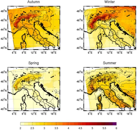
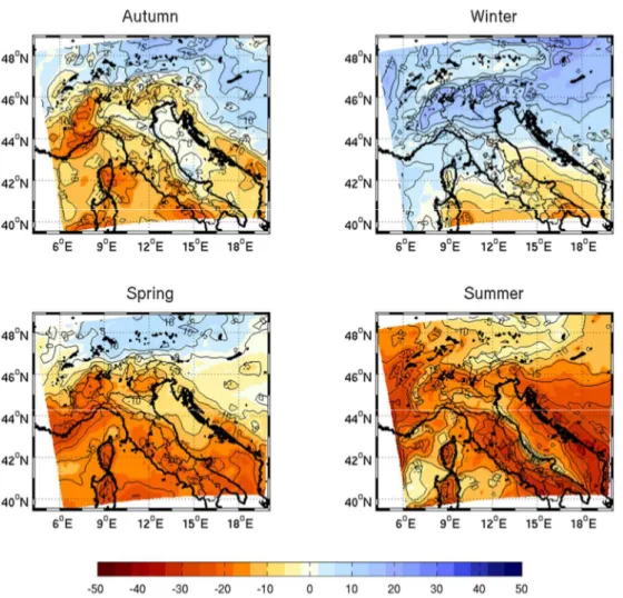
In the first pillar, a preliminary evaluation of the employed climate models through three statistical tests was performed. This section deals with the capability of the individual ensemble member to reproduce observed climatology of representative observational stations. Secondly, temperature and precipitation end-21st century climate change signal was analyzed. More in detail, considered variables are daily mean, minimum and maximum temperature and daily-cumulated precipitation. These key climate variable are the most used in climate change impact assessment studies (Giorgi et al. 2004). By definition, climate change signal is detected by comparing long-term statistics between a future (scenario) and past (reference) climate simulation (Mearns et al. 2001). Since changes are expected to differently affect mean value from high percentiles, different statistics signal have been considered. Furthermore, seasonal inter-annual temperature and precipitation variability response to increased radiative forcing was analyzed. Finally, operating with a multi-model ensemble approach, according to two different metrics, climate projections robustness and uncertainties were inspected.

(24)

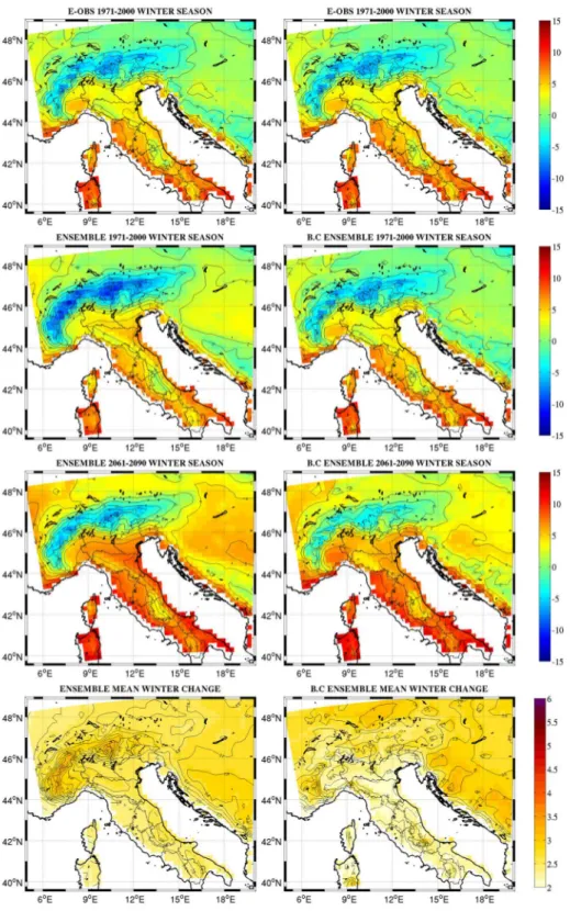
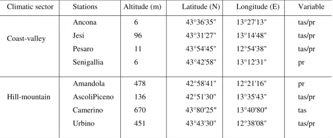
In the subsequent two pillars, two different spatial scale climate scenarios (one roughly covering Italian peninsula and the second focused over representative stations of Marche region) are built. In these sections, the focus is over the effect of the statistical bias correction on the climate change signal performed with original simulations. Indeed, discrepancies between original and bias-corrected results were assessed. While the statistical correction methodology is unvaried in the two experiments, substantial difference lies on the horizontal resolution of the simulations and observations employed. The first experiment (regional experiment) involves a regional dimension roughly covering Italian peninsula. Here, a multi-model ensemble (van der Lindend and Mitchell 2009), having a horizontal resolution of 25 km, is corrected employing an observational gridded dataset with the same horizontal resolution (Haylock et al. 2008). Given no spatial scale mismatch between simulation and observation, bias correction is expected to reduce simulation error with no effect on the resolution of climate simulations. This configuration has been chosen to avoid problems related to the representativeness error problems occurring where spatial scale mismatch between simulation and reference observation exists. Indeed, it is possible to isolate climate model errors generated by systematic model biases coupled to internal variability misrepresentation. Third pillar reports an experiment (local experiment) relying on higher resolution (12.5 km) multi model ensemble (Jacob et al. 2013) corrected with point-scale observational data. The observation are point-scale climatological time series provided by the observational network of Marche region Civil Protection. Given the spatial scale mismatch between simulations and observations, quantile mapping couples error reduction to the increase of climate projection resolution at the same time. Observational stations have been selected to represent the two main climatological sector of Marche region. A valley/coastal band belonging to “temperate sub-coastal” (pertaining to type “C” Koppen climate classification) climate classification characterized by temperature annual average between 10 °C and 14.4 °C. Rainfall are all year long distributed with a maximum in autumn (end-October - December) and a second relative maximum in spring (March – April). The overall annual precipitation are between 550-700 mm in the southern part (south of Ancona) and 700-800 (north of Ancona). The second climate sector considered corresponds to the hill-mountain regional areas. Here, the climate is defined “temperate-sub continental” with annual mean temperature enclosed between 10 °C and 14.4°C. The difference is in the minimum temperature of cold months (from -1 °C to +3.9 °C against from 4 °C to 5.9 °C).

(25)

Moreover, the periods characterized by mean temperature >= 20 °C are from 1 to 3 months against 3 months in sub-coastal bend. Annual precipitation between 750 to 1000 mm.

Finally, in the perspective of future climate change, Marche region, according to what observed by Giorgi and Coppola (2007) and Mariotti et al. (2008), is located on a particular transitional latitude. Concerning future winter precipitation climate change signal, the 2-degrees (from 42° N to 45° N) latitudinal band would be characterized by uncertain change sign (negative signal south of 42° N and a positive signal north of 45° N).

(26)

Bibliography

Beniston M, Stephenson DB, Christensen OB, Ferro C a T, Frei C, Goyette S, Halsnaes K, Holt T, Jylhä K, Koffi B, Palutikof J, Schöll R, Semmler T, Woth K (2007) Future extreme events in European climate: An exploration of regional climate model projections. Climatic Change 81:71–95. doi: 10.1007/s10584-006-9226-z

Berg P, Feldmann H, Panitz H-J (2012) Bias correction of high resolution regional climate model data. Journal of Hydrology 448-449:80–92. doi: 10.1016/j.jhydrol.2012.04.026 Bindoff N, Stott P, AchutaRao K, Allen M, Gillett N, Gutzler D, Hansingo K, Hegerl G, Hu

Y, Jain S, Mokhov I, Overland J, Perlwitz J, Sebbari R, Zhang X (2013) Detection and Attribution of Climate Change: from Global to Regional. Climate Change 2013: The Physical Science Basis Contribution of Working Group I to the Fifth Assessment Report of the Intergovenermnetal Panel on Climate Change 867–952.

Boberg F, Christensen JH (2012) Overestimation of Mediterranean summer temperature projections due to model deficiencies. Nature Climate Change 2:433–436. doi: 10.1038/nclimate1454

Boé J, Terray L, Habets F, Martin E (2007) Statistical and dynamical downscaling of the Seine basin climate for hydro-meteorological studies. 1655:1643–1655. doi: 10.1002/joc

Bucchignani E, Montesarchio M, Zollo AL, Mercogliano P (2015) High-resolution climate simulations with COSMO-CLM over Italy: performance evaluation and climate projections for the 21st century. International Journal of Climatology. doi: 10.1002/joc.4379

Burke M, Hsiang SM, Miguel E (2015) Global non-linear effect of temperature on Economic Production. Nature. doi: 10.1038/nature15725

Casati B, Yagouti A, Chaumont D (2013) Regional climate projections of extreme heat events in nine pilot Canadian communities for public health planning. Journal of Applied Meteorology and Climatology 52:2669–2698. doi: 10.1175/JAMC-D-12-0341.1

Christensen J, Kjellström E, Giorgi F, Lenderink G, Rummukainen M (2010) Weight assignment in regional climate models. Climate Research 44:179–194. doi: 10.3354/cr00916

(27)

Christensen JH, Boberg F, Christensen OB, Lucas-Picher P (2008) On the need for bias correction of regional climate change projections of temperature and precipitation. Geophysical Research Letters 35:L20709. doi: 10.1029/2008GL035694

Christensen JH, Christensen OB (2007) A summary of the PRUDENCE model projections of changes in European climate by the end of this century. Climatic Change 81:7–30. doi: 10.1007/s10584-006-9210-7

Coppola E, Giorgi F (2010) An assessment of temperature and precipitation change projections over Italy from recent global and regional climate model simulations. International Journal of Climatology 32:11–32. doi: 10.1002/joc

Coumou D, Petoukhov V, Rahmstorf S, Petri S, Schellnhuber HJ (2014) Quasi-resonant circulation regimes and hemispheric synchronization of extreme weather in boreal summer. Proceedings of the National Academy of Sciences. doi: 10.1073/pnas.1412797111

Cubasch U, Wuebbles D, Chen D, Facchini MC, Frame D, Mahowald N, Winther J-G (2013) Introduction In: Climate Change 2013: The Physical Science Basis. Contribution of Working Group I to the Fifth Assessment Report of the Intergovernmental Panel on Climate Change. Climate Change 2013: The Physical Science Basis Contribution of Working Group I to the Fifth Assessment Report of the Intergovernmental Panel on Climate Change 119–158. doi: 10.1017/CBO9781107415324.007

Deque M (2007) Frequency of precipitation and temperature extremes over France in an anthropogenic scenario: Model results and statistical correction according to observed values. Global and Planetary Change 57:16–26. doi: 10.1016/j.gloplacha.2006.11.030 Déqué M, Jones RG, Wild M, Giorgi F, Christensen JH, Hassell DC, Vidale PL, Rockel B,

Jacob D, Kjellström E, de Castro M, Kucharski F, van den Hurk B (2005) Global high resolution versus Limited Area Model climate change projections over Europe: Quantifying confidence level from PRUDENCE results. Climate Dynamics 25:653– 670. doi: 10.1007/s00382-005-0052-1

Deser C, Tomas R, Alexander M, Lawrence D (2010) The seasonal atmospheric response to projected Arctic sea ice loss in the late twenty-first century. Journal of Climate 23:333– 351. doi: 10.1175/2009JCLI3053.1

Diffenbaugh NS, Pal JS, Giorgi F, Gao X (2007) Heat stress intensification in the Mediterranean climate change hotspot. Geophysical Research Letters 34:1–6. doi: 10.1029/2007GL030000

(28)

Dosio a., Paruolo P (2011) Bias correction of the ENSEMBLES high-resolution climate change projections for use by impact models: Evaluation on the present climate. Journal of Geophysical Research 116:D16106. doi: 10.1029/2011JD015934

Dosio a., Paruolo P, Rojas R (2012) Bias correction of the ENSEMBLES high resolution climate change projections for use by impact models: Analysis of the climate change signal. Journal of Geophysical Research: Atmospheres 117:1–24. doi: 10.1029/2012JD017968

Drobinski P, Ducrocq V, Alpert P, Anagnostou E, Béranger K, Borga M, Braud I, Chanzy a., Davolio S, Delrieu G, Estournel C, Boubrahmi NF, Font J, Grubišić V, Gualdi S, Homar V, Ivančan-Picek B, Kottmeier C, Kotroni V, Lagouvardos K, Lionello P, Llasat MC, Ludwig W, Lutoff C, Mariotti a., Richard E, Romero R, Rotunno R, Roussot O, Ruin I, Somot S, Taupier-Letage I, Tintore J, Uijlenhoet R, Wernli H (2014) HyMeX: A 10-Year Multidisciplinary Program on the Mediterranean Water Cycle. Bulletin of the American Meteorological Society 95:1063–1082. doi: 10.1175/BAMS-D-12-00242.1

Efthymiadis D, Goodess CM, Jones PD (2011) Trends in Mediterranean gridded temperature extremes and large-scale circulation influences. Natural Hazards and Earth System Science 11:2199–2214. doi: 10.5194/nhess-11-2199-2011

Emori S (2005) Dynamic and thermodynamic changes in mean and extreme precipitation under changed climate. Geophysical Research Letters 32:L17706. doi: 10.1029/2005GL023272

Fischer EM, Seneviratne SI, Vidale PL, Lüthi D, Schär C (2007) Soil moisture-atmosphere interactions during the 2003 European summer heat wave. Journal of Climate 20:5081– 5099. doi: 10.1175/JCLI4288.1

Flato G, Marotzke J, Abiodun B, Braconnot P, Chou SC, Collins W, Cox P, Driouech F, Emori S, Eyring V, Forest C, Gleckler P, Guilyardi E, Jakob C, Kattsov V, Reason C, Rummukainen M (2013) Evaluation of Climate Models. Climate Change 2013: The Physical Science Basis Contribution of Working Group I to the Fifth Assessment Report of the Intergovernmental Panel on Climate Change 741–866. doi: 10.1017/CBO9781107415324

Fowler HJ, Blenkinsop S, Tebaldi C (2007) Linking climate change modelling to impacts studies : recent advances in downscaling techniques for hydrological. International Journal of Climatology 1578:1547–1578. doi: 10.1002/joc

(29)

Frei C, Schär C (2001) Detection Probability of Trends in Rare Events: Theory and Application to Heavy Precipitation in the Alpine Region. Journal of Climate 14:1568– 1584. doi: 10.1175/1520-0442

Gaetani M, Baldi M, Dalu G a., Maracchi G (2011) Jetstream and rainfall distribution in the Mediterranean region. Natural Hazards and Earth System Sciences 11:2469–2481. doi: 10.5194/nhess-11-2469-2011

Gao X, Pal JS, Giorgi F (2006) Projected changes in mean and extreme precipitation over the Mediterranean region from a high resolution double nested RCM simulation. Geophysical Research Letters 33:2–5. doi: 10.1029/2005GL024954

Gennaretti F, Sangelantoni L, Grenier P (2015) Toward daily climate scenarios for Canadian Arctic coastal zones with more realistic temperature-precipitation interdependence. Journal of Geophysical Research: Atmospheres 120, doi: 10.1002/2015JD023890 Giorgi F (2006a) Regional climate modeling: Status and perspectives. Journal de Physique

IV (Proceedings) 139:101–118. doi: 10.1051/jp4:2006139008

Giorgi F (2006b) Climate change hot-spots. Geophysical Research Letters 33:1–4. doi: 10.1029/2006GL025734

Giorgi F (1990) Simulation of regional climate using a limited area model nested in a general circulation model. Journal of Climate 3:941–963.

Giorgi F, Bi X, Pal J (2004) Mean, interannual variability and trends in a regional climate change experiment over Europe. II: Climate change scenarios (2071-2100). Climate Dynamics 23:839–858. doi: 10.1007/s00382-004-0467-0

Giorgi F, Jones C, Asrar GR (2009) Addressing climate information needs at the regional level : the CORDEX framework. WMO bulletin 58:175–183.

Giorgi F, Lionello P (2008) Climate change projections for the Mediterranean region. Global and Planetary Change 63:90–104. doi: 10.1016/j.gloplacha.2007.09.005

Gobiet a., Suklitsch M, Heinrich G (2015) The effect of empirical-statistical correction of intensity-dependent model errors on the climate change signal. Hydrology and Earth System Sciences Discussions 12:5671–5701. doi: 10.5194/hessd-12-5671-2015

Grassi B, Redaelli G, Visconti G (2013) Arctic sea ice reduction and extreme climate events over the mediterranean region. Journal of Climate 26:10101–10110. doi: 10.1175/JCLI-D-12-00697.1

Gualdi S, Somot S, Li L, Artale V, Adani M, Bellucci a., Braun a., Calmanti S, Carillo a., Dell’Aquila a., Déqué M, Dubois C, Elizalde a., Harzallah a., Jacob D, L’Hévéder B,

(30)

May W, Oddo P, Ruti P, Sanna a., Sannino G, Scoccimarro E, Sevault F, Navarra a. (2013) The CIRCE Simulations: Regional Climate Change Projections with Realistic Representation of the Mediterranean Sea. Bulletin of the American Meteorological Society 94:65–81. doi: 10.1175/BAMS-D-11-00136.1

Gudmundsson L, Bremnes JB, Haugen JE, Engen-Skaugen T (2012) Technical Note: Downscaling RCM precipitation to the station scale using statistical transformations - a comparison of methods. Hydrology and Earth System Sciences 16:3383–3390. doi: 10.5194/hess-16-3383-2012

Haarsma RJ, Selten F, Hurk B Vd, Hazeleger W, Wang X (2009) Drier Mediterranean soils due to greenhouse warming bring easterly winds over summertime central Europe. Geophysical Research Letters 36:1–7. doi: 10.1029/2008GL036617

Haerter JO, Hagemann S, Moseley C, Piani C (2011) Climate model bias correction and the role of timescales. Hydrology and Earth System Sciences 15:1065–1079. doi: 10.5194/hess-15-1065-2011

Hagemann S, Chen C, Haerter JO, Heinke J, Gerten D, Piani C (2011) Impact of a Statistical Bias Correction on the Projected Hydrological Changes Obtained from Three GCMs and Two Hydrology Models. Journal of Hydrometeorology 12:556–578. doi: 10.1175/2011JHM1336.1

Hawkins E, Sutton R (2011) The potential to narrow uncertainty in projections of regional precipitation change. Climate Dynamics 37:407–418. doi: 10.1007/s00382-010-0810-6

Haylock MR, Hofstra N, Klein Tank a. MG, Klok EJ, Jones PD, New M (2008) A European daily high-resolution gridded data set of surface temperature and precipitation for 1950-2006. Journal of Geophysical Research: Atmospheres. doi: 10.1029/2008JD010201 Hegerl GC, Zwiers FW, Braconnot P, Gillett NP, Luo Y, Orsini JAM, Nicholls N, Penner

JE, Stott P a (2007) Understanding and Attributing Climate Change. Climate Change 2007: The Physical Science Basis. Contribution of Working Group I to the Fourth Assessment Report of the Intergovernmental Panel on Climate Change. Cambridge University Press, Cambridge, United Kingdom and New York, NY, USA

Heinrich G, Gobiet A (2012) The future of dry and wet spells in Europe: A comprehensive study based on the ENSEMBLES regional climate models. International Journal of Climatology 32:1951–1970. doi: 10.1002/joc.2421

(31)

correction – The ISI-MIP approach. Earth System Dynamics 4:219–236. doi: 10.5194/esd-4-219-2013

Hertig E, Seubert S, Jacobeit J (2010) Temperature extremes in the Mediterranean area: Trends in the past and assessments for the future. Natural Hazards and Earth System Science 10:2039–2050. doi: 10.5194/nhess-10-2039-2010

Huard D, Chaumont D, Logan T, Sottile M-F, Brown RD, St-Denis BG, Grenier P, Braun M (2014) A Decade of Climate Scenarios – The Ouranos Consortium Modus Operandi. Bulletin of the American Meteorological Society 140116121450005. doi: 10.1175/BAMS-D-12-00163.1

ISPRA - Istituto Superiore per la Protezione e la Ricerca Ambientale (2015) Il clima futuro in Italia: analisi delle proiezioni dei modelli regionali

Jacob D, Petersen J, Eggert B, Alias A, Christensen OB, Bouwer LM, Braun A, Colette A, Déqué M, Georgievski G, Georgopoulou E, Gobiet A, Menut L, Nikulin G, Haensler A, Hempelmann N, Jones C, Keuler K, Kovats S, Kröner N, Kotlarski S, Kriegsmann A, Martin E, Meijgaard E, Moseley C, Pfeifer S, Preuschmann S, Radermacher C, Radtke K, Rechid D, Rounsevell M, Samuelsson P, Somot S, Soussana J-F, Teichmann C, Valentini R, Vautard R, Weber B, Yiou P (2013) EURO-CORDEX: new high-resolution climate change projections for European impact research. Regional Environmental Change 14:563–578. doi: 10.1007/s10113-013-0499-2

Knutti R (2008) Should we believe model predictions of future climate change? Philosophical transactions Series A, Mathematical, physical, and engineering sciences 366:4647–4664. doi: 10.1098/rsta.2008.0169

Kotlarski S, Keuler K, Christensen OB, Colette a., Déqué M, Gobiet a., Goergen K, Jacob D, Lüthi D, Van Meijgaard E, Nikulin G, Schär C, Teichmann C, Vautard R, Warrach-Sagi K, Wulfmeyer V (2014) Regional climate modeling on European scales: A joint standard evaluation of the EURO-CORDEX RCM ensemble. Geoscientific Model Development 7:1297–1333. doi: 10.5194/gmd-7-1297-2014

Laprise R, Caya D, Giguere M, Bergeron G, Côté H, Blanchet J, Boer GJ, McFarlane N a. (1998) Climate and climate change in western canada as simulated by the Canadian regional climate model. Atmosphere-Ocean 36:119–167. doi: 10.1080/07055900.1998.9649609

Leander R, Buishand TA (2007) Resampling of regional climate model output for the simulation of extreme river flows. Journal of Hydrology 332:487–496. doi:

(32)

10.1016/j.jhydrol.2006.08.006

Lenderink G, Buishand a., van Deursen W (2007) Estimates of future discharges of the river Rhine using two scenario methodologies: direct versus delta approach. Hydrology and Earth System Sciences 11:1145–1159. doi: 10.5194/hess-11-1145-2007

Lionello, P., Malanotte-Rizzoli, P., & Boscolo, R. (Eds.). (2006) Mediterranean climate variability (Vol. 4). Elsevier

Lionello P (2012) The Climate of the Mediterranean Region From the Past to the Future, 1st edn. Elsevier

Lionello P, Abrantes F, Congedi L, Dulac F, Gacic M, Gomis D, Goodess C, Hoff H, Kutiel H, Luterbacher J, Planton S, Reale M, Schröder K, Vittoria Struglia M, Toreti A, Tsimplis M, Ulbrich U, Xoplaki E (2012) Introduction: Mediterranean Climate— Background Information. The Climate of the Mediterranean Region xxxv–xc. doi: 10.1016/B978-0-12-416042-2.00012-4

Lionello P, Abrantes F, Gacic M, Planton S, Trigo R, Ulbrich U (2014) The climate of the Mediterranean region: research progress and climate change impacts. Regional Environmental Change. doi: 10.1007/s10113-014-0666-0

Maraun D (2012) Nonstationarities of regional climate model biases in European seasonal mean temperature and precipitation sums. Geophysical Research Letters 39:1–5. doi: 10.1029/2012GL051210

Maraun D, Wetterhall F, Ireson AM, Chandler RE, Kendon JE, Widmann M, Brienen S, Rust HW, Sauter T, Themeßl M, Venema VKC, Chun KP (2010) Precipitation Downscaling Under Climate Change : Recent Developments To Bridge the Gap Between Dynamical Models and the End User. Review of Geophysics 48:1–34. doi: 10.1029/2009RG000314.1

Maraun D, Widmann M, Gutierrez JM, Kotlarski S, Chandler RE, Hertig E, Wibig J, Huth R, Wilcke R a I (2015) VALUE: A framework to validate downscaling approaches for climate change studies. Earth’s Future 3:1–14. doi: 10.1002/2014EF000259

Mariotti A, Zeng N, Yoon J-H, Artale V, Navarra A, Alpert P, Li LZX (2008) Mediterranean water cycle changes: transition to drier 21st century conditions in observations and CMIP3 simulations. Environmental Research Letters 3:044001. doi: 10.1088/1748-9326/3/4/044001

Maurer EP, Pierce DW (2014) Bias correction can modify climate model simulated precipitation changes without adverse effect on the ensemble mean. Hydrology and