RIASSUNTO
La presente Tesi di Dottorato affronta lo studio delle tematiche relative al Project Management e al Project Scheduling sotto incertezza.
Il problema affrontato, che riveste un ruolo di notevole importanza sia dal punto di vista scientifico che dal punto di vista pratico, consiste nella determinazione di un piano temporale delle attività cositituenti un progetto (schedula), che tenga nel contempo conto della disponibilità limitata di risorse e della minimizzazione del tempo totale di completamento del progetto stesso (makespan).
La schedula di progetto definita sulla base di dati deterministici può essere soggetta a numerosi cambiamenti, in ragione del fatto che molteplici fonti di incertezza investono l’intero ciclo di vita del progetto.
La presente tesi si propone di fornire una serie di strumenti quantitativi, basati essenzialmente su framework della programmzaione stocastica, in grado di supportare la fase di pianificazione temporale di progetti soggetti ad incertezza. Nonostante il notevole interesse pratico ed applicativo della tematica affrontata, la letteratura scientifica riguardante il project scheduling sotto incertezza è ancora in fase embrionale. In particolare, risulta evidente la mancanza di una caratterizzazione probabilistica esplicita dell’incertezza e, come conseguenza, non vi è traccia di connesione di tale letteratura con l’ampio spettro di tecniche e metodi propri della branca della programmazione matematica sotto incertezza nota come programmazione stocastica.
La presente tesi offre un contributo innovativo in tale direzione, e si colloca pertanto nel quadro internazionale come il primo tentativo di affrontare la tematica del projet scheduling sotto incertezza con il framework della programmazione stocastica.
Nell’intraprendere lo studio di questa tematica nel Capitolo 3 si è ipotizzato che le risorse fossero comunque disponibili quando richieste, al fine di semplificare il problema e concentrare l’attenzione sulla gestione dell’incertezza.
In particolare il capitolo affronta il problema della caratterizzazione della funzione di distribuzione del makespan del progetto che, in condizioni di incertezza, può essere rappresentato da una variabile casuale con forma e caratteristiche non note.
Partendo dall’ipotesi che le durate delle attività costituenti il progetto siano variabili aleatorie la cui funzione di densità sia nota o possa essere stimata, sono stati proposti due metodi esatti per la soluzione del problema descritto.
L’efficienza dei due metodi propsti è stata poi testata su una batteria di problemi test tratti dalla letteratura e opportunamente modificati per tener conto dell’incertezza.
La ricerca svolta ha come caratteristiche distintive il superamento dell’approccio basato sul valore atteso su cui ad esempio il noto PERT si basa, contestualmente con l’introduzione di un’ottica avversa al rischio che ben si adatta alla gestione dei progetti in ambiti fortemente dinamici e competitivi. Inoltre, in modo originale rispetto alla letteratura, si è rilassata l’ipotesi di indipendenza delle durate delle attività, rappresentate come variabili aleatorie dipendenti con funzione di distribuzione discreta. L’originalità e la rilevanza dei risultati ottenuti è confermata dalla pubblicazione dei risultati della ricerca su rivista internazionale (Evaluating project completion time in project networks with discrete random activity durations- Computers & Operations Research 36(2009) 2716—2722).
Consolidati i concetti e le tecniche appresi in questa prima fase di studio, si è generalizzato il problema aggiungendo i vincoli sulle risorse.
Il problema in esame, noto in letteratura come Resource Constrained Project Scheduling problem –RCPSp- è stato oggetto di numerosi studi, finalizzati sia alla risoluzione del problema, nella sua versione deterministica.
Lo studio del problema in condizioni di incertezza (Robust Project scheduling ) ha portato alla definizione di approcci per la determinazione di schedule robuste, capaci cioè di assorbire gli effetti di eventuali “disruptions”, ossia di eventi capaci di modificare la durata e/o l’assorbimento di risorse delle attività del progetto. Con il termine “robustezza della soluzione” o “stabilità della schedula” ci si riferisce alla differenza tra la schedula di base e la schedula che si è effettivamente realizzata. Tale differenza rappresenta una misura della performance dell’algoritmo usato per la definizione della schedula di base: l’obiettivo da perseguire è in questo caso non la minimizzazione del makespan bensì la generazione di una soluzione che non venga deteriorata dal verificarsi di eventuali “disruptions” o eventi imprevisti.
Diversamente dai contributi presenti in letteratura, nel Capitolo 4 la robustezza della schedula è introdotta nel modello sotto forma di vincolo probabilistico, piuttosto che come misura da effettuare a posteriori con l’ausilio di tecniche di simulazione.
Per la risoluzione di tale problema è stata proposta una metodologia euristica che ha quale punto di forza l’uso di un modello che integra le comuni euristiche per lo scheduling dei progetti con strumenti propri della programmazione
stocastic. La metodologia proposta si pone come un’efficiente strumento di pianificazione da affiancare alle tradizionali procedure di pianificazione temporale dei progetti.
La validazione del modello proposto è stata operata attraverso un’ampia fase di sperimentazione, considerando quale misura di robustezza il “livello di confidenza” della schedula reale, cioè la probabilità che il makespan programmato rimanga tale almeno in misura pari a tale livello.
I risultati della ricerca hanno portato alla stesura di un articolo sottoposto a revisione internazionale ed attualmente in fase di terza revisione (A heuristic approach for resource constrained project scheduling with uncertain activity durations-sottomesso a Computers and Operations Research).
Infine, il Capitolo 5 presenta un caso reale di applicazione delle metodologie definite per la risoluzione dei problemi prima descritti, un progetto riguardante la costruzione di residenze per studenti universitari. L’obiettivo perseguito è consistito nella validazione di tale metodologia quale strumento efficace di pianificazione e gestione dell’incertezza nei progetti di costruzioni civili ed edili. La metodologia quantitativa applicata, è stata definita con l’obiettivo di ottenere una schedula quanto meno sensibile alle inevitabili perturbazioni nello svolgimento delle attività del progetto. L’applicazione di tale metodologia si è avvalsa di un DSS che ha permesso di identificare, analizzare e quantificare l'affidabilità della schedula definita e l'impatto su di essa di possibili eventi inattesi.
Siffatta metodologia si è quindi dimostrata più efficiente di quelle deterministiche comunemente usate, nello sfruttare le informazioni disponibili per fornire una pianificazione delle attività in condizioni di incertezza. Il valore aggiunto apportato da tale metodologia consiste nel rappresentare uno strumento in grado di supportare i manager nello sviluppo di una pianificazione delle attività progettuali efficace e realistica oltre a poter essere utilizzato come linea guida per il controllo e il monitoraggio dell’andamento del progetto. La ricerca condotta in questo Capitolo, ha portato alla stesura di un articolo accettato con revisioni minori in una rivista internazionale (A methodology for dealing with uncertainty in constructions projects-Engineering Computations).
Index
Chapter 1 _________________________________________________________ 9 Introduction _____________________________________________________ 9 1.1. The Resource Constrained Project Scheduling Problem –RCPSP- ________ 10 1.2. Uncertainty in project scheduling _________________________________ 10 1.3. Proactive VS Reactive project scheduling ___________________________ 11 Chapter 2 ________________________________________________________ 13
Definitions and Problem Formulation _______________________________ 13 2.1. Project representations _________________________________________ 13 2.1.1. Project network ___________________________________________ 14 2.1.2. Project Schedule __________________________________________ 15 2.1.2.1. Baseline schedule _______________________________________ 16 2.1.2.2. Realized schedule _______________________________________ 16 2.1.3. Resource usage and representations __________________________ 16 2.1.3.1. Resource profile ________________________________________ 17 2.1.3.2. Resource flow network___________________________________ 17 2.2. Robustness types and measures __________________________________ 19 2.2.1. Solution robustness or schedule stability ______________________ 20 2.2.2. Quality robustness ________________________________________ 20 Chapter 3 ________________________________________________________ 22
Project Scheduling Under Uncertainty Of Networks With Discrete Random Activity Durations _______________________________________________ 22
3.1. State of the Art ________________________________________________ 23 3.2. Model Proposal _______________________________________________ 23 3.3. Solution Methods ______________________________________________ 26 3.4. Computational Result __________________________________________ 31 Chapter 4 ________________________________________________________ 40 Resource Constrained Project Scheduling Under Uncertainty ____________ 40 4.1. Overview of the problem ________________________________________ 40 4.2. Stochastic project scheduling with robustness constraints _____________ 43 4.2.1. Notation and problem description ____________________________ 43
4.2.2. The heuristic procedure ____________________________________ 45 4.2.3. Generating activities completion times ________________________ 47 4.2.4. Solving the joint probabilistically constrained problem ___________ 50 4.3. Computational Experiments _____________________________________ 51 4.3.1. Benchmark approaches ____________________________________ 51 4.3.2. Computational results______________________________________ 52 4.3.3. Analysis of results _________________________________________ 54 4.3.3.1. Discrete distribution _____________________________________ 55 4.3.3.2. Continuous distribution __________________________________ 61 4.4. Conclusions __________________________________________________ 63 Chapter 5 ________________________________________________________ 69 A real application: Robust Project Scheduling in Construction Industry ____ 69 5.1. Introduction __________________________________________________ 70 5.2. Dealing with uncertainty in construction projects ____________________ 72 5.3. Empirical illustration of RAH: a real case study ______________________ 76 5.4. Analysys of Results _____________________________________________ 79 5.5. Conclusions __________________________________________________ 81 Appendix A ____________________________________________________ 83 Appendix B_____________________________________________________ 84 Appendix C _____________________________________________________ 86 Bibliography____________________________________________________ 87
List Of Figures and Tables
Table 1-1: Different methods for schedule generation under uncertainty ... 11
Figure 2-1: Example Project Network ... 15
Figure 2-2: A minimum duration schedule ... 15
Figure 2-3: Resource profile for example project ... 17
Figure 2-4: Resource flow network for the example project ... 18
Figure 2-5: Resource profile with resource allocation ... 19
Table 3-1: Test Problem Characteristics ... 31
Figure 3-1: Makespan-Reliability Trade-Off ... 33
Figure 3-2: Running time (in sec.) of AllPEA for the test problem j306 −10 as a function of the number of scenarios ... 33
Figure 3-3: Running time (in sec.) of SLPA for the test problem j306 −10 as a function of the number of scenarios ... 34
Figure 3-4: Influence of the order strength on AllPEA running time... 35
Figure 3-5: Influence of the order strength on SLPA running time ... 35
Figure 3-6: Computational time of AllPEA on different test problems ... 35
Figure 3-7: Computational time of SLPA on different test problems ... 36
Figure 3-8: Computational time trade-off between AllPEA and SLPA for test problem j1201 − 1 ... 37
Figure 3-9: Computational time trade-off between AllPEA and SLPA for test problem j601 – 1... 38
Figure 3-10: Computational time trade-off between AllPEA and SLPA for test problem N2, α = 0.99. ... 38
Figure 4-1: Toy example ... 48
Figure 4-2: Resulting schedule ... 49
Figure 4-3: values versus Tavg trade-off ... 56
Figure 0-1: Expected makespan for varying values-30 nodes-Discrete
case………57....53
Figure 0-6: Expected makespan for varying values-60 nodes-Discrete case………57....53
Figure 0-7: Expected makespan for varying values-90 nodes-Discrete case………57....54
Figure 0-8: Expected makespan components for varying values-30 nodes-Discrete case………57...
55 Figure 4.9: Davg for varying values-30 nodes-Discrete case……….55
Figure 4.10: Davg for varying values-60 nodes-Discrete case……….56
Figure 4.11: Davg for varying values-90 nodes-Discrete case……….56
Figure 4.12: Expected makespan for varying values-30 nodes-Continuous case…….……57
Figure 4.13: Expected makespan for varying values-60 nodes-Continuous case…….……57
Figure 4.14: Expected makespan for varying values90 nodes-Continuous case………..…57
Figure 4.15: TPCP for varying values-60 nodes-Continuous case………..59
Figure 4.16: TPCP for varying values-30 nodes-Continuous case………..59
Figure 4.17: TPCP for varying values-60 nodes-Continuous case………..59
Figure 4.17: TPCP for varying values-60 nodes-Continuous case………..60
Table 4-1: Results on 30 nodes test problems with discrete duration variability ... 64
Table 4-2: Results on 60 nodes test problems with discrete duration variability ... 65
Table 4-3: Results on 90 nodes test problems with discrete duration variability ... 66
Table 4-4: Results on 30 nodes test problems with continuous duration variability ... 66
Table 4-5: Results on 60 nodes test problems with continuous duration variability ... 67
Table 4-6: Results on 90 nodes test problems with continuous duration variability ... 67
Table 4-7: Average, minimum and maximum number of variables and constraints per iteration ... 68
Figure 5.1. Typical RAH iteration ... 74 Figura 5.2. Project network ... 77 Table 5-1: Activities ID, number, details, duration and resource requirement ... 78
Chapter 1
Introduction
The growing interest in the field of project management is confirmed by many new theories, techniques and computer applications designed to support project managers in achieving their objectives. Within project management, project scheduling aims to generate a feasible baseline schedule specifying, for each activity, the precedence and resource feasible start times used as a baseline for project execution. Baseline schedule helps manager to visualize project evolution, giving a starting point for both internal and external planning and communication.
Careful project scheduling has been shown to be a key factor to improve the success rate of the project. A recent study by Maes et al. (2000) has found that inferior planning is the third reason of company failure in the Belgian construction industry. This struggles researchers to further develop new project scheduling methods.
After the concepts of project management and project scheduling have been introduced, in the next section the standard problems in project scheduling will be shortly presented followed by a brief introduction of concepts of stable project scheduling.
1.1. The Resource Constrained Project Scheduling
Problem –RCPSP-
The Resource Constrained Project Scheduling problem aims at minimizing the duration of a project subject to precedence and resource constrains in a deterministic environment. Precedence constrains are assumed belonging to the best-known type of precedence relationships, the finish-start zero-lag relationship. Subject to such type of constrains, each activity is forced to start when all its predecessors have been completed. As far as resources are concerned, we limit our dissertation on renewable resource constraints, assuming resources available on a period-by-period basis and for which only the total resource use in each time period is constrained for each resource type.
Many exact and heuristic algorithms have been described in the literature to construct workable baseline schedules that solve the deterministic RCPSp, that has been shown to be NP-Hard in a strong sense. For extensive overviews we refer to Herroelen et al. (1998), Kolisch & Padman (1999), Kolisch & Hartmann (1999), Brucker et al. (1999) and Demeulemeester & Herroelen (2002).
1.2. Uncertainty in project scheduling
In a real life context, project execution is subject to a considerable uncertainty. Uncertainty can originate from multiple source: resources can become temporarily unavailable (Lambrechts et al. 2007,2008) and Drezet 2005), activities may have to be inserted or dropped (Artigues & Roubellat 2000), due dates may change, activities may take longer or less long than original expected, etc. As a consequence, although usefulness of baseline schedule is unquestionable, project will never execute exactly as it was planned due to uncertainty. The common practice of dealing with these uncertainties by taking deterministic averages of the estimated parameters might lead to serious fallacies (Elmaghraby 2005).
When duration of activities is assumed stochastic, we move to the field of stochastic RCPSp. A solution for the stochastic RCPSP needs to define the
appropriate reactive action for every possible disruptive event during project execution, given the current state of the project and the a priori knowledge of future activity distributions. Möhring et al. (1984, 1985) call such a reactive way of generating a solution a scheduling policy or
scheduling strategy: a policy makes dynamic scheduling decisions during
project execution at stochastic decision points, usually corresponding to the completion times of activities. In pure dynamic scheduling (Stork 2001), the use of schedules is even eliminated altogether.
The absence of a schedule has some consequences from an economic point of view. The baseline schedule (pre-schedule, predictive schedule) namely serves a number of important functions (Aytug et al. 2005), Mehta & Uzsoy 1998), such as facilitating resource allocation, providing a basis for planning external activities (i.e. contracts with subcontractors) and visualizing future work for employees. The baseline schedule needs to be sought before the beginning of the project as a prediction of how the project is expected to unfold. It has been observed, (Yang 1996), that using the baseline schedule together with a dispatching rule, i.e. proactive-reactive
scheduling detailed in the following paragraph, often leads to a lower
expected makespan than pure dynamic scheduling procedures. The following table distinguishes between three basic approaches for the development of a baseline schedule (Herroelen & Leus 2005).
Baseline schedule During project execution (i) No baseline schedule
(ii) Baseline scheduling with no anticipation of variability
(iii) Baseline scheduling with anticipation of variability
(i) Dynamic scheduling (scheduling policies)
(ii) Reactive scheduling
(iii) Proactive (robust) scheduling
Table 1-1: Different methods for schedule generation under uncertainty
1.3. Proactive VS Reactive project scheduling
In general, there are two approaches to deal with uncertainty in a scheduling environment (Davenport and Beck 2002; Herroelen & Leus 2005): proactive and reactive scheduling.
Proactive scheduling constructs a predictive schedule that accounts for
statistical knowledge of uncertainty. The consideration of uncertainty information is used to make the predictive schedule more robust, i.e., insensitive to disruptions. Reactive scheduling involves revising or reoptimizing a schedule when an unexpected event occurs. At one extreme, reactive scheduling may not be based on a predictive schedule at all: allocation and scheduling decisions take place dynamically in order to account for disruptions as they occur. A less extreme approach is to reschedule when schedule breakage occurs, either by completely regenerating a new schedule or by repairing an existing predictive schedule to take into account the current state of the system.
It should be observed that a proactive technique will always require a reactive component to deal with schedule disruptions that cannot be absorbed by the baseline schedule. The number of interventions of the reactive component is inversely proportional to the robustness of the predictive baseline schedule. Many different types of robustness have been identified in the literature.
In the next chapter, notations and definitions will be provided to formally describe the problem that will be tackled in the remaining chapters.
Chapter 2
Definitions and Problem
Formulation
In this chapter, a definition of the proactive project scheduling problem is given. Section 2.1 introduces project representations that help us in illustrating the procedures that will be proposed in later chapters. Afterwards, we propose a rigorous definition of the concepts of quality and solution robustness, which both will be main issues throughout this thesis (Section 2.2).
2.1. Project representations
A project consists of a number of events and activities or tasks that have to be performed in accordance with a set of precedence and resource constraints. The deterministic expected duration of activity j will be expressed as dj, while in an uncertain scheduling environment, the stochastic activity durations will be denoted by dj. The activity-dependent weights used in this dissertation represent the marginal cost of starting the activity j later or earlier than planned in the baseline schedule. Once a project schedule has been negotiated, constructed and announced to all stakeholders, modifying this schedule comes at a certain penalty cost. This cost corresponds to the importance of on-time performance of a task to avoid internal and external stability costs. Internal stability costs for the
organization may include unforeseen storage costs, extra organizational costs or just a cost that expresses the dissatisfaction of employees with schedule nervousness. Costs related to (renegotiating) agreements with subcontractors, penalty clauses, goodwill damages, etc. are examples of stability costs that are external to the organization.
2.1.1. Project network
A project network is a graphical representation of the events, activities and precedence relations of the project. A network is a directed graph G = (N,A), consisting of a set of nodes N={0,..,N} and a set of arcs A. The transitive closure of a graph G = (N,A) is a graph TG = (N, TA) which contains an edge from i to j whenever there is a directed path from i to j in the original graph. The main focus of the project network is the representation of the precedence relationships between the activities of the project.
There are two network notation schemes commonly used in project scheduling. The activity-on-arc (AoA) representation uses the set of nodes
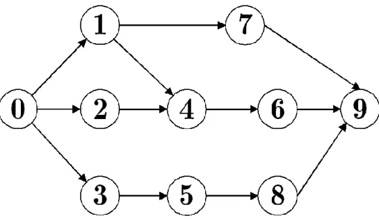
N to represent events and the set of arcs A to represent the activities, while in the activity-on-node (AoN) notation scheme, the set N denotes the activities and the set A represents the precedence relationships. The arcs TA of the transitive closure TG = (N, TA) represent in this case all direct and transitive precedence relationships in the original network. Now we introduce a project that will be used as our vehicle for definition and problem formulation. Let consider a project consisting of 10 activities (activity 0 and activity 9 are dummy activities representing the project start and finish) subject to finish-start, zero-lag precedence constraints and a single renewable resource constraint. The single renewable resource is assumed to have a constant per period availability a of 10 units. Expected activity durations dj , activity weights wj and resource requirements are also given. Figure 2.1 denotes the AoN project network for the project described in Table 2.1.
Figure 2-1: Example Project Network
2.1.2. Project Schedule
A schedule S is defined in project scheduling as a list S = (s0, s1, . . . , sn) of intended start times sj≥ 0 for all activities j N. A Gantt chart (introduced by H. Gantt in 1910) provides a typical graphical schedule representation by drawing the activities on a time axis.
A schedule is called feasible if the assigned activity start times respect the constraints imposed on the problem. In deterministic project scheduling, a feasible schedule is a sufficient representation of a solution.
Figure 2-2: A minimum duration schedule
2.1.2.1. Baseline schedule
A baseline schedule (pre-schedule or predictive schedule) is a list of activity start times generated under the assumption of a static and deterministic environment that is used as a baseline during actual project execution. A baseline schedule is generated before the actual start of the project (time
0) and will consequently be referred to as S0.
It serves a number of important functions (Aytug et al. (2005), Mehta & Uzsoy (1998), Wu et al. (1993)). One of them is to provide visibility within the organization of the time windows that are reserved for executing activities in order to reflect the requirements for the key staff, equipment and other resources. The baseline schedule is also the starting point for communication and coordination with external entities in the company’s inbound and outbound supply chain: it constitutes the basis for agreements with suppliers and subcontractors (e.g. for planning external activities such as material procurement and preventive maintenance), as well as for commitments to customers (delivery dates).
2.1.2.2. Realized schedule
A realized schedule ST is a list of actually realized activity start times ST that is generated once complete information of the project is gained.
The proactive-reactive scheduling decisions made during project execution influence the actually obtained realized schedule ST. In a stochastic environment, the realized schedule will thus typically be unknown before the project completion time T. We will refer to this stochastic schedule by ST.
2.1.3. Resource usage and representations
In resource-constrained project scheduling, project activities require resources to guarantee their execution. Multiple resource categories exist (Blazewicz et al. 1986) but in this thesis (as in the RCPSP), we will limit our scope to renewable resources that are available on a period-by-period basis and for which only the total resource use in each time period is constrained for each resource type.
Every activity j requires an integer per period amount rjk of one or more renewable resource types k (k = 1, 2, ...,K) during its execution. The renewable resources have a constant per period availability ak. The
resource constraints can thus be written as:
in which Pt denotes the set of activities that are active at time t.
The network (see Section 2.1.1) and schedule (see Section 2.1.2) representations of the project do not visualize the resource allocation. Hence, additional resource-based project representations are introduced in this section.
2.1.3.1. Resource profile
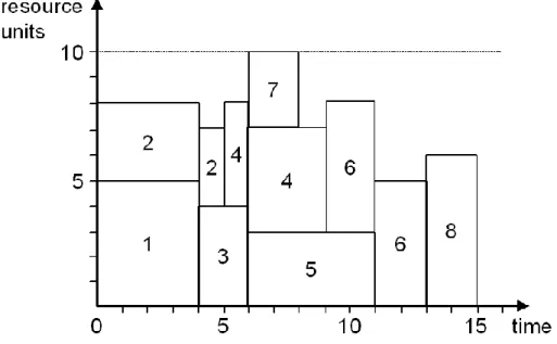
A resource profile is an extension of a Gantt chart that additionally indicates the variation in resource requirement of a single renewable resource type over time for each activity. Resource requirements and availability are denoted on the Y-axis. Each resource type requires its own resource profile. The resource profile for the single renewable resource type corresponding to the minimum duration schedule of Figure 2.2 is given in Figure 2.3.
Figure 2-3: Resource profile for example project
2.1.3.2. Resource flow network
Artigues et al. (2003) define resource flow networks (or transportation
one activity to the beginning of another activity after scheduling has taken place. fijk denotes the amount of resources of type k, flowing from activity i
to activity j. The resource flow network is a network with the same nodes N as the original project network, but with arcs connecting two nodes if there is a resource flow between the corresponding activities, i.e.
We define R as the set of flow carrying arcs in the resource flow network. The resource arcs in R may induce extra temporal constraints to the project. We remark that a schedule may allow for different ways of allocating the resources so that the same schedule may give rise to different resource flow networks. Not every feasible resource allocation implies an equal amount of stability.
Relying on the one-pass algorithm of Artigues et al. (2003) to compose a resource flow network for the schedule of Figure 2.2, results in the resource flow network G = (N,R) presented in Figure 2.4. Activity 8, for example, has a per period resource requirement of six units. It uses three resource units released by its predecessor activity 5, two units passed on by activity 7 and one unit released by activity 6. The arcs (1,3); (3,7); (6,8), (7,6) and (7,8) represent extra precedence relations that were not present in the original network. The arc (7,9) was present in A, but is not drawn in Figure 2.4 because there is no resource flow from 7 to 9.
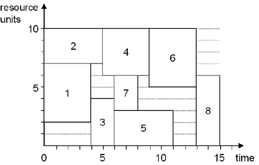
In the following figure, -Figure 2.5-, the resource profile of Figure 2.3 is reported to illustrate the use of the individual resource units along the horizontal bands. This project representation includes both the resource profile and the resource flow network and will thus become our preferred representation in the remainder of this dissertation if there is only one resource type, as is the case in the example network.
Figure 2-5: Resource profile with resource allocation
2.2. Robustness types and measures
In Chapter 1, the concept of schedule robustness was mentioned as a schedule’s insensitivity to disruptions that may occur during project execution. Many different types of robustness have been identified in the literature, calling for rigorous robustness definitions and the use of proper robustness measures. Two often used types of single robustness measures have been distinguished: solution and quality robustness (Sörensen (2001), Herroelen & Leus (2005)). The main difference between quality robustness and solution robustness is that in the former case, it is the quality of the solution that is not allowed to change. This quality is usually measured in terms of makespan or due date performance.
2.2.1. Solution robustness or schedule stability
Solution robustness or schedule stability refers to the difference between the baseline schedule and the realized schedule. The difference or distance (S0, ST) between the baseline schedule S0 and the realized schedule ST for a
given execution scenario can be measured as the number of disrupted activities, the difference between the planned and realized activity start times, and other different ways.
For example, the difference can be measured by the weighted sum of the absolute deviation between the planned and realized activity start times:
where denotes the planned starting time of activity j in the baseline schedule S0, denotes the actual starting time of activity j in the realized
schedule ST , and the weights wj represent the disruption cost of activity j
per time unit, i.e. the non-negative cost per unit time overrun or underrun on the start time of activity j.
In a stochastic environment, the realized activity starting times are stochastic variables for which the actual realized values for a given execution scenario depend on the disruptions and the applied reactive policy. The objective of the proactive-reactive scheduling procedure is then
to minimize:
with E denoting the expectation operator, i.e. to minimize the weighted sum of the expected absolute difference between the planned and the realized activity start times.
2.2.2. Quality robustness
Quality robustness refers to the insensitivity of some deterministic objective value of the baseline schedule to distortions. The goal is to generate a solution for which the objective function value does not deteriorate when disruptions occur. Contrary to solution robustness, quality robustness is not concerned with the solution itself, only with its value on the performance metric. It is measured in terms of the value of some objective function z. In a project setting, commonly used objective functions are project duration (makespan), project earliness and tardiness, project cost, net present value,etc.
When stochastic data are available, quality robustness can be measured by considering the expected value of the objective function, such as the expected makespan E [Cmax], the classical objective function used in stochastic resource-constrained project scheduling (Stork 2001).
It is logical to use the service level as a quality robustness measure, i.e. to maximize P(z ≤ z), the probability that the objective function value of the realized schedule stays within a certain threshold z. For the makespan objective, we want to maximize the probability that the project completion time does not exceed the project due date n), where is a stochastic variable that denotes the starting time of the dummy end activity in the realized schedule. We will refer to this measure as the timely project completion probability (TPCP). It should be observed that also the analytic evaluation of this measure is very troublesome in the presence of ample resource availabilities. In the next chapter we introduce a new heuristic approach with the aim to evaluate project completion time with discrete random activity durations.
Chapter 3
Project Scheduling Under
Uncertainty Of Networks With
Discrete Random Activity
Durations
In real projects, defining a good schedule on the basis of deterministic processing times is usually inadequate, because these times are only estimates and are susceptible to unpredictable changes. Deterministic models for project scheduling suffer from the fact that they assume complete information and neglect random influences, that occur during project execution. A typical consequence is the underestimation of the project duration as frequently observed in practice, even in the absence of resource constraints.
In this chapter a method for obtaining relevant information about the project makespan for scheduling models, with dependent random processing time available in the form of scenarios and in the absence of resource constraints is presented.
3.1. State of the Art
As previously discussed, real projects are subject to considerable uncertainty due to a number of possible sources. Resources may become unavailable, activities duration may experience some delay, new activities may be incorporated in the project or other activities may be even deleted. Amongst the full range of sources of significant uncertainty associated with any given project (Atkinson et al. 2006), an obvious aspect of uncertainty concerns estimates of potential variability of activity duration. In this context, our choice involves modeling processing times of activities as random variables. A very traditional issue with respect to stochastic networks is the derivation of the distribution or quantiles of the project completion time. This issue may be valuable in project management, particularly at the time of bidding, and has been the subject of investigation within both academia and industry. A great deal of research has been carried out on methodologies for estimating project time distributions. Due to the inherent difficulty of this task, two main distinct methodologies have been applied, that is the simulation approach (Van Slyke (1963), Sullivan & Hayya (1980), Herrera (2006), Shih (2005)) and the analytical approach (Dodin (1985), Hagstrom, (1990)).
Other approaches focus on approximating either the expected completion time value (Fulkerson 1962) or the probability for completing the project within a given deadline (Soroush 1994) as tightly as possible. A comprehensive review of most of the earliest references is presented in (Elmaghraby 1989). For more recent results the reader is referred to Yao and Chu (2007) and references therein. Hagstrom (1988) showed that the problem of computing the probability that a project finishes by a given time, when activities durations are discrete, independent random variables, is NP-complete.
3.2. Model Proposal
We now present an efficient method to find quantiles of the distribution function when activities durations are dependent discrete random variables, or when a suitable discretization in the form of scenarios is available for continuous dependent random variables. The output can be used by a
contractor to assess its capabilities to meet the contractual requirement before bidding and to quantify the risks involved in the schedule.
In this case, the specification of a project is assumed to be given in activity-on-arc (AoA) notation by a connected, directed acyclic graph G(N,A) (referred to as project network), in which N is the set of nodes, representing network “events”, and A is the set of arcs, representing network activities. We assume that there is a single start node 0 and a single terminal node n. When the durations of all the activities are constants, project managers may easily calculate the project completion time by the well-known critical path method. Let denote by
the set of paths from the node 0 to the node n in G(N,A). The project makespan can obviously be defined as
where represents the length of the path from node 0 to node n. Suppose now that we want to estimate the project duration that will not be exceed with probability at least α, that is, we want to estimate the α-quantile of the makespan distribution function. This information can be obtained through the solution of the following problem:
(1)
(2) (3)
where represents the start time of event i and is the random variable associated to the length of the path from the start node 0 to the terminal node n. We consider the starting time of node 0 equal to zero.
The - quantiles of the makespan represents a project duration that, with a probability α, will not be exceeded. In fact, the joint probabilistic constraints assures that
with probability at least α.
This definition allows to address the decision-makers risk aversion, ensuring that the project’s operations are unaffected by major delays with a high level of probability.
It is well known that the expectation criterion of the classical PERT model (Malcolm et al. 1959) is most appropriate for a risk-neutral decision maker. We trivially observe that reasoning on the basis of averages always results in an underestimate of the expected duration of the project and leads to a probability of exceeding the due date of the project near to 50%. Criticism against the use of averages has been raised in (Elmaghraby 2005), where a demonstration that gross errors can be made using the average as optimization criterion is reported.
In order to account for possible risk averseness we use the joint probabilistic constraints (2). Such conservatism should be invoked when large potential gains and losses are associated with individual decisions (Schuyler 2001).
It is worth while observing that the use of individual probabilistic constraints is not suitable for this problem, since will normally be dependent even if the random arc weights are independent, because of common arcs.
Therefore, we consider a formulation with joint probabilistic constraints involving dependent random right-hand side variables. This probabilistic constrained framework is well suited for this kind of problem and it is particularly useful when the penalty for the project to be completed late is very high or simply is not easily quantifiable. The use of chance constrained programming methods to examine some statistical properties of stochastic networks, is not completely new.
Charnes et al. (1964) considered the following chance constrained model to characterize the distribution of total project completion time:
(4)
(5) (6)
However we notice that the chance constraints paradigm is used, regardless the dependency among activities and paths, and in addition, since the stochastic precedence constraints are written in terms of the starting time of the preceding events, a dynamic problem is established, for which the use of a static stochastic programming problem should be prevented.
The developed model differs from other approaches proposed in the literature in several aspects.
• The methodology does not require any hypothesis on the distribution function of the activities durations. We only assume that a probability density function has been specified for each activity time and that a suitable discretization is available. Different distributions can be used to model different activity times.
• Our model overcomes the limitation of stochastic independence among activities times. Often activities durations are correlated trough the common usage of resources or precedence relations.
• Our model overcomes the limitation of stochastic independence among the paths of the network. Paths are in fact correlated via common activities and the correlation is treated explicitly in the use of joint probabilistic constraints
• Unlike sensitivity analysis, we can account for the effects of simultaneous changes to multiple activity times.
• In the proposed model, by varying the reliability threshold, decision makers might acquire information about different alternatives and might choose the maximum probability of violating the project due date which is allowed to be tolerated.
Finally, we would like to remark that the probabilistic paradigm is one of the most powerful prescriptive methodologies for decision makers, in that represents the global probability of violation of the constraints. Clearly, the most appropriate paradigm for project scheduling models under uncertainty is highly dependent on the specific project at hand.
3.3. Solution Methods
We consider a finite set of scenarios S = {1, . . . , |S|}, with associated probability ps, s = 1, . . . , |S|. Let us suppose that each edge (i, j)
(i, j) has a vector of weights realizations . This not only renders the probabilistic problem tractable, but also allows the original data to be used without manipulations, since the variability in activity durations are indeed most often discrete.
Relevant information based on past experience may be useful in this context. In other words, the actual probability distribution that applies during project execution is not known beforehand, and the discrete input scenarios form the best approximation available. Discrete scenarios have been used with similar motivations in (Herroelen & Leus, 2004 B).
Problem (1-3) can be reformulated as follows:
(7)
(8) (9)
(10) (11)
where the notation stands for the length of the path from node 0 to node n in scenario s and is an indicator variable, which forces the constraints (8) to be satisfied if = 1 and allows the violation if = 0. Constraint (9) ensures the fulfillment of the constraints (8) for those scenarios, whose cumulative probability is greater than α.
We observe that, given the particular structure of the problem, it can be rewritten as: (12) (13) (14) (15) (16)
The length of the maximum path can thus be viewed as a one-dimensional random variable z, with probability distribution function
for which there is only one α-efficient point defined by
Prékopa (1995).
In the foregoing, we highlight how this model can be tackled from a computational point of view. The algorithm briefly described above, in the sequel referred to as Scenario Longest Path Algorithm (SLPA, for short),
entails two main stages. In the first stage, for each scenario s = 1 . . . |S|, the longest path from node 0 to node n in the project network G(N,A) is determined.
Let the |S| dimensional set of the longest paths in each scenario. Afterwards, the solution vector is arranged in increasing order of
length. Let with
be such ordered set. The optimal solution is where is the smallest index such that
.
From the discussion above, it is easy to verify that the computational complexity of the overall procedure is O(|S||N |) + O(|S|log|S|) + O(|S|). It can be seen that if we consider edge weights independent random variables, the number of scenarios increases exponentially with the number of activities in the project network. In real contexts, however, the activities durations are often correlated leading to a reduction in the number of realizations to be considered. When the number of scenarios is huge, it is likely that the procedure would become cumbersome.
Thus, we present a second algorithm, namely the All Paths Enumeration Algorithm (AllPEA, for short), based on the explicit enumeration of all the paths in the network. After having determined all the paths in the network, the following mixed integer linear programming problem has to be solved:
(17)
(18) (19)
(20) (21)
The problem (17)-(21) has |S| integer variables and a number of constraints equal to the number of paths in the network times the number of scenarios, plus one (i.e., the knapsack constraint (19)).
The path enumeration approach relies on the definition of a search tree. In particular, branches refer to the decisions of extending a given partial path, whereas nodes refer to partial paths . We denote with T the set of partial paths to be further extended.
At the top of the search tree (level 0) there is only one partial path composed by the start node. Thus, nodes at level 1 refer to at most |N|−1 partial paths, each defined as the extension of the initial partial path with a node adjacent to the start node. It is worthwhile noting that as a natural consequence of the topological order of project networks the search tree is generated in a way to guarantee that partial paths corresponding to nodes are all different.
In the following, the basic scheme of the proposed approach is reported.
Step 0 (Initialization Phase). Set T = {0}, where 0 denotes the start node of the network and k = 0.
Step 1 (Termination Check). Check the list T. If it is empty, STOP. Otherwise, extract a partial path , delete it from T and go to Step 2.
Step 2 (Path Extension Phase). Let be the last node of the partial path . For all nodes , extend the partial path and store it in a newly created partial path. Set k := k + 1 and insert in T. Go to Step 1.
All paths in a precedence constrained directed acyclic graph can only use nodes between 0 and since nodes are topologically numbered and an arc might exist only if . Therefore, the number of paths ending in j, denoted as P[j] is bounded by . At node n, in the
worst case .
Theorem 3.1 The proposed algorithm finds all the paths in a project network in a finite number of iterations, and this number is bounded above
by .
Proof. Since the project network is acyclic, the number of paths generated and explored in the search tree is finite.
The number of paths in the considered graph can be computed exactly by dynamic programming through the following recursive formula:
where P[j] is the number of distinct paths, connecting the start node 0 to j and P[1] is assumed to be equal to one.
In a precedence directed acyclic graph, all paths connecting node 0 to node
j, can only includes nodes between 0 and j, since nodes are topologically numbered and an arc might exist only if i < j. Therefore, the value of P[j] is bounded by
At node n, in the worst case
.
Exploiting the recursive dependence of each P[i] on nodes which are prior to i (in topological order), and with some mathematical manipulations (reported in the Appendix A), we come up with the following bound: Clearly, if the network is complete in a topological order sense (no arcs are allowed if they destroy the topological order), this bound gives the exact number of paths in the network.
The choice between the two solution methods is likely to depend on the number of scenarios considered and on the network complexity. Several considerations can be taken into account such as the network density and the number of arcs and nodes.
A trivial observation could be that the path enumeration, required by the second solution method, can be overwhelming from a computational point of view for medium sized project networks. It is interesting to see that its practical performance is indeed very good, and, surprisingly, the most time consuming part of the algorithm is the solution of the mixed integer programming problem (17)-(21).
On the contrary, when the number of scenarios becomes huge, the evaluation of the longest path in each scenario may result computationally cumbersome.
We will illustrate the practical behavior of both SLPA and AllPEA in the next section.
Test Problem N° of Nodes N° of Arcs OS j309–7 30 47 0.11 j306–10 30 47 0.11 j301–1 30 48 0.11 j3037–4 30 67 0.15 j601–1 60 93 0.05 j607–10 60 93 0.05 j6048–9 60 131 0.07 j6030–10 60 112 0.06 j9047–7 90 138 0.03 j909–7 90 137 0.03 j901–1 90 137 0.03 j9035–9 90 194 0.05 j1209–8 120 183 0.03 j12042–10 120 258 0.04 j1201–1 120 183 0.03 j12033–9 120 220 0.03
Table 3-1: Test Problem Characteristics
3.4. Computational Result
To assess the performance of the proposed solution approaches, described in Section 4, computational experiments have been carried out on a set of benchmark problems randomly selected from the project scheduling problem library PSPLIB (Kolisch & Sprecher 1997) and on two large-size instances (N1 : |N | = 200; |A| = 400, N2 : |N | = 300; |A| = 600), randomly generated by using the forward network generator recently proposed in (Guerriero & Talarico 2007).
The characteristics of the test problems, taken from PSPLIB, are shown in Table 1, in which for each instance the number of nodes, the number of arcs and the order strength (i.e., OS) are reported. The order strength measures the number of precedence relationships relative to the size of a project. According to Cooper (1976) the order strength of a project is defined as the number of precedence relationships divided by the
maximum number of possible precedence relationships in a project (OS = 2|N |/(|A|(|A| − 1)).
The set of problems consists of four problem types including 30, 60, 90 and 120 nodes. Activity durations are chosen as realizations of a discrete uniform random variable over the range [1, 10]. The number of scenarios S was varied in the set {20, 30, 50, 75, 100, 200, 300, 400, 500, 600, 700, 800, 900, 1000}.
Finally, each instance has been solved for different values of the probability (i.e., reliability) level: 0.8, 0.85, 0.9, 0.95, 0.975, 0.99. The computational experiments have been carried out on a AMD Athlon processor at 1.79 GHz.
The algorithms were coded in AIMMS 3.7 (Bisschop & Roelofs 2007) and CPLEX 10.1 (Ilog, 2006) was used as ILP solver.
We have carried out a large number of experiments: about 10000 instances of the model have been solved, reaching in all the cases the optimal solution in an exact way. A detailed accounting of the numerical results is available in (Bruni et al. 2007).
In what follows, we report only the experiments useful to illustrate the validity of the proposed model and the effectiveness of the developed solution approaches.
A first set of experiments has been carried out with the aim of assessing the variation of the project makespan with respect to the probability/reliability level. In particular, in Figure 3.1, we report the makespan values of four test problems (i.e., j309 − 7, j601 − 1, j901 − 1 and j1209 − 8) with 20 scenarios, versus the probability level. We observe that the makespan increases when α increases.
This is an expected behaviour because with increasing values of α we adopt a more conservative point of view hedging against more disruptions scenarios.
We notice that the worst case makespan can be worked out by considering a reliability level α=1. In practice, risk-averse project managers may consider to limit the probability of the project of being late to a small value allowing a risk probability around 1 − α= 20%.
Figure 3-1: Makespan-Reliability Trade-Off
We observe that, very often, little variations in project completion date correspond to relevant gains in terms of reliability. For instance, for the test problem j901 − 1 considering a project due date of 97 rather than 94 would ensure an increase in the reliability level from 0.8 to 0.95. That is, the due date could be delayed with a probability at most equal to 0.05. Similar trends have been observed for all other test problems. As evident, the proposed approach may assist project managers in searching for schedules with acceptable makespan performance experimenting the most appropriate α value.
Figure 3-2: Running time (in sec.) of AllPEA for the test problem j306 −10 as a function of the number of scenarios
Figure 3-3: Running time (in sec.) of SLPA for the test problem j306 −10 as a function of the number of scenarios
As far as the computational effort is concerned, we have investigated the running time sensibility to various parameters, considered in the experimental phase.
In particular, in Figure 3.2, we report the execution time (in seconds) of All-PEA when solving the test problem j306 − 10 as a function of the number of scenarios for different reliability levels. Similarly, Figure 3.3 shows the computational time required by SLPA on solving the same instance.
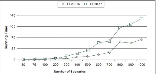
It is worth noting that the path enumeration phase requires a constant amount of time, for all the considered scenario cardinalities. Thus, the exponential behaviour of the running time of AllPEA (see Figure 3.2) is mainly due to the computational effort required to solve the mixed integer problem (17)- (21). As far as the running overhead of SLPA is concerned, the computational results indicate also in this case an exponential trend, but with less variability amongst different reliability levels (see Figure 3.3). In order to assess the influence of the network OS on the running time of the proposed algorithms, we have compared the execution time for the test problems j301 − 1,OS = 0.11 and j3037 − 4,OS = 0.15, both with 30 nodes, for a reliability level of α= 0.8.
Figures 3.4 and 3.5 highlight the related results for AllPEA and SLPA, respectively. From these two figures, it is evident that lower OS levels make the problems more difficult to solve, especially for increasing number of scenarios.
We would like to remark that this trend is more evident for AllPEA. Indeed, a project with a lower order strength has more precedence restrictions
among its activities and therefore, the number of paths to be enumerated is larger.
Figure 3-4: Influence of the order strength on AllPEA running time
Figure 3-5: Influence of the order strength on SLPA running time
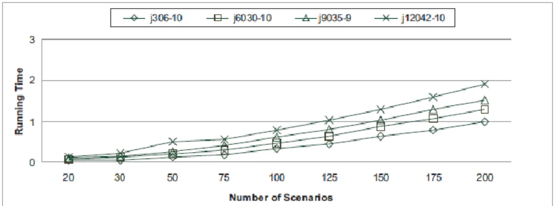
Figure 3-6: Computational time of AllPEA on different test problems
Clearly, the network size (i.e., the number of nodes) plays also a crucial role in the practical efficiency of the proposed solution approaches. In order
to illustrate this aspect, in Figure 3.6 we report the running time of AllPEA, for a probability level of 0.9 and a number of scenarios less than 200, when solving the test problems j306 − 10, j6030 − 10, j901 − 1 and j12042 − 10. The computational results of Figure 3.6 underline that the execution time of the algorithm increases with the number of nodes of the project network, as expected. However, we notice that the time needed to solve all but one of the instances are comparable. This may indicate that a threshold size for the problem to become substantially more difficult is 120 nodes. We would like to remark that even for this instance, the solution time does not exceed 12 seconds. This leaves room for application on even larger instances.
Figure 3-7: Computational time of SLPA on different test problems
Figure 3.7 shows the SLPA computational time for the same test problems. Interestingly, this procedure seems to be less sensitive to the project network dimension. As already observed, a relevant part of the computational time spent by AllPEA is required by the search of all paths of the network, which is exponential in the number of nodes. Finally, we observe that, depending on the project network characteristics, one method may outperform the other. The choice of the most efficient solution approach depends on several factors. To have an idea, let us to consider the two test problems j9047−4 and j909−7. Even though the number of nodes is fixed to 90, and the arcs cardinalities are comparable, the number of paths in the two networks is very different (321 versus 58). Hence, as expected in this case the procedure AllPEA will be computationally more demanding when solving j9047−4. In order to conclude which is the most efficient algorithm, we should compare AllPEA and SLPA over a significant range of complexity measures. Unfortunately, complexity measures are not always useful to explain and predict the time to solve the problem optimally. To support this observation, we remark that the number of paths actually
present in a network drastically affect the solution time. This is evident considering that AllPEA running times for the biggest networks N1 and N2 (with 260 and 380 paths, respectively) are comparable with those of test problems j9047−4 and j9035−9 (with 321 and 381 paths, respectively). Despite these warnings, some conclusions can be drawn on the basis of the numerical results collected. With respect to the comparison between the two solution methods, there is some evidence on the superiority of SLPA over AllPEA at least when the number of scenarios is limited. Indeed, when the number of scenarios is low enough, SLPA outperforms AllPEA; the opposite situation is observed when the scenario cardinality exceeds a certain threshold. This threshold depends on the problem at hand.
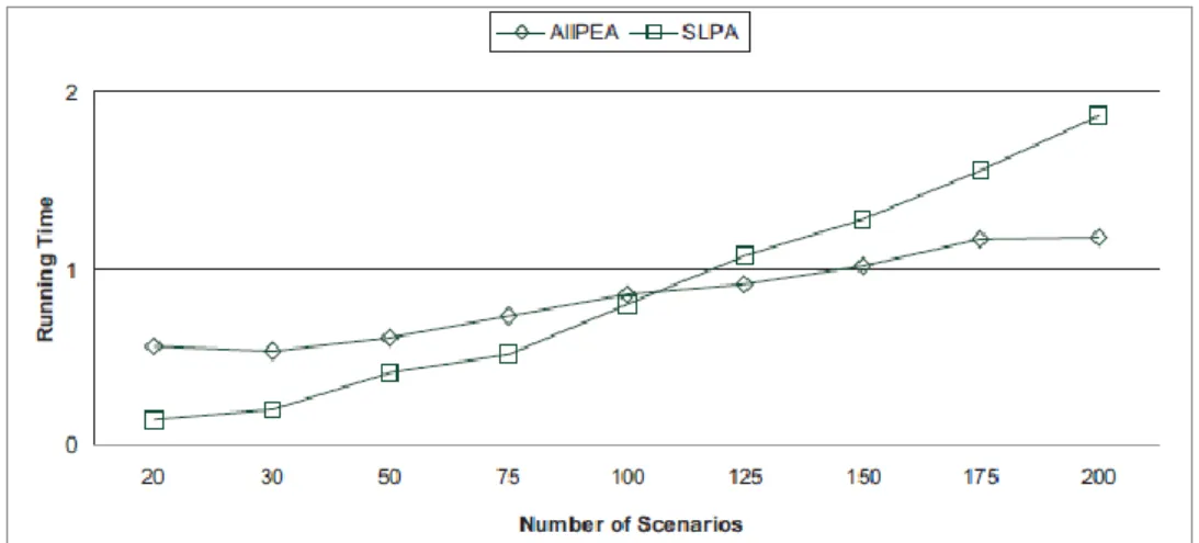
For instance, Figure 3.8 shows the trade-off between the two procedures for the test problem j1201−1 for α = 0.9. We observe that for a scenario cardinality below 100, SLPA is more efficient than AllPEA. When the number of scenarios rises above 100, an opposite behaviour emerges, as AllPEA becomes more efficient than SLPA.
Figure 3-8: Computational time trade-off between AllPEA and SLPA for test problem j1201 − 1
Figure 3.9 is constructed in a similar way as Figure 3.8 for a different test with 60 nodes (i.e., test problem j601−1), but now the threshold scenario cardinality is around 600. Thus, it seems that for smaller networks SLPA performs better notwithstanding the quite high number of scenarios. Nonetheless, it is worth noting that the solution time for the two procedures is quite similar, at least for a scenarios cardinality below the threshold level.
Figure 3-9: Computational time trade-off between AllPEA and SLPA for test problem j601 – 1
Figure 3-10: Computational time trade-off between AllPEA and SLPA for test problem N2, α = 0.99.
We observe that also for the network N2 with a substantially larger number of nodes, the threshold on the number of scenarios is around 650, similarly to the network with 60 nodes (see 3.10). We may regard this indicator as somewhat misleading. However, we should note that this problem instance has a very limited number of paths, which makes the path enumeration phase very efficient in practice. It is worth noting that for some of the instances examined, it is not evident a superiority of one solution method against the other, at least for the number of scenarios considered. For the largest size instances, we report the computational results in Fig. 3.11-3.14. It is worthwhile to remark that these problem instances can be considered quite suitable in order to simulate a real world situation and validate the
behaviour of the proposed model. In fact, a cardinality of 600 for project activities is meaningful related to the typical dimension of a medium term project. Our experiments showed that AllPEA is robust in relation to the number of activities, but, conversely, is highly dependent on the number of paths in the networks. We notice, in fact, that AllPEA running times are higher for the test N1 which has less activities, but more paths than N2. It is worth observing that the computational efforts of the proposed solution methods are not very high, solution times varying over the range [0−400] seconds. Henceforth, the computational results indicate that the procedures are effective even for networks with hundred of activities. On the other hand, the running times drastically increase with the number of scenarios. In this respect, it is worth noting that our model is robust in relation to the number of scenarios used. In fact, in almost all the cases, the makespan found using only 20 scenarios is only a bit different (2% on average) from the makespan evaluated over 1000 scenarios. Nevertheless, we observe that in the case of considering thousand of scenarios, parallel computing could play a crucial role, and this represents the main goal for future development.
Chapter 4
Resource Constrained
Project Scheduling Under
Uncertainty
In this chapter, we study the resource constrained project scheduling problem under uncertainty. Project activities are assumed to have known deterministic renewable resource requirements and uncertain durations, described by random variables with a known probability distribution function. We propose a joint chance constraints programming approach to tackle the problem under study, presenting a heuristic algorithm in which the buffering mechanism is guided by probabilistic information.
4.1. Overview of the problem
The resource constrained project scheduling problem (RCPSP) consists in minimizing the duration of a project, subject to zero-lag finish-start precedence and resource constraints. In its deterministic version, the RCPSP assumes complete information on the resource usage and activities duration, and determines a feasible baseline schedule, i.e. a list of activity starting times, minimizing the makespan value. A solution for this problem is a baseline schedule which specifies, for each activity, the planned starting times. Notwithstanding its importance, the planned baseline schedule may have little, if some value, in real contexts since
project execution may be subject to severe uncertainty and then may undergo several types of disruptions as described in the previous paragraphs. Extensions of the RCPSP, involving the minimization of the expected makespan of a project with stochastic activity durations, have been investigated within the stochastic project scheduling literature. The methodologies for stochastic project scheduling basically view the project scheduling problem as a multi-stage decision process, in which the objective is to minimize the expected project duration subject to zero-lag finish-start precedence and renewable resource constraints. Since the problem is rather involved and an optimal solution is unlikely to be found, scheduling policies (Igelmund & Radermacher (1983), Mohring & Stork (2000), Stork (2000)) and heuristic procedures (Ballestin (2007), Golenko-Ginzburg & Gonik (1998), Golenko-Golenko-Ginzburg & Gonik (1997), Tsai & Gemmil (1998)) have been used for defining which activities to start at random decision points through time, based on the observed past and the a-priori knowledge about the processing time distributions.
Beside this important research area, the field of proactive (robust) project scheduling literature has received outstanding attention in the last years. It entails to incorporate some knowledge of the uncertainty in the decision-making stage, with the aim to generate predictive schedules that are in some sense robust (i.e. insensitive) to future adverse events.
Van De Vonder et al. (2005), (2006) propose the so-called resource flow-dependent float factor heuristic (RFDFF) to obtain a precedence and resource feasible schedule, using information coming from the resource flow network (Artigues et al., 2003) in the calculation of the so called activity dependent float factor (Leus (2003)). In Van de Vonder et al. (2007), several predictive reactive resource constrained project scheduling procedures are evaluated under the composite objective of maximizing both the schedule stability and the timely project completion probability. For an extensive review of research in this field, the reader is referred to Herroelen and Leus (2004b), (2005). Within this research stream, and when abstraction of resource usage is made, we mention the works Herroelen and Leus (2004a), Rabbani et al. (2007), Tavares et al. (1998). When resource availability constraints are considered, Leus and Herroelen (2004), Deblaere et al. (2007) and Lambrechts et al.(2007) and (2008) assuming the availability of a feasible baseline schedule, proposed exact and approximate formulations of the robust resource allocation problem.