Analysis of Reinforced Concrete Elements Including Shear Effects

ACI Structural Journal, V. 103, No. 5, September-October 2006.

MS No. 04-007 received July 25, 2005, and reviewed under Institute publication policies. Copyright © 2006, American Concrete Institute. All rights reserved, including the making of copies unless permission is obtained from the copyright proprietors. Pertinent discussion including author’s closure, if any, will be published in the July-August 2007 ACI

Structural Journal if the discussion is received by March 1, 2007.

ACI STRUCTURAL JOURNAL

TECHNICAL PAPER

This paper deals with the analysis of reinforced concrete (RC) plane frames under monotonic and cyclic loading, including axial, bending, and shear effects. A force-based two-dimensional (2D) element based on the Timoshenko beam theory is introduced. The element formulation is general and yields the exact solution within the Timoshenko beam theory. A simple, nonlinear, shear force-shear deformation law is used at the section level, together with a classical fiber section for the axial and bending effects. Shear deformations are thus uncoupled from axial and bending effects in the section stiffness, but shear and bending forces become coupled at the element level because equilibrium is enforced along the beam element. The element is validated through comparisons with experimental data on the shear performance of bridge columns. The seismic analysis of a viaduct that collapsed during the 1995 Kobe earthquake is presented.

Keywords: beams; reinforced concrete; shear.

INTRODUCTION

Recent years have seen important advances in the analysis of reinforced concrete (RC) frame structures under static and dynamic loads. These advances have originated from the development of new, faster, and more accurate nonlinear frame elements and from the use of refined section models.

Besides classical displacement-based frame elements, force-based elements have been successfully explored. The main motivation for using force-based elements stems from the fact that equilibrium between nodal forces and section forces can be enforced exactly in a beam or column, whereas displacement-based formulations become approximate if the material response is nonlinear. Spacone et al.1 propose a consistent force-based frame element formulation that enforces equilibrium in the strong sense and compatibility in an integral form along the beam element. The main difficulty of force-based elements is their implementation in a general-purpose frame analysis or finite element program, because the nodal forces cannot be computed from the section forces. An iterative procedure is proposed in Spacone et al.1 to solve this problem. The procedure produces the element stiffness and nodal forces corresponding to the nodal deformations. Neuenhofer and Filippou2 propose a simplified version of the original iterative procedure. This simplified procedure basically consists of cutting the iterations to two, relying on the fact that structural convergence will eventually yield element compatibility. The proposed state determination procedures are very robust and work even for elements that exhibit strain-softening, as is the case of RC columns experiencing severe concrete crushing.

Force-based elements are computationally more demanding than displacement-based elements, but they offer the main advantage of being exact within the beam theory framework used for the formulation. This leads to the use of one element

per structural member (beam or column) in a frame analysis, thus requiring a lower number of nodal degrees of freedom. The original force-based formulation by Spacone et al.1 applies to an Euler-Bernoulli beam type,3 which considers only bending and axial deformations. Later model develop-ments have extended the force-based formulations to eledevelop-ments with bond-slip. Salari and Spacone4 discuss the issues related to including slip in steel-concrete composite structures, while Limkatanyu and Spacone5 present the general formulations of line elements with bond-slip. Finally, Sivaselvan and Reinhorn6 extend the nonlinearity of the force-based element to geometric nonlinearities, with a formulation based on a state-space approach.

Another important deformation mode that should be consid-ered in the analysis of RC elements is the shear response. Recent earthquakes have shown that most RC structural failures in older buildings are related to shear deficiencies in the structural elements. Accounting for the shear capacity of beams and columns seems to be the next natural step in the analysis of RC structures with force-based elements. Force-based formulations lead to the exact element flexibility matrix for a linear elastic Timoshenko beam element, that is, an element where the shear deformation is considered constant across the cross section.3 Torsion is uncoupled from axial, bending, and shear deforma-tions in the Timoshenko beam theory.

There are two issues related to shear modeling in force-based elements: the element formulation and the section model. As for the element formulation, Martino et al.7 present the consistent force-based formulation of the Timoshenko beam element with nonlinear material behavior. As for the section model, there can be different approaches to modeling the shear response. One is to extend the original fiber section formulation to account for the shear stresses, deformations, and stiffness. This requires a major reformulation of the concrete constitutive law that must be implemented as biaxial and eventually cyclic for dynamic analyses. Petrangeli et al.8 successfully implemented such a fiber section model, using a concrete law based on the microplane theory. The section, however, demands a consid-erable additional computational cost.

It is important to point out that the shear response of an RC element is more important in terms of strength, than in terms of stiffness. Including the shear stiffness of an RC member does not affect the results of the analyses, as the member stiffness is typically governed by the flexural response. The impact of the shear response becomes apparent when a major Title no. 103-S66

Analysis of Reinforced Concrete Elements Including

Shear Effects

shear crack develops in the frame member, limiting the capacity of the entire member. Following this reasoning, Martino et al.7 decided to use a simplified approach to modeling the shear response of the RC section via a phenomenological

V-γ law. They applied the element to simple pushover analyses

of buildings. The present work generalizes the approach and extends it to cyclic and dynamic analyses.

RESEARCH SIGNIFICANCE

This paper contains the results of research on the modeling aspects of the shear behavior, in particular the shear failure of reinforced concrete structural members. The Timoshenko beam theory is used for modeling shear. The ultimate response of reinforced concrete structures, in particular of existing shear deficient structures designed according to older design codes, is in many cases governed by shear failure. It is important to have simple, though efficient, models that account for the shear strength of reinforced concrete members, particularly when assessing the nonlinear response of reinforced concrete frames under pushover or seismic loads.

REINFORCED CONCRETE ELEMENT WITH SHEAR DEFORMATION Element formulation

The element formulation follows the force-based formulation presented in Spacone et al.1 Bold letters indicate vector and

matrixes, whereas normal letters indicate scalars. Uniaxial bending is considered in this work. The extension to the biaxial case is straightforward. The element is formulated without rigid body modes. The nodal forces, shown in Fig. 1, are the two end moments M₁ and M₂ and the end axial force

N. The corresponding deformations are the two end rotations

θ1 and θ2 and the axial extension u. Element forces and

deformations are grouped in the following arrays

(1)

The section forces are the axial load N(x), the bending moment M(x), and the shear force V(x). The corresponding section deformations are the axial strain at the reference axis ε0(x), the curvature κ(x) and the shear deformation γ(x).

Section forces and deformations are shown in Fig. 2. The resulting strain distributions are also shown. Section forces and deformations are grouped in the following arrays

(2)

Force-based elements stem from the weak (or integral) form of compatibility, expressed through the Principle of Virtual Forces, which in the case of the beam takes the form

(3)

Using equilibrium, the section forces s(x) are written as functions of the end forces P through the force interpolation function N_P(x)

s(x) = N_P(x)P (4)

where

(5)

Finally, the section constitutive law is written

ε(x) = f(x)s(x) (6)

where f (x) is the section flexibility matrix and depends on the section model used for the element.

After substitution of Eq. (4) and (6) in Eq. (3), and after elimination of δPT _{based on the arbitrariness argument,}

the element matrix compatibility equation is written as

P M₁ M₂ N ⎩ ⎭ ⎪ ⎪ ⎨ ⎬ ⎪ ⎪ ⎧ ⎫ = U θ1 θ2 u ⎩ ⎭ ⎪ ⎪ ⎨ ⎬ ⎪ ⎪ ⎧ ⎫ = s x( ) M x( ) N x( ) V x( ) ⎩ ⎭ ⎪ ⎪ ⎨ ⎬ ⎪ ⎪ ⎧ ⎫ = ε x( ) κ x( ) ε0( )x γ x( ) ⎩ ⎭ ⎪ ⎪ ⎨ ⎬ ⎪ ⎪ ⎧ ⎫ = δPT U δsT( )ε xx ( ) xd 0 L

∫

Alessandra Marini is an Assistant Professor in the Civil Engineering Department of

the University of Brescia, Brescia, Italy. She received her MS and PhD from the University of Brescia. Her research interests include the seismic analysis, design, and retrofitting of concrete buildings and of historical heritage.

Enrico Spacone is a Professor in the PRICOS Department, University G.

D’Annunzio of Chieti-Pescara, Italy. He received his BS from the University La Sapienza, Rome, Italy, and his MS and PhD from the University of California at Berkeley, Berkeley, Calif. His research interests include the seismic analysis and the design and retrofitting of concrete buildings and bridges.

Fig. 1—Frame element forces and deformations.

Fig. 2—Timoshenko element: section forces, deformations, and strain distributions.

U = FP (7) where F is the element flexibility matrix without rigid body modes

(8)

The aforementioned equations are formally identical to those of the Euler-Bernoulli beam element, but the element force interpolation functions, the section forces, and the section flexibility are different. The implementation of the aforementioned element in a structural analysis solution scheme follows the lines of the element state determination outlined in Spacone et al.1 and later simplified by Neuenhofer and Filippou.2 In this work, the element is implemented in a general purpose finite element program.9

The nonlinear nature of the element depends entirely on the section nonlinear constitutive law, which is described in detail in the following section.

SECTION CONSTITUTIVE LAWS

There are different ways to formulate the section stiffness and flexibility, depending on the section model that is used. Petrangeli et al.8 extend the fiber section model originally developed for the section of an Euler-Bernoulli beam to the uniaxial bending section model of a Timoshenko beam. The new fiber model necessitates the use of a two-dimensional (2D) law for the concrete and an iterative scheme for each fiber in the cross section. The result is a full 3 x 3 section stiffness matrix that couples axial, bending, and shear responses. Even though the approach by Petrangeli et al.8 is accurate and rational, it is computationally intensive. A simpler approach that follows the original idea discussed in Martino et al.7 is used herein.

At the section level, bending and axial responses are decoupled from the shear response. The layered section is used to obtain the bending and axial responses, which remain coupled. The shear response is modeled via a phenomeno-logical V-γ nonlinear, cyclic constitutive law. The resulting expressions for the section forces S(x) and for the section tangent stiffness matrix k(x) are

(9)

(10)

where n(x) is the number of fibers in the section, σfiber is the

fiber stress, E_fiber is the fiber tangent modulus, A_fiber is the fiber area, and y_fiber is the distance from the fiber centroid to the section reference axis. V = V(γ) indicates that the shear force is computed directly from the shear deformation γ via the selected shear response law, and dV/dγ indicates that the shear tangent stiffness is the derivative of the shear law.

It is worth noting that, while bending and shear forces are not related at the section level, implementation of this constitutive law in a force-based element couples bending and shear forces at the element level through equilibrium. Equation (4) and (5) enforce equilibrium between internal and nodal forces. Therefore, if shear failure at the section level occurs before bending failure, the element bending moments are bound by the element shear forces. This is the main advantage of using a force-based element for a nonlinear Timoshenko beam. Even though the shear and bending responses are not coupled at the constitutive law level, they must be in equilibrium and thus failure in either bending or shear affects the force in either shear or bending. Section shear law

The shear response is modeled using a nonlinear V-γ law. Different envelope curves are shown in Fig. 3. The shear law has an initial parabolic branch and peaks at VRd, γy, which

represents the section shear capacity. A linear branch follows, whose initial and final points are VRd, γy and Vu, γu,

F NP T x ( )f x( )NP( ) xx d 0 L

∫

σfiberAfiberyfiber fiber=1 n x( )

∑

∑

EfiberAfiberyfiber

2

fiber=1

n x( )

∑

n x( )

∑

– 0

EfiberAfiberyfiber fiber=1 n x( )

∑

∑

respectively. The last point represents the residual shear capacity. For γ > γu, V= Vu. By alternatively selecting the

residual shear capacity either smaller or larger than the shear capacity V_Rd, brittle or slightly ductile shear failures can be modeled (Fig. 3, Curves (a) and (a′)). This way, the brittle failure of unreinforced or lightly reinforced concrete beams10 as well as the more ductile failure of fiber-reinforced concrete structures11 or jacket-strengthened members can be modeled.

The definition of V_Rd is a fundamental step in the description of the shear response. According to Park and Paulay12 and to several design codes, the section shear capacity V_Rd is the sum of the steel stirrups contribution VRds at yielding, and

the concrete contribution V_Rdc

VRd = VRdc + VRds (11)

where V_Rdc is

V_Rdc = V_Rdc* +V(N) (12) where V_Rdc* is the contribution of the concrete member under zero axial load, which is mainly a function of the concrete maximum strength and of the amount of longitudinal reinforcement steel, and V(N) is the concrete member capacity enhancement induced by the axial compression

N.12 In the present implementation

(13)

where c is a coefficient that weighs the effect of the axial compression. Eurocode 213 suggests c = 0.15. In the proposed implementation, the shear capacity is updated to take into account the effect of the section axial compression, and the V-γ curve is rescaled at each step (Fig. 3, Curves (a′) and (b′)).

The proposed model also accounts for the damage of the shear strength expected with the progression of the crack pattern.12 As the crack width increases, the stud mechanism as well as the aggregate interlocking resisting effects are jeopardized, thus causing a significant loss of shear capacity. Accordingly, the section shear strength is assumed to decrease linearly

(14) This results in rescaling the shear law, as shown in Curve (c) in Fig. 3.

The damage coefficient C_dam is given by

V N( ) = cN compression V N( ) = 0 tension VRd damaged CdamVRd = (15)

where ε is the tensile strain in the steel farthest from the compression zone. ε1 and ε2 are two limit strain values.

Damage occurs as the shear distortion exceeds the lower limit ε_1, whose value can be set to the yield strain of the longitudinal reinforcing bars (thus ε₁ = ε_y). No further damage occurs when the tensile strain exceeds the limit value ε₂, and the damage coefficient is set to a constant value

C_dam,res.

The hysteretic rules that govern the cyclic response of the shear law are shown in Fig. 4. Upon unloading, a piecewise linear path is followed. The stiffness of the first segment, connecting the two points (Vmax, γmax) and (0, γ0), is set to

the initial stiffness, whereas the stiffness of the second branch leads the response to the point of maximum deformation in the opposite direction, (V_min, γ_min) in the case of Fig. 4. Upon reloading, a similar rule is applied by simply substituting (V_min, γ_min) with (V_max, γ_max).

Eurocode 213 _{largely underestimates the shear capacity V} Rd.

Eurocode 213 poorly accounts for the shear aspect ratio and, therefore, basically neglects the major contribution played by the arch mechanism in resisting the shear forces. The underestimated value of V_Rd leads to conservative shear failure predictions. Other more precise criteria than those previously mentioned can, however, be implemented to estimate the shear capacity V_Rd, depending on the purpose of the analysis.

A first set of analyses showed that the structural response is affected mainly by the shear capacity, whereas it is basically independent of the shear stiffness. Large variations in the value of the shear law initial slope, obtained by imposing different values of γy, produce only negligible changes in the structural

stiffness, which is governed by bending until shear failure (if this occurs).

It is finally important to point out that any section constitutive law exhibiting softening is bound to cause localization and non-uniqueness of the solution. This applies to the section constitutive laws presented in this paper. A thorough discussion of localization issues in force-based elements and a solution of the problem are presented in Coleman and Spacone.14

APPLICATIONS

Cyclic load analysis of University of San Diego Column R3

The proposed Timoshenko beam element was validated by modeling a large-scale reinforced concrete squat column (Column R3) tested by Xiao et al.15 at the University of California, San Diego. The column represents a scaled bridge pier (Fig. 5(a)). In the experimental test, the column top stub and footing were reinforced to avoid premature failure in the joint regions. The column was preloaded with a vertical constant axial load of 114 kips (507.3 kN), then loaded up to failure with a cyclic lateral displacement applied at the column top. The lateral loading system displaced the column in double bending. The early stages were dominated by flexural cracking occurring at the column end regions. The flexural cracks inclined and extended into the web of the columns. With increasing load cycles, the shear cracks penetrated the column mid-height (Fig. 5(b)). The column

ε ε< 1 ε1< <ε ε2 ε ε> 2 Cdam = 1 Cdam 1 ε ε1– ε2–ε1 ---– =

Cdam = Cdam res,

suffered brittle shear failure following the degradation of the truss mechanism induced by yielding of the transverse shear reinforcement (followed by loss of bond). In the experimental tests, shear failure of the column top and bottom ends were prevented by the local shear capacity enhancement induced by the confinement provided by the loading structure.

In the finite element (FE) analyses, the column was modeled by a single force-based frame element, with five Gauss-Lobatto integration points (or monitored sections), whose geometric and mechanical characteristics are listed in Table 1. Experimental and numerical lateral force versus lateral deflection curves are plotted in Fig. 6(a) and (b). Curve A refers to the case without shear failure, which was obtained by assuming a very large shear strength. The case of Curve A is basically equivalent to using a Bernoulli type element. The structure capacity is reached once the ultimate flexural capacity is exceeded in the extreme sections. Curve B was obtained by adopting the shear capacity model suggested by Eurocode 213 (Table 1). By introducing a limited shear capacity, the FE analysis correctly predicts the shear failure of the pier (Fig. 6(b)). The shear capacity is slightly underestimated (Fig. 6(b)). This is due to the limitations of the formula given by Eurocode 2,13 which neglects the increased shear strength due to the arch effect in squat columns.

Shear failure initiation is observed at the column top and bottom regions (Fig. 7(a), Section 5), and propagates toward but never reaches the column mid-height (Fig. 7(b), Section 4). Column mid-height Section 3 behaves similarly to Section 4. The localized shear failure at the column end region is due to the proposed damage model, for which the shear capacity decreases as the section maximum axial strain increases (Eq. (14) and (15)). Given the boundary conditions, the maximum bending moment and, therefore, the maximum axial strain occurs at the supports, thus inducing the highest shear damage at the column ends. The FE shear distortion distribution disagrees with the experimental results, for which shear distortion increases at the column midheight. The different results are due partly to the proposed damage model, and partly to the fact that the numerical analyses cannot take into account the shear capacity enhancement due to the confinement applied to the column ends by the loading structure during the experimental study. While Sections 1 and 5 evolve toward the shear law softening branch and govern the column shear capacity (Fig. 7(a)), Sections 2, 3,

and 4 follow the unloading branches (Fig. 7(b)). It is worth noting that it is damage that induces initiation of the shear failure at the column end sections. If damage was neglected, all sections would behave identically and would fail in shear at the same time (unless round-off errors in the calculations lead to slight differences in the section shear responses). It is worth pointing out that the proposed model allowed the previous analyses to be run in few minutes, while the

Fig. 5—UC San Diego Column R3: (a) vertical and cross sections; and (b) experimental crack pattern at failure.15

Fig. 6—Lateral force versus applied lateral displacement for Column R3: (a) infinite shear strength; and (b) limited shear strength.

Fig. 7—Section shear distortion versus shear force for Column R3: (a) Section 5; and (b) Section 4.

nonlinear FE analysis of the monotonic response of the same column discretized with a 2D mesh lasted for over a week.16 Push-over and dynamic analysis of Hansui Viaduct When the Hyogoken Nanbu earthquake struck Kobe, Japan, in January 1995, a significant number of reinforced concrete structures either collapsed or were severely damaged. The Hansui Viaduct, a single bay, two-level elevated railroad,

collapsed during that earthquake. The Hansui Viaduct static and dynamic responses to seismic actions are analyzed in this section.

Figure 8(a) shows longitudinal and transverse sections of the structure. The height of the frame is 12 m and the overall width of the deck is 11.5 m. The viaduct consists of several identical, independent 30 m long segments. Each segment is supported by two rows of four piers, having 0.9 m square cross sections. Four beams tie together the sets of four piers at their midheight.

The most commonly observed failure mode was either shear or flexure-shear failure of the piers in the transverse direction.17,18 The piers failed just below or above the joint with the midheight beams (Fig. 9(a) and (b)). Figure 9(c) shows the failure sequence proposed by Nishimura,19 which is based on the surveyed damage. Shear cracks developed in the piers close to their joint with the midheight beam. The cracks opened until the spalled concrete fell off and the structure above the cracks slipped sideways.

Because the viaduct consists of a series of identical portal frames in the longitudinal direction, only a single portal frame is studied using the frame element presented in this paper. Both piers and beams were modeled with a single force-based frame element, as shown in Fig. 8(b). It is worth noting that only six elements, with five Gauss-Lobatto integration points each, were necessary to model the entire structure and to run the nonlinear analyses.

A preliminary pushover analysis was performed by applying a monotonically increasing lateral displacement to the deck only. This pushover analysis follows an FE investigation previously performed by Spencer and Shing,20 who used a 2D FE mesh with four-point plane stress elements. Some analyses considered smeared cracks only, whereas others included both smeared and discrete cracks in the concrete. The analyses were quite slow because of the complexity of the material laws and of the refined mesh adopted. The material mechanical properties used in the analyses of this paper are those used by Spencer and Shing20 (Table 2).

Two constant point loads representing the Viaduct self-weight were applied to the top nodes of the two upper piers. Table 1—Geometry and mechanical properties for

FE modeling of UC San Diego Column R3

Cross section A_c = b x h = 16 x 24 in.2 (406 x 610 mm2)

Height 96 in. (2.35 m)

Longitudinal reinforcing bars

22 No. 6 (22φ19.05 mm) uniformly spaced along perimeter; ρ_s = A_s/A_c = 2.5%; concrete cover:

cc = 1.5 in. (37.5 mm)

Steel stirrups 1 No. 2/5 in. (1φ6.35/107 mm); fyw = 47.0 ksi

Concrete f_c = 4.95 ksi; ε_c = 3 × 10–3; ε_cu = 1 × 10–2 Steel fy = 68.1 ksi; εs = 2.3 × 10–3; Es = 29,000 ksi

Shear law

V_Rd = 133 kips*, γ_y = 2.3 × 10–3; V_u† = 22 kips, γ_u = 1.5 × 10–2; c = 0.15 Damage‡: ε1 = 2.3 × 10–3, ε2 = 1.15 × 10–2,

C_{dam, res} = 0.9

*_{By rearranging Eq. (11), (12), and (13), the section shear capacity reads as follows:}

V_Rd = VRdc + VRds = VRdc* + V(N) + VRds

where VRdc* is the concrete shear capacity, as suggested by Eurocode 8: VRdc* =

τrdck(1.2 + 40ρs)bd; τrdc = 0.25fctk,005/γc; fctk,005 = 0.7fctm; fctm = 0.3f2/3 is the mean

value of the tensile resistance; d = h – cc; k = (1.6 – d), where d is expressed in meters; ρs = As/Ac = 2.5%; As is area of anchored tensile reinforcement that extends

(lb + d) beyond the section (lb being anchorage length).

To predict the concrete shear strength, the following assumptions are made: γc = 1;

tensile strength mean value fctm is used instead of fctk,005 in the calculation of τrdc.

This yields to τrdc = 0.25fctm. Therefore, VRdc* ≅ 94 kips. V(N) = cN = 0.15 × 114 ≅ 17 kips.

V_sd = fywAsw0.9d/Δz ≅ 22 kips, where fyw is stirrup yield strength; Asw is the stirrup

cross section area; and Δz is stirrup spacing.

†_V

u = Vsd (residual strength = strength of yielded shear reinforcement).

‡_{To account for shear capacity reduction caused by larger crack openings, the}

assumption is made that damage is triggered by yielding of longitudinal reinforce-ment. Accordingly, the shear law is scaled once maximum axial strain exceeds yield strain of longitudinal reinforcing bars (ε1 = εs). Also, ε2 = 5εs and Cdam,res = 0.9.

Note: 1 ksi = 6.895 MPa; 1 kip = 4.448 kN; and 1 in. = 25.4 mm.

For every structural element, all fiber sections were configured to reproduce the exact position of the reinforcing bars in the concrete cross section. The shear capacity V_Rd* of every integration point was evaluated using the Eurocode 213 formula previously discussed. The changes in the spacing of the steel stirrups along the element axis were taken into account by changing the shear capacity of the relevant integration point. The pushover load-displacement response of the Hansui Viaduct is shown in Fig. 10. Model A assumes infinite shear strength, whereas Model B considers the shear strength of the elements. The Model A response shows a ductile structural response, whereas in the Model B response, the limited shear strength of the piers causes structural failure before the ultimate flexural capacity is reached. The plastic hinge formation history is shown for both analyses in Fig. 11. In the response of Model A in Fig. 10, Point 1a corresponds to the formation of two plastic hinges at the intermediate beam ends (Points 1 and 2 in Fig. 11, Model A). At a higher applied displacement, two plastic hinges developed at the pier supports (Points 3 and 4 in Fig. 11, Model A). The corresponding point in Fig. 10 is Point 2a. Later, the flexural capacity of the upper left pier top is reached (Point 5 in Fig. 11, Model A). This happens for unrealistically high lateral displacements, thus the point is not indicated in Fig. 10.

In the pushover response obtained with Model B, the shear capacity is first reached in the upper left pier (Point 1 in Fig. 11, Model B, Point 1b in Fig. 10). Note that shear failure is reached simultaneously in the upper and lower section of the upper left pier, provided that the steel detailing is identical in the two locations. Simultaneous shear failure of the lower left pier end sections follows (Point 2 in Fig. 11, Model B, Point 2b in Fig. 10). The left piers show early shear failure. The axial tension keeps the left pier shear capacity below that of the right piers, which benefit from the shear capacity enhancement due to axial compression (Eq. (12)). Upon further increase of the lateral displacement, two more plastic

hinges develop, the first one (Point 3 in Fig. 11, Model B, Point 3b in Fig. 10) at the right end of the intermediate beam, and the second one (Plastic Hinge 4 in Fig. 11, Model B, Point 4b in Fig. 10) at the bottom of the bottom right pier. When the last plastic hinge forms, the frame becomes a mechanism. Structural failure is basically reached when shear failure takes place in Column 1 (Point 2b). After Point 2b, as the lateral displacement increases, Columns 1 and 2 soften and Columns 4 and 5 absorb the shear force lost in the left columns. Softening of Column 2 causes a temporary drop in the response between Points 1b and 2b in Fig. 10. Therefore, from Point 2b onward, the curve has a mere numerical meaning.

Spencer and Shing,20 using a model with both discrete and smeared cracks, predicted the shear failure of the Hansui

Fig. 9—Hansui Viaduct: (a) close-up view of pier shear

failures;17,18 (b) most common failures observed along

viaduct; and (c) collapse sequence.19

Table 2—Mechanical properties used in analysis of Hansui Viaduct

Columns Upper beam Midheight beam

Element no. in FE mesh (Fig. 8(b)) 1, 2, 4, 5 3 6 Geometry Cross section 0.9 x 0.9 m 1.1 x 1.1 m 1.1 x 1.1 m Length 6.0 m 5.6 m 5.6 m Longitudinal reinforcing bars 22φ32 mm Top 10φ32 mm Bottom 10φ32 mm Top 2φ32 mm Bottom 6φ32 mm Steel stirrups _{Fig. 8(a))}(refer to φ16/200 mm φ16/175 mm

Material properties

Concrete fc = 26.49 MPa; εc = 0.025%; εcu = 0.5%

Steel f_y = 440 MPa; ε_y = 0.01%; E_s = 210,000 MPa Shear laws

Model A Infinite shear capacity

Model B V_Rd = 0.62 MN γy = 0.115% Vu = 0.63 MN γu = 0.3% V_Rd = 1.34 MN γy = 0.25% Vu = 1.35 MN γu = 0.6% V_Rd = 1.25 MN γy = 0.23% Vu = 1.25 MN γu = 0.6% Model C V_Rd = 0.62 MN γy = 0.115% V_u = 0.30 MN γu = 0.3% V_Rd = 1.34 MN γy = 0.25% V_u = 0.7 MN γu = 0.6% V_Rd = 1.25 MN γy = 0.23% V_u = 0.60 MN γu = 0.6%

Damage ε1 = 0.0023%; εu = 0.023%; and Cdam,res = 0.9

Fig. 10—Pushover response of Hansui Viaduct.

Fig. 11—Failure history in pushover analysis of Hansui Viaduct.

Viaduct for a base shear force of approximately 1.3 kN, corresponding to a lateral deck displacement of 0.066 m. The results obtained with the beam element presented in this paper compare well, in terms of ultimate load, with those obtained by Spencer and Shing20 (Fig. 10). The plane stress model by Spencer and Shing20 is more accurate in predicting a reasonable crack pattern, which cannot be obtained using the beam element proposed herein. On the other hand, the beam element model, requiring six elements only, is less demanding in terms of computational effort, than the 2D model by Spencer and Shing.20 The computational effort prevented them from further investigating the viaduct response under earthquake induced dynamic loads, for which they developed a simplified single degree of freedom system.

Using the mesh of Fig. 8(b), the Hansui Viaduct was then studied under earthquake loads. An input ground motion registered in the Kobe area on January 17, 1995, was applied to the structure. The ground motion has a peak acceleration of 6.7 m/s2 (0.68 g) at time t = 1.66 seconds. The deck mass was obtained from the viaduct original drawings. No live load was assumed to contribute to the mass. Rayleigh damping was used with damping ratios ζ = 3% in the first two modes of vibration.

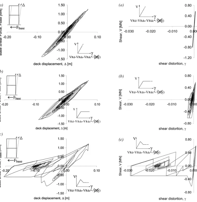
In the first set of analyses, the contribution of the axial compression to the shear capacity was neglected. The bridge dynamic structural response is shown in Fig. 12 in terms of deck displacement versus time. Three different responses, corresponding to different shear models, are shown. Curve a was obtained using a linear elastic shear law with unlimited shear capacity (Model A). Curve b was obtained using an

elastic perfectly plastic shear law (Model B), Curve c used an elastic strain-softening shear response (Model C). The three models remain basically elastic up to t =1.5 seconds. At this time, a plastic hinge forms at the upper beam left end. Afterwards, at time t = 2.2 seconds, the bending capacity is also reached at the beam right end, and another plastic hinge develops. Until t = 2.6 seconds, the response curves are identical, being the nonlinear behavior fully governed by bending (the shear response is still elastic). At time t = 2.6 seconds and time t = 2.7 seconds, shear failures of the lower columns take place in Models B and C (Fig. 13). A peak displacement of –0.08 m is reached at 2.7 seconds (corresponding to a drift of approximately 0.7% the height of the viaduct). At time t = 2.7 seconds, Model A develops a third plastic hinge at the midheight beam left end (Fig. 13).

After t = 4 seconds, the shear capacity in the opposite direction is reached in the right lower columns both in Models B and C. Model C softens; accordingly, Curve c drifts away from the other two curves, which remain very similar as the earthquake action continues. Note that the response in terms of top displacement does not show a major difference between Curves a and b (Fig. 12). After a peak displacement of –0.2 m recorded at time t = 5.3 seconds, a residual displacement of –10 mm is observed for Curve c. Note that the shear failure mode predicted by Model C, accounting for a softening behavior in shear, agrees with the failure mechanism observed on the actual structure (Fig. 9(a)), and with the collapse progress described by Nishimura.19

The Hansui Viaduct response in terms of deck displacement versus lateral force at the base is shown in Fig. 14(a), (b), and (c) for Models A, B, and C, respectively. The analysis of the single section internal force versus deformation curves highlights the formation of a plastic hinge at the upper beam ends (Fig. 13) at time t = 1.5 seconds. Maximum section deformation demand occurs at time t = 5.3 seconds, when all models reach the peak displacements.

Figure 15(a), (b), and (c) show the response in terms of shear force versus shear distortion for the single section of the left lower columns closer to the midheight beam. In Model C, the shear capacity quickly drops to its residual value upon reaching the shear capacity because of the great demand for shear deformation in the following load cycles. The structure collapses at this point and the rest of the response has little physical meaning. The section shear failure occurs for a deck displacement of approximately –0.08 m (Fig. 14(c)) at time t = 2.7 seconds (Fig. 12). Note that the damage, as well as the softening behavior of a few sections along the elements result in a progressive shrinking of the original section shear law, thus causing the irregular shape of the curve plotted in Fig. 14(c).

The second set of analyses accounts for the enhancement of the shear capacity induced by the element axial compression. The behavior of Model A is left unchanged as the increase in shear capacity only affects the shear stiffness. The structural response in terms of time versus deck displacement remains basically the same for both Models A and B (Fig. 16, Curves (a) and (b)), whereas a noteworthy reduction of the maximum deck displacement is recorded in Model C (Fig. 16, Curve (c)). Plastic hinges in the upper beams still form at time t = 1.5 seconds in all models, but the enhanced shear capacity delays the left lower column shear failure in Models B and C until time t = 5.29 seconds, corresponding to a deck displacement of –86.2 mm. In Model C, the peak displace-ment is reduced to –0.1 m at time t = 6.7 seconds, and the

Fig. 12—Hansui Viaduct dynamic response to Kobe earth-quake for different V-γ curves, obtained neglecting influence of axial compression on section shear capacity.

Fig. 13—Failure modes for different V-γ curves, obtained

neglecting influence of axial compression section shear capacity.

deck residual drift drops to –0.03 m, compared with the cases with no increase in shear capacity.

The structural response in terms of base shear versus deck displacement is shown in Fig. 17 for Models B and C. With the axial compression contribution, the shear capacity enhancement is approximately equal to 20%.

Figure 18 shows the failure mode for the three models. The axial compression does not modify the plastic hinge distribution of Model A, nor the collapse mechanism for Model C. Conversely, Model B develops shear failure in the left lower and right upper columns, preventing the formation of a mechanism and thus avoiding structural collapse. The failure mode predicted for Model C agrees with the failure mode of the actual structure (Fig. 9(a)).

Figure 19(a) and (b) show the single section response for Models B and C obtained by alternatively considering or neglecting the term V(N) in Eq. (11) and (12). The section shear capacity enhancement is approximately equal to 20%. When accounting for the V(N) term, the maximum section

Fig. 14—Base shear force versus deck displacement for

different V-γ curves, obtained neglecting the influence of

axial compression on section shear capacity.

Fig. 15—Section shear force versus shear distortion for

different V-γ curves, obtained neglecting the influence of

axial compression on section shear capacity.

Fig. 16—Hansui Viaduct dynamic response to Kobe

earth-quake for different V-γ curves, obtained accounting for the

shear distortion of Model C is significantly reduced, and the deck drift decreases accordingly.

The aforementioned results show that accounting for the increase in shear capacity due to axial compression leads to qualitatively reasonable results in terms of failure mechanism and displacements. Only the few elements undergoing compression benefit from the shear capacity increase. Plastic hinges and shear failures develop at the weak points in the structure. Furthermore, the adoption of a softening branch following the peak shear point results in large residual displacements. Conversely, assuming a perfectly plastic behavior in shear still allows triggering the shear failure of the structure, but produces unrealistically small deck drifts throughout the analyses.

CONCLUSIONS

A force-based element based on the Timoshenko beam theory is presented in this paper. The element formulation

can be regarded as general and is exact within the Timoshenko beam theory. A phenomenological shear force-shear deformation law is used at the section level, together with a fiber section model for the axial and bending effects. Shear and bending are decoupled in the section constitutive law, but equilibrium between them is enforced, thus bending and shear are coupled at the element level. The proposed shear constitutive law accounts for the increase in shear capacity due to axial compression, as well as for the damage caused by excessive crack opening. The element is implemented in a general purpose FE program, and validated by means of FE analyses of RC columns and frames subjected to cyclic push-over and earthquake loads.

The results of a first set of correlation studies with the experimental results on a bridge pier show that the model is able to capture the shear failure of the squat column and provides qualitatively reasonable results both in terms of maximum lateral base force and column top displacement. The shear capacity of the pier was slightly underestimated, due to the conservative evaluation of the pier shear capacity based on Eurocode 2,13 which poorly accounts for the arch mechanism contribution that becomes more important in shorter members.

A second set of analyses focuses on modeling the response of the Hansui Viaduct under both pushover and earthquake loads. The results highlight the importance of accounting for the limited shear capacity of the piers in predicting the failure mechanism of the structure. The results of the push-over analysis are in good agreement with a previous nonlinear FE analysis of the viaduct. Softening or perfectly plastic branches of the shear law can be alternatively selected to describe the behavior of ordinary or high performance concrete structures. When softening is selected, the energy

Fig. 17—Base shear force versus deck displacement for different V-γ curves, obtained accounting for the effect of axial compression on section shear capacity.

Fig. 18—Failure modes for different V-γ curves, obtained

accounting for the effect of axial compression on section shear capacity.

Fig. 19—Section shear force versus distortion for different

V-γ curves, obtained accounting for the effect of axial

dissipation capacity of the structure changes considerably and the results show large residual displacements at the end of the seismic event. Besides, the predicted shear failure mechanism agrees with the failure mode of the real structure. On the other hand, assuming a perfectly plastic behavior in shear produces unrealistically small deck drifts throughout the analyses.

Future studies will concentrate on the selection of more accurate formulas for the prediction of the shear capacity of beams and columns. In particular, such laws should account for the effects of the shear span ratio on the shear capacity. Another extension of the element formulation should explore the development of a fiber law that also accounts for the shear deformations. It is, however, worth underlining that the proposed element allows accounting for the shear failure of RC members in a simple and computationally efficient way. Considering the shear deformations at the fiber level would incorporate other phenomena, such as aggregate interlock and possibly dowel actions, but it would make the element computationally very expensive, and thus slow.

ACKNOWLEDGMENTS

This study was partially supported by Grant CMS-9804613 from the National Science Foundation. This support is gratefully acknowledged. Any opinions expressed in this paper are those of the authors and do not reflect the views of the sponsoring agencies. Special thanks go to F. Seible for providing the authors with all data of the cyclic tests on reinforced concrete columns performed at the University of California, San Diego, San Diego, Calif.

NOTATION

A_fiber, E_fiber, y_fiber= fiber area, modulus and distance from reference axis, respectively

Cdam = damage coefficient

D = element nodal deformation array

F, f = element and section flexibility matrixes

k = section stiffness matrixes, respectively M1, M2, N = element nodal forces

M(x), N(x), V(x) = section forces

N_P(x) = force interpolation functions

P = element nodal force array

s(x), ε(x) = section force and deformation arrays, respectively V(N ) = shear capacity provided by element axial

com-pression

V_Rd, γ_y = maximum shear capacity and shear distortion, respectively

= damaged shear capacity

V_Rdc,V_Rdc* = shear capacity provided by concrete by either considering or neglecting axial load contribution, respectively VRds = shear capacity provided by steel stirrups

V_u, γ_u = residual shear capacity and shear distortion, respectively

κ(x), ε(x), γ(x) = section deformations θ1, θ2, u = element nodal deformations

σfiber = fiber stress

REFERENCES

1. Spacone, E.; Filippou, F. C.; and Taucer, F. F., “Fiber Beam-Column Model for Nonlinear Analysis of R/C Frames, Part I: Formulation,” Earth-quake Engineering and Structural Dynamics, V. 25, 1996, pp. 711-725.

2. Neuenhofer, A., and Filippou, F. C., “Evaluation of Nonlinear Frame Finite-Element Models,” Journal of Structural Engineering, ASCE, V. 123, No. 7, 1997, pp. 958-966.

3. Timoshenko, S. P., and Goodier, J. N., 1970, Theory of Elasticity, 3rd Edition, McGraw-Hill, Inc., New York.

4. Salari, M. R., and Spacone, E., 2001, “Analysis of Steel-Concrete Composite Frames with Bond-Slip,” Journal of Structural Engineering, ASCE, V. 127, No. 11, pp. 1243-1250.

5. Limkatanyu, S., and Spacone, E., 2002, “R/C Frame Element with Bond Interfaces, Part 1: Displacement-Based, Force-Based and Mixed Formulations; Part 2: State Determination and Numerical Validations,” Journal of Structural Engineering, ASCE, V. 128, No. 3, pp. 346-364.

6. Sivaselvan, M. V., and Reinhorn, A. M., 2002, “Collapse Analysis: Large Inelastic Deformations Analysis of Planar Frames,” Journal of Structural Engineering, ASCE, V. 128, No. 12, pp. 1575-1583.

7. Martino, R.; Spacone, E.; and Kingsley, G., 2000, “Nonlinear Pushover Analysis of R/C Structures,” Structures Congress, Advanced Technology in Structural Engineering, M. Elgaaly, ed., ASCE, 8 pp. (CD-ROM)

8. Petrangeli, M.; Pinto, P. E.; and Ciampi, V., 1999, “Fiber Element for Cyclic Bending and Shear of R/C Structures, Part I: Theory,” Journal of Engineering Mechanics, ASCE, V. 125, No. 9, pp. 994-1001.

9. Taylor, R. L., 2000, “FEAP: A Finite Element Analysis Program,” User Manual, Version 7.3., Department of Civil and Environmental Engineering, University of California at Berkeley, Berkeley, Calif., http://www.ce.berkeley.edu/~rlt/feap/.

10. Giuriani, E.; Adami, P.; Minelli, F.; and Pozzani, G., 2003, “Resistenza a taglio nelle travi in c.a.,” Internal Report, Universit degli Studi di Brescia, Dipartimento di ingegneria civile. (in Italian)

11. Meda, A.; Minelli, F.; Polizzari, G. A.; and Failla, C., 2002, “Experimental Study on Shear Behavior of Prestressed SFR/C Beams,” 6th International Symposium on Utilization of High Strength/High Performance Concrete, Lipsia, Germany, June.

12. Park, R., and Paulay, T., 1975, Reinforced Concrete Structures, John Wiley & Sons, Inc., 1975, 800 pp.

13. Eurocode No. 2, 1991, “Design of Concrete Structures—Part 1-1: General Rules and Rules for Buildings,” ENV 1992-1-1, Brussels.

14. Coleman, J., and Spacone, E., 2001, “Localization Issues in Nonlinear Force-Based Frame Elements,” Journal of Structural Engineering, ASCE, V. 127, No. 11, pp. 1257-1265.

15. Xiao, Y.; Priestley, N.; and Seible, F., 1993, “Steel Jacket Retrofit for Enhancing Shear Strength of Short Rectangular Reinforced Concrete Columns,” Report No. SSRP-92/07, Structural Systems Research Project, University of California-San Diego, San Diego, Calif.

16. Kang, H. D.; Willam, K.; Shing, B.; and Spacone, E., 2000, “Failure Analysis of R/C Columns Using a Triaxial Concrete Model,” Computers and Structures, V. 77, No. 5, pp. 423-440.

17. De Marco, R.; Decanini, L.; Sanò, T.; and Orsini, G., 1995, “Il Terremoto di Kobe del 17 Gennaio 1995—Rapporto,” Istituto Poligrafico e Zecca dello Stato, Roma. (in Italian)

18. Kitagawa, Y., and Hiraishi, H., 2004, “Overview of the 1995 Hyogo-Ken Nanbu Earthquake and Proposals for Earthquake Mitigation Measures,” Journal of Japan Association for Earthquake Engineering, V. 4, No. 3, pp. 1-29.

19. Nishimura, A., 2004, “Damage Analysis and Seismic Design of Rail-way Structures for Hyogoken-Nanbu (Kobe) Earthquake,” Journal of Japan Association for Earthquake Engineering, V. 4, No. 3, pp. 184-194.

20. Spencer, B., and Shing, P. B., 2001, “Earthquake Damage to the Hansui Viaduct: A Case Study,” personal communication, University of Colorado at Boulder, Boulder, Colo.

VRd damaged