3-D Field Intensity Shaping via
Optimized Multi-Target Time Reversal
Gennaro G. Bellizzi Student Member, IEEE, Martina T. Bevacqua,
Lorenzo Crocco Senior Member, IEEE and Tommaso Isernia Senior Member, IEEE
Abstract—Generating given 3-D field intensity distributions in a non homogeneous scenario is a canonical problem which is of interest in many applications. On the other side, due to its very challenging nature, very few methods have been proposed up to now in the literature for its solution. In this work, starting from the well-known time reversal technique, a simple innovative approach, the so-called optimized multi-target time reversal, is presented. The strategy has been tested in a 3-D in-homogeneous scenario and compared to a previous time-reversal-based shaping technique, named multi-target time reversal. Results show that the proposed approach outperforms the benchmark approach in terms of coverage of the target areas, and it is able to achieve the desired field intensity distribution in a number of cases where the existing benchmark approach completely fails.
Index Terms—Antenna array; Multi-spot focusing; Phase shift; Spatial field shaping; Time reversal.
I. INTRODUCTION
Controlling the field intensity within an in-homogeneous medium is both an interesting problem from a theoretical point of view as well as an essential and decisive step for many practical applications. In different contexts, indeed, spanning from the medical one [1], [2] to near field focusing [3]–[5], the possibility of shaping the field intensity over an extended target area or focusing it in two (or more) target regions, represents a pivotal need. Such a tight control of the field intensity, however, cannot be achieved by means of the different approaches already present in the literature which are “only” able to focus a wave-field in a target point, e.g., focusing via constrained power optimization (FOCO) [6], time reversal (TR) [7], [8], inverse filter [9], to name a few. Hence, the paradigm of focusing a wave-field in a target point needs to be modified in order to deal both with extended and multi-spot target areas.
Probably because of the intrinsic challenging nature of the problem, only a few approaches able to address this need can be found in the literature (which are briefly reviewed in the following). In all of them (and in the remainder of this paper), the problem is generally tackled by properly designing the complex excitations of an array of fixed geometry. By the sake of simplicity, we will refer throughout to the case of scalar fields (deferring some limits on the vector case
to the Conclusions). This is the case of ultrasound field in biological tissues or the case of electromagnetic fields when one component can be considered dominant above the other ones. Also note we deal herein with monochromatic fields.
A very simple shaping strategy, proposed in [10], amounts to add the contributes gathered by solving, through TR, several focusing problems into different target points, named “control points”, placed within a certain target area. Being based on TR, this shaping procedure, named multi-target TR (mt-TR), allows to control to some extent the field intensity through a proper choice of the distance among the control points. However, it cannot enforce any constraints on the power deposition outside the target area. On the other hand, mt-TR requires a very low computational burden and it is easily implementable. In fact, it just requires to solve a number of forward problems by locating a unit-excited point source in correspondence of the control points. The fields radiated at the antennas locations are recorded, and the complex conjugate of these fields become the excitations of each (single target) focusing problem. Finally, the excitations corresponding to the different (single target) focusing problems are simply added.
Another shaping procedure, the so-called multi-target FOCO, has been very recently proposed and tested in [11]. This technique, cast as the solution of a number of convex programming problem, is able to gather the desired field intensity distribution and at the same time enforce given upper bounds constraints outside. Even if the globally optimal solution can be determined1by means of off-the-shelfs search
algorithms, this procedure has a non trivial computational burden.
Motivated by the lack in the literature of methods such to be both computationally and practically efficient, we propose in the following an innovative shaping procedure. In particular, starting from the above mentioned mt-TR and noticing that this corresponds to exploit in-phase focused fields in the different control points, the developed procedure proposes a more effective (still very simple) strategy, based on the same basic bricks, which allows to improve performances in
1Under certain requirements and conditions - details in [11], [12].
This is the pre-peer reviewed version of the following article: Gennaro G. Bellizzi, Martina T. Bevacqua, Lorenzo Crocco, Tommaso Isernia, “3-D Field Intensity Shaping via Optimized Multi-Target Time Reversal”, IEEE Trans. on Antennas and Propagation, vol. 66, is. 8, pp. 4380-4385, 2018. Article has been published in final form at: https://ieeexplore.ieee.org/document/8368155/?arnumber=8368155source=authoralert/
1536-1225 2009 IEEE Personal use of this material is permitted. Permission from IEEE must be obtained for all other uses, in any current or future media, including reprinting/republishing this material for advertising or promotional purposes, creating new collective works, for resale or redistribution to servers or lists, or reuse of any copyrighted component of this work in other works.
This is the postprint version of the following article: Gennaro G. Bellizzi, Martina T. Bevacqua, Lorenzo Crocco, Tommaso Isernia, “3-D Field Intensity Shaping via Optimized Multi-Target Time Reversal”, IEEE Trans. on Antennas and Propagation, vol. 66, is. 8, pp. 4380-4385, 2018. Article has been published in final form at: https://ieeexplore.ieee.org/document/8368155.
terms field intensity shaping. The basic idea of the proposed technique, named optimized multi-target TR (O-mt-TR), is that one can combine the bricks of the above described mt-TR procedure (i.e., fields and excitations of the single target problems) in a different fashion. In particular, the proposed procedure simply explores different phase shifts among the excitations of the single target problems. Then, observation of the performances achieved by the different superpositions will allow to a-posteriori determine the one leading to some “optimal” field intensity distribution.
Besides presenting the proposed O-mt-TR, we also provide a numerical assessment with a twofold aim. In fact, the analysis will allow to evaluate the actual improvements with respect to the benchmark mt-TR. Moreover, one can get a preliminary and empirical understanding of the more appropriate choice of the control points in order to shape (uniformly within a certain area either in a multi-spot focused configuration) the field intensity within a 3-D in-homogeneous scenario.
The remainder of the paper is organized as follows. In Sect. II, after a brief recall of the mt-TR, the formulation of the proposed approach is given. The description of the setup and of the different scenarios considered in the numerical analysis are reported in Sect. III, whereas results analysis and their discussion are in Sect. IV. Finally, conclusions and final remarks follow in Sect. V.
II. THEPROPOSEDAPPROACH
A. Multi-Target Time Reversal
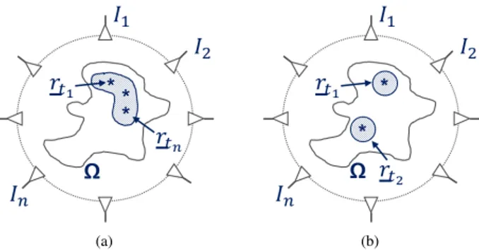
Let ⌦ be a generic 3-D region of interest surrounded by N elementary monochromatic electric sources as shown in Fig.1. Indicating with n(r) the total scalar field induced by the
unitary excited n-th antenna in ⌦ when all the other antennas are off, the overall field in a generic point of r 2 ⌦ can be expressed as: E(r) = N ’ n=1 In n(r) (1)
where In(n = 1, 2, ..., N) is the set of complex excitation
coefficients.
As in other shaping approaches [10], [11], let us consider a set of control points, say rt i (i = 1, .., L), arbitrary located
into the target area. For sake of visualization, Fig.1.(a) depicts the case of an extended target area whereas Fig.1.(b) depict the case of a multi-spot (dual-spot) target areas.
Denoting with n(rt i) the total field measured by the n-th
antenna when a unit amplitude point source is located into
(a) (b)
Fig. 1. Sketch of the scenario used by O-mt-TR in case of extended or multi-spot target area (a and b, respectively). The target area, enlighten by a darker background, contains the control points indicated by the big blue stars.
the control point rt i, according to the standard TR theory, the
focused field in rt iwould be provided by: Ei(r) = N ’ n=1 ⇤ n(rt i) n(r) (2)
where ⇤ denotes the conjugation operation.
A first “basic” shaping approach is the so-called mt-TR [10] and it is cast as a simple sum of the excitations corresponding to different control points, so that:
E(r) = N ’ n=1 L ’ i=1 ⇤ n(rt i) n(r) (3)
which simply corresponds to sum the excitations related to the different focusing problem.
B. Optimized Multi-Target Time Reversal
By the sake of simplicity, let us refer to the case of just two control points and let 2 [0, 2⇡] be an auxiliary variable indicating the phase shift between the fields in rt1 and rt2 (as computed from single target TR).
As such, the O-mt-TR approach, for each (sampled) value of , casts the shaping problem as the combination through complex unit amplitude coefficients, of the fields focused in correspondence of rt1 and rt2 through TR. The excitations
coefficients could be determined as:
In= n⇤(rt1) + n⇤(rt2)ej (4)
where is another degree of freedom of the problem. The optimal solution can be efficiently determined by observing a-posteriori the results achieved at the different values, and picking the most convenient one according with the application at hand.
One possibility consists in selecting amongst the different solutions the one providing the best trade off between the field intensity distribution closest to the desired one within the target area and the lowest side peak elsewhere. Alternatively, a simpler possibility, which is the one adopted in the following, consists in selecting the optimal as the one maximizing the sum of the squared amplitude of the field in the control points, i.e., ÕL
i=1E(rt i) 2
.
The generalization to the case of L control points and M sampled values of the auxiliary variables will require ML 1
linear superposition, thus impacting the computational burden. On the other side, differently from [11], one just has to compute linear superposition (rather than solving the same number of CP problems). Also, one can take profit from parallel computing.
III. EVALUATIONSETUP ANDRATIO
The 3-D scenario used for the validation is depicted in Fig. 2.(a) and consists in two dielectric objects (a cube and a sphere) contained by a spherical region of interest, i.e. ⌦, which is hosted in free space. The spherical region of interest has a diameter of d⌦ = 2, 5 bg2 and a relative permittivity
equal to ✏⌦=2, the cube has a side of lc= bg/2 and ✏c=2,
whereas the sphere has a diameter of ds= bg/4 and ✏s=3.
The antennas array is cylindrical array of radius r ⇡ 2 bg
made up by 65 very small unitary-excited dipoles, arranged over 5 equi-spaced circles, along the z-axis (i.e., 13 per circle), as shown in Fig. 2.(b). Numerical simulations have been performed with a 3-D full wave finite element solver with a working frequency of 1, 5GHz. Finally, only the z-component of the field has been optimized since, according to the antennas configuration, this component can be considered to be dominant above the others.
The following numerical analysis is articulated in three different parts.
2Being
b g the wavelength in the background medium
(a) (b)
Fig. 2. Scenario used for validation (a) and antenna array configuration (b).
(a) (b)
(c)
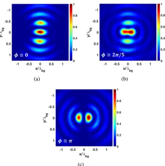
Fig. 3. Three solutions obtained by means of the O-mt-TR with control points set at ⇡ 0.4 b g.
First, the relevance of the phase shift is discussed and emphasized. To this end, two control points have been placed along the x-axis at a distance of approximately 0.4 bg. Then,
excitations (4) have been used with different values, and the different solutions observed. In this starting example, as well as in the numerical experiments described in the fol-lowing, 20 values of have been uniformly sampled between 0 and 2⇡.
Second, we have tested the capability of the proposed approach to achieve a (nearly) uniform shaping of the field intensity over an extended target area. To this end, an extended ellipsoidal shaped target volume, of axes ⇡ 3 bg/2 ⇥ bg/3 ⇥ bg/3, has been placed in two different positions3 in ⌦
(configurationsI and II in the following). In order to get the desired shaping, three control points have been used and have been arranged uniformly (with a spacing of ⇡ 0.4 bg) along a
segment centered on the center of mass of the target volume. In order to better appreciate the differences with respect to mt-TR, the coverage factor (indicated by CF and defined as the fraction of the target area in which E(r)2 is higher than 50% of its maximum value4 [13]) has also been reported and
discussed.
Third, we prove the capability of the proposed approach to get a multi-spot behavior of the field intensity even in case of sub-wavelength spots spacing (which is unfeasible with mt-TR). To this end, two control points have been placed at a
3With the main dimension oriented along the z-axis. 4Ideally CF=1.
distance varying from ⇡ 0.4 bgto ⇡ 2 bgalong the x- and the
y-axes. Then, the O-mt-TR and the mt-TR have been applied and compared. Moreover, in order to validate the approach for an even more difficult case, two different configurations (sayA andB) with three control points have been considered. In these latter examples the control points have been set at a distance approximately equal to 0.65 bg and 0.4 bg from the central
point along the x- and y-axes, respectively. Concerning this third analysis, dealing with the “multi-spots” field intensity shaping, the target volume has been modeled as spheres of diameters ⇡ bg/3 centered in the control points5 [14]–[16].
Note that also in this last analysis, the CF has been adopted in order to estimate the performances of the two TR-based approaches.
IV. RESULTS: ANALYSIS& DISCUSSION
As a first result helping to understand the role of the
auxiliary parameter , Fig. 3 depicts three solutions,
related to the first numerical experiment described in the previous Section. As it can be seen, different choices of the additional parameter allow to pass from a kind of shaped intensity (see Fig. 3.(b)) to a dual-spot configuration (see Fig. 3.(c)). In the same graph, Fig. 3.(a) represents the mt-TR.
5These analyses were not conducted along the z-axis as the cylindrical array
configuration, while being realistic, does not allow a tight control of the field in this dimension.
(a) (b)
(c) (d)
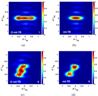
Fig. 4. Squared amplitude of the field, for the configurationsI and II, obtained by means of mt-TR and O-mt-TR in a cut view along the of the target area. Target area is as black line.
Fig. 5. Coverage factor obtained by means of mt-TR and O-mt-TR with respect to control points distance for two control points along the x and the y axes respectively depicted in green (circle and stars) and blue (rhombus and squares).
(a) (b)
Fig. 6. Squared amplitude of the field for dual-spot focusing with control points distance ⇡ 0.5 b g, obtained by means of O-mt-TR and mt-TR. Target
area is in black plain line.
As far as the possibility to achieve uniformly shaped field intensities is concerned, Fig. 4 depicts the normalized squared amplitude of the fields obtained by means of O-mt-TR for both configurations I and II. In addition to what can be visually appreciated, from a quantitative point of view, O-mt-TR is able to significantly enhance the uniformity of the field intensity within the target region with respect to mt-TR. In fact, for configuration I, the CF increases from 44% to 71%, whereas for configuration II it raises from 39% to 81%. Note that the proposed approach not only outperforms the standard mt-TR in terms of CF, but in some cases, e.g., configuration II, is able to gather an uniform coverage of the target area which cannot be achieved at all by means of mt-TR (see Fig. 4.(b)-(d)).
As far as the multi-spot case is concerned, Fig. 5 depicts the CFs related to both O-mt-TR and mt-TR for the two dual-spot focusing configuration (i.e., along the x- and y-axes) as a function of the control points distance. From this plot, two different kind of results can be identified depending
on whether the spacing is below or besides a threshold of approximately 0, 8 bg. While for more “distant” control points
an average improvement on CF of ⇡ 10% can be achieved, when the control points distance is smaller than ⇡ 0.8 bg,
O-mt-TR outperforms the mt-TR on average by 20% (and up to ⇡ 45%). Similarly to the previous analysis, O-mt-TR is not only able to improve mt-TR performances, but it is also delivers a dual-spot focused field intensity distribution where the un-optimized approach fails, as shown in Fig. 6. More in detail, Fig. 6 depicts a cut view along the target areas of the normalized squared amplitude of the field obtained by means of mt-TR and O-mt-TR when target points are distant ⇡ 0.5 bg.
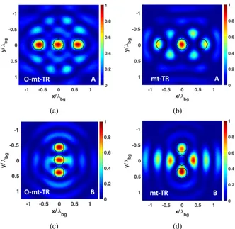
Similar reasonings and performances can be observed in the three spots cases. In these cases, indeed, as shown in Fig. 7, the CF is increased from 35% to 79% for configuration A and similarly from 38% to 77% for configuration B. Apart from the metrics, which confirm the remarkable improvement, it is worth to note that in case of multi-spot focusing the O-mt-TR comes to be fundamental as the standard approach completely fails - see Fig. 7.(b)-(d).
From these results we can conclude that the auxiliary parameters represented by the phase shifts between the field in the different control points, plays a role which is more and more relevant as the control point distance became smaller. As a matter of fact, when dealing with “distant” control points and multi-spot requirements, the additional degrees of freedom, while still relevant, are not necessary to avoid the failure of the field intensity control. Conversely, controlling the phase shifts becomes essential to deliver either a uniformly shaped or sub-wavelenght multi-spot focused field intensity distribution. Let us finally note that the approach can be eventually extended to the case of a non-uniform shaping by inserting a given amplitude factor in the last term of eq. (4).
V. CONCLUSIONS
In this work we have presented an innovative and relatively simple method to spatially shape the intensity of a (scalar) field. The usefulness and the performances of the technique have been shown in cases where uniform shaping or multi-spot configurations are required.
The proposed approach, originated as an optimized version of the existing mt-TR, relies on the use of a set of properly located control points. Then, by exploiting the additional degrees of freedom of the problem, represented by the phase shifts of the field in the different control points, the O-mt-TR is able to optimize the coverage within the target area at a relatively low computational burden.
The approach has been tested in 3-D in-homogeneous scenario and compared to the existing mt-TR. Results, which
(a) (b)
(c) (d)
Fig. 7. Squared amplitude of the field for multi-spot focusing with control points at ⇡ 0.65 b gand ⇡ 0.4 b g((a)-(b) and (c)-(d), respectively), obtained
by means of O-mt-TR and mt-TR. Target area is in black plain line.
are representative of a more extensive analysis, confirm that O-mt-TR outperforms the benchmark mt-TR.
Applicability of the technique is presently limited to the case of a moderate number of control points. Hence, efforts are currently devoted to find more effective procedures to extract the optimal values of the phase shifts, including a-priori exclusion of a subset of values, local optimizations, as well as recurrent rules on the “optimal” values. This will consequently allow to keep curbed the computational burden of the procedure when dealing with vector fields (which can be developed by taking into account [17]). Finally, future plans are also aimed at testing the O-mt-TR as a planning tool in hyperthermia treatment [18], [19].
REFERENCES
[1] P. Wust, B. Hildebrandt, G. Sreenivasa, B. Rau, J. Gellermann, H. Riess, R. Felix, and P. Schlag, “Hyperthermia in combined treatment of cancer,” The Lancet Oncology, vol. 3, no. 8, pp. 487–497, 2002.
[2] M. M. Paulides, G. M. Verduijn, and N. V. Holthe, “Status quo and directions in deep head and neck hyperthermia,” Radiation Oncology (2016) 11:21, 2016, DOI 10.1186/s13014-016-0588-8.
[3] M. Merenda, I. Farris, C. Felini, L. Militano, S. C. Spinella, F. G. D. Corte, and A. Iera, “Performance Assessment of an Enhanced RFID Sensor Tag for Long-run Sensing Applications,” IEEE SENSORS, 2014. [4] M. Merenda, F. D. Corte, and M. Lolli, “Remotely powered smart RFID tag for food chain monitoring,” Sensors and Microsystems, pp. 421–424, 2011.
[5] C. Hsi-Tseng, H. Tso-Ming, W. Nan-Nan, C. Hsi-Hsir, T. Chia, and P. Nepa, “Design of a near-field focused reflectarray antenna for 2.4 GHz RFID reader applications,” IEEE Trans. Ant. Prop., vol. 59, no. 3, pp. 1013–1018, 2011.
[6] D. A. M. Iero, T. Isernia, A. F. Morabito, I. Catapano, and L. Crocco, “Optimal Constrained Field Focusing for Hyperthermia Cancer Therapy: a feasibility assessment on realistic phantoms,” PIER, pp. 125–141, 2010.
[7] M. Fink, “Time reversal of ultrasonic fields. i. basic principles,” IEEE Trans. Ultrason. Ferroelectr. Freq. Control., vol. 39, pp. 555–566, 1992. [8] P. Takook, H. D. Trefna, X. Zeng, A. Fhager, and M. Persson, “A Computational Study Using Time Reversal Focusing for Hyperthermia Treatment Planning,” Progress In Electromagnetics Research B, vol. 73, pp. 117–130, 2017.
[9] E. Zastrow, S. Hagness, and B. VanVeen, “3D computational study of non-invasive patient-specific microwave hyperthermia treatment of breast cancer,” Phys. Med. Biol., vol. 55, pp. 3611–3629, 2010. [10] D. Zhao and M. Zhu, “Generating Microwave Spatial Fields with
Arbitrary Patterns,” IEEE Antennas and Wireless Propagation Letters, no. 99, pp. 1–4, 2016.
[11] G. G. Bellizzi, D. A. M. Iero, L. Crocco, and T. Isernia, “Towards 3D Intensity Shaping:The Scalar Case,” IEEE Antennas and Wireless Propagation Letter, 2017.
[12] G. G. Bellizzi, L. Crocco, D. A. M. Iero, and T. Isernia, “Arbitrary field intensity shaping via multi-target optimal constrained power focusing,” Antenna Technology: Small Antennas, Innovative Structures, and Appli-cations (iWAT), 2017 International Workshop on, pp. Athens, Greece, March 2017.
[13] R. Canters, P. Wust, J. Bakker, and G. V. Rhoon, “A literature survey on indicators for characterisation and optimisation of SAR distributions in deep hyperthermia, a plea for standardisation,” International Journal of Hyperthermia, vol. 25, no. 7, pp. 593–608, 2009.
[14] M. M. Paulides, D. Wielheesen, J. V. D. Zee, and G. C. V. Rhoon, “Assessment of the local SAR distortion by major anatomical structures in a cylindrical neck phantom,” International Journal of Hyperthermia, no. 21(2), pp. 125–140, 2005.
[15] O. M. Bucci and T. Isernia, “Electromagnetic inverse scattering: re-trievable information and measurement strategies,” Radio Sci., vol. 32, pp. 2123–2137, 1997.
[16] T. Isernia and G. Panariello, “Optimal focusing of scalar fields subject to arbitrary upper bounds,” Electronics Letters, vol. 34, pp. 162–164, 1998.
[17] D. A. M. Iero, L. Crocco, and T. Isernia, “Advances in 3D Electromagnetic Focusing: Optimized Time Reversal and Optimal Constrained Power Focusing,” Rad. Sci. AGU Jour., 2016 - DOI: 10.1002/2015RS005901.
[18] T. Drizdal, M. M. Paulides, N. van Holthe, and G. C. van Rhoon, “Hyperthermia treatment planning guided applicator selection for sub-superficial head and neck tumors heating,” Int J Hyperthermia, vol. 0, no. ja, pp. 1–28, 2017. PMID: 28931333.
[19] G. G. Bellizzi, L. Crocco, G. M. Battaglia, and T. Isernia, “Multi-Frequency Constrained SAR Focusing For Patient Specific Hyperthermia Treatment,” IEEE Journ. of Electr., RF and Micr. in Med. and Bio., 2017.