A Plausible Description of Continuum Material Behavior Derived by Swarm Robot Flocking Rules

Italian National Agency for New Technologies, Energy and

Sustainable Economic Development

http://www.enea.it/en

http://robotica.casaccia.enea.it/index.php?lang=en

This paper is a pre-print. The final paper is available on:

dell’Erba R. (2021) “A Plausible Description of Continuum

Material Behavior Derived by Swarm Robot Flocking Rules.” In:

dell'Isola F., Igumnov L. (eds) Dynamics, Strength of Materials and

Durability in Multiscale Mechanics. Advanced Structured

Materials, vol 137. Springer, Cham.

https://doi.org/10.1007/978-3-030-53755-5_18

A plausible description of continuum material behavior derived by

swarm robot flocking rules

Ramiro dell’Erba

ENEA Technical Unit technologies for energy and industry – Robotics Laboratory, Via Anguillarese 301, Roma 00123-ramiro.dellerba@enea.it

Abstract In this chapter we are considering a material continuum, discretized as two-dimensional lattice of particles, undergone a prefixed strain of some its parts and we calculate its time evolution without to use Newton’s laws but using position based dynamics rules. This means that the new position of a particle is determined by the spatial position of its neighbors without defining forces. The aim of the model is to reproduce the behavior of deformable bodies with standard or generalized (Cauchy or second gradient) deformation energy density. The tool that we have realized gives a plausible simulation of continuum deformation also in fracture case. It can be useful to describe final and sometime intermediate, configuration of a continuum material under assigned strain of some of its points; the advantages are in saving computational time, with respect to solving classical differential equation. It is very flexible to be adapted for complex geometry samples. The numerical results suggest that the system can effectively reproduce the behavior of first and second gradient continua. We checked coherence with the principle of Saint Venant and it is able to manage complex effects like lateral contraction, anisotropy or elastoplasticity. Its origin lies in our experience in evolution and control of robotic swarm; for a swarm robotics, just as for an animal swarm in Nature, one of the aims is to reach and maintain a desired geometric configuration. One of the possibilities to achieve this result is to see what its neighbors are doing. This approach generates a rules system governing the movement of the single robot just by reference to neighbor’s motion that we have used to describe the continuum deformation. Many aspects have to be still investigated, like the relationships describing the interaction rules between particles and constitutive equations and some results, like beam under shear stress, does not sound very good.

1. Introduction

It is well-known that time evolution of a material particles system is determined by Newton's dynamics laws; however in recent years, especially with the evolution of Computer Graphics driven by videogames applications, there has been great interest in studying the evolution of a particle system whose motion is simply determined by their relative position in a frame, without solving the differential equations of dynamics. The name of this method is position based dynamics (PBD) [1], [2]. This method does not determine forces and solve differential equations but use a position-based approach, where the new position of a particle is determined by its neighbor’s positions and can be easily be used to describe complex objects behavior. The physically-based simulation of deformable solids has been an active research topic of computer graphics since many years: the aim is to simulate the behavior of real materials to achieve graphically realistic results. The credibility requirements of user interfaces in videogames has generated a technology, User Interface Physic, where physical principles are partially enforced through ad hoc heuristics assumptions and are often implemented without the usual calculus. The PBD methods result in a physically plausible behavior of the continuum but suffer from limitations, modeling complex material properties and describing interactions between heterogeneous bodies [3]. But this approach has many practical applications. For example a touch screen phone contact list can be scrolled, by fingers, with a motion based on velocity and list length. Reaching the end of the list, the motion will bounce as if a collision occurred. The user feels such behavior very realistic even if the effects are heuristically reproduced and are not a solution of Newton's law. Aim of the PBD is not to compute physical process but to generate visually plausible simulation results with low computational cost [2], sacrificing some accuracy, with respect of solution of heavy equations by finite element methods (FEM). Some other disadvantages of PBD include low fidelity, poor adaptability, and low interactivity. Therefore, sometimes, a physics engine, working through integration techniques that are based on Newton's laws of motion, is added. The advantage of using PBD is in computational simplicity and time machine leading to results similar to those obtainable with FEM but in a much shorter time; it also provides a useful point of view that could be able to help in understanding what features are important in the deformation without solving differential equations. They are fast, robust, simple, efficient and easily configurable. In the beginning simulations for videogames applications widely used Continuum Mechanical methods, solving FEM. Classical methods are based on discretization (Lagrangian or Eulerian) of Newton’s second law and formulate forces for each mechanical effect. To obtain robust simulations very small time steps are required by these methods; therefore they cannot be used in interactive situations owing to the large machine time used. In spite of this, still now, the first approach to simulate deformable objects by continuum mechanics is to discretize equations and to solve them using numerical integration. This can be done in several ways, but many of them are affected by stability problems, arising from stiff differential equations and can be managed using very small time steps, resulting in high computational costs.

In the meantime Graphic Processing Units (GPU) based solvers and adaptive meshes were growing and PBD methods became popular. Knowledge of traditional forces is avoided in favor of position displacements; the problem is, therefore, transformed in a geometric constraint between configurations. The final positions of the particles are determined by constrained matrix transformation. Many solutions [4],[5] have been proposed to enhance the efficiency of the method that, owing to the matrix nature, can be parallelized between the cores of GPU to reduce calculation time.

Basically, in PBD, the displacement of a particle (discretized continuum) is determined by the position of its neighbors. Therefore the compute of new position for a particle set can be considered as a constrained geometrical problem leading to a transformation operator between the matrices representing the particles configuration, Ct, for

a discrete set of time steps t1, t2, ...tn. It should be noted as most of PBD methods hide the dynamics inside their

relationship; moreover they ask for the knowledge of the velocity of the particles that we try to avoid. One of the differences, between our methods and PBD, lies in the use of the velocity of the particles often used in PBD; this, in our opinion, hides the dynamic inside so, up to now we avoid using them.

In our approach we try to combine the advantages of both the continuum mechanical and the position-based approaches to describe complex physical phenomena, trying to keep the simulation easy to implement and customizable. We have written a complete customizable and modular algorithm easily expandable to every new feature we would like to introduce. One of the main advantages of the proposed algorithm is the fact that it automatically takes into account large deformation elasticity, which is a topic having an increasing role in today’s research [6]–[12]. The aim of the proposed model was to develop a suitable more general numerical tool capable of modeling the behavior of deformable bodies, and to take into account higher gradient constituent relations.

The approach tries to combine continuum mechanical material models with a position-based method using an explicit time integration scheme to manage complex physical effects like isotropic and anisotropic elastic behavior as well as the effects of lateral contraction. To reply behaviors, described by constitutive equations of the materials (e.g. Poisson effect), we introduce geometric constraint on the lattice and rules ad hoc on the displacements of the points.

Since finite element method (FEM) is a reliable and well-known numerical approach for both classical and generalized continua (see [13]–[20] for applications), we compared the results with the corresponding classic mechanical continuum case, whose equations had been solved by FEM simulations with good agreement.

Finite element analysis is a well established method but, these numerical techniques are usually computationally expensive. The proposed algorithm offers the advantage of limited computational costs. Since the algorithm is based on a linear operation, that is, the computation of the baricenter, its computational cost increases only linearly with the number of particles in the system. In [21], [22] it is shown how the model may exhibit a rich range of behaviors, such as asymptotic convergence to the equilibrium configuration, instabilities of various kinds and, in well determined circumstances, spontaneous growth of the crack length after an almost steady state. So far we have tried to describe the deformation of a Continuum medium by this tool useful for complex micro-structures not easily analyzed by Cauchy Continuum theory generating and generating big quantity of experimental data. Classical Cauchy continua are not able to give accuracy prediction in highly non-homogeneous microstructure, though generalizations have to be introduced either considering additional degrees of freedom, to account for the kinematics at the level of the microstructure [23]–[28], or including in the deformation energy density higher gradients of the displacement than the first one [29]–[38]. The latter is a particularly relevant topic if you consider the technological interest in developing exotic mechanical metamaterials able to perform targeted tasks [39]–[46]; therefore the investigation of new and efficient algorithms is of great interest at the moment.

This approach seemed particularly promising considering the emerging role of micro structured continua, manufactured with computer-aided methods, as a technological resource (see [25], [26], [39], [47]–[49] and[28], [50]–[52]) because the presence of a complex microstructure often leads to macroscopic behaviors that require generalized continua for their accurate modeling (see [29]–[34], [36]–[38], [53] for more details and [54] for a historical survey on the subject). For interesting results in nth gradient theory the reader can see [17], [34], [38], [43], [53]–[64] ; on the importance of this topic, see [47], where a general overview of recent results is provided. Note that nth gradient theories can be contextualized in a more general framework of micromorphic/microstructured continua, which is a very active research field (see, for instance, [65]–[67] for classical references, [23], [48], [68]–[78] for interesting applications, [25], [79]–[83] for recent theoretical results and [33] for a recent review). The main reason of the interest in these theoretical models can be explained because they have been useful in mathematical description of objects whose richness at the microscale cannot be captured by classical continuum models, that is, metamaterials (see, e.g., [39], [84] for reviews of recent results and [35], [85]–[90] for interesting examples). The development of new techniques, such as three-dimensional (3D) printing or electro-spinning, gives the possibility to obtain increasingly complex and exotic micro-structures, which can provide a reasonably experimental basis. On the other hand the amount of new experimental data opens several deep and complex theoretical problems. It is clear that, in this context, numerical tools are essential in order to have a suitable mediation between theoretical and experimental results. In particular, in our opinion, a numerical investigation should be a good compromise between computational cost and accuracy of the results, as is required in rapid prototyping processes typical of modern technological research.

2. The origin of the problem

Systems control of a robotic swarm are often derived from Nature teaching, like fish school behavior; in our laboratory we are working on underwater robotic swarm, and on topics close to this, since many years (see Figure 1). In [91], [92] the author was investigating the calculation of the geometric configuration of submarine swarm robots by the single elements; this is very important because the swarm, like school fish, adapt its configuration

depending on the mission assigned. The concept of robot swarms has been a study theme, for the scientific community, for several years. Swarm research has been inspired by biological behaviors, like those of bees [93], [94], [95] for a long time to take advantage by social activities concepts[96] labor division, task cooperation and information sharing. A single-robot approach is affected by failures that may prevent the success of the whole task. On the contrary, a multi-robot approach can benefit from the parallelism of the operation and by the redundancy given by the usage of multiple agents. Moreover the operator has the possibility to have multiple views simultaneously and to follow pattern by gradient techniques. In a swarm the members operate with a common objective, sharing the job workload; the lack of one member can be easily managed by redistributing the job among the others. This feature is especially useful if we consider application as discovery and surveillance of a submarine area. A swarm can be considered as a single body, offering the advantage of a simple way of interfacing with the human end-users and overcoming the problem of the control of a large number of individuals. In the swarm there is no central brain, mainly because of the excess needs in band pass requested by such a brain. Instead each individual must possess an intelligent local control system capable of managing its choices according to that of the neighbors on the basis of the available data. Data coherence along the swarm, being affected by the position of the member and by the data propagation speed is also a research topic. What makes swarms interesting is their capability to fill and control large volume of water by means of a network of cooperating sensors and their capability to move in the most interesting zones, increasing density where a major need is required. The member’s geometrical distribution is flexible and adaptable to the task and environmental characteristics. As an example if priority is to maximize exploration volume the swarm has to maintain a great spatial dispersion and communication band pass could be slowed down; conversely, if the priority is around the risk that the amount of exchanged information becomes inadequate to ensure the correct behavior of the multi body, the system itself can physically react by changing geometry despite of the drop in performances for the assigned task. For this reason, it is of primary importance that a single element of the swarm knows, at least locally, its configuration and can move to reach the desired one. Like birds in nature, the element of the swarm can decide its movements according to what its neighbors are doing. To this end, a positioning and control algorithm has been developed so that it reaches the desired configuration. It was then noted that a quite similar algorithm could adapt to describing PBD problems, because the movement was quite similar to deformation of a viscoelastic body. Therefore, starting from the flocking rules governing the behavior of single elements in underwater robotic swarm to reach an assigned geometric configuration, we have adapted the control algorithm in PBD problems [21], [97].Like the robot swarm behavior [91], [98], it do not determine forces and solve differential equations but use a position-based approach, where the new position of a particle is determined by its neighbor’s positions and can be easily be used to describe complex objects.

Figure 1VENUS, element of the swarm realized in our laboratory

3. The algorithm

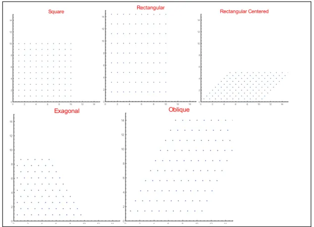
The two dimensional continuum bodies are discretized into a finite number of particles occupying, in their initial configuration, the nodes of a lattice. The kind of lattice is chosen between the five plane Bravais lattices as you can see in Figure 2 but sometime could be useful to use also honey comb lattice. This is the first choice we have to

do (Choice 1); changing lattice, and other parameters we shall see later, as we can obtain different results with the same initial conditions.

Figure 2 Bravais plane lattice

In Figure 3 a discretization example is shown.

Figure 3 Example of discretized object in the chosen lattice with frame (yellow points). Square Lattice have been used

0 2 4 6 8 10 12 14 0 2 4 6 8 10 12 14 Square 0 2 4 6 8 10 12 14 0 2 4 6 8 10 12 14 Rectangular 0 2 4 6 8 10 12 14 0 2 4 6 8 10 12 14 Rectangular Centered 0 2 4 6 8 10 12 14 0 2 4 6 8 10 12 14 Exagonal 0 2 4 6 8 10 12 14 0 2 4 6 8 10 12 14 Oblique 20 40 60 80 100 120 20 40 60 80 100

We consider four kinds of particles but it is possible to generalize introducing new kind of particles, to enlarge our description possibilities, owing the modular structure of the algorithm. Moreover the role of the particles can be dynamically changed during body’s deformation. They are:

1. The leaders; their motion is assigned and determine the displacement of the other particles (i.e. they represent the imposed strain of part of the body).

2. The followers; their motion is determined by the interaction rule with other particles.

3. The frame; it is introduced so that any particle has the same number of neighbors, to avoid edge effects. The motion of the frame particles is determined by the frame rule (see Figure 4 and 5).

4. The ghost; this particles are introduced to describe fracture mechanism. (see Figure 6) The displacements of the leaders is assigned so does not need any explanation.

How we determine the displacement of the followers? First we have to choice the neighbors of any particles (Choice 2). Typically we used the firs nc particles, where nc is the coordination number of the lattice. This is the case of first gradient theory; but we can choose to use a larger set of neighbors, like the neighbors of the neighbors and this is the second gradient theory case. So far we enlarge the set of points with a supplementary shell and this can be generalized to nth order interaction (see Figure 4 and 5).

Later we have to choice the interacting rule (Choice 3) between the particles. The rule describes the position of a particle as function of the neighbor’s positions. As example we can decide to use the centre of gravity rule where the new x coordinate of the particle j is

𝑥

(𝑡) =

𝑎𝑙𝑙 𝑛𝑒𝑖𝑔ℎ𝑏𝑜𝑢𝑟𝑠 𝑜𝑓 𝑗 𝑘=1

𝑁

(1)

Where N is the total number of neighbors; similar equation can be used for the y coordinate. By this way displacement of a follower point is the average value of the displacements of its neighbors; the number of shells determine the order of interaction. We can use different rules in order to imitate different constitutive equations. Possible generalizations of Eq.1 are geometric, power and weighted mean. Possible weight is the particles Euclidean distances dis(k,j) between the particles k and its neighbor j. This can simulate Hook law, where recalling force is increased with increasing deformation. By Eq.1 we note as x and y coordinate are independent so Poisson effect cannot be obtained. A possibility to obtain it is to use

𝑦

(𝑡) = 𝐾 ∗ (𝑥

(𝑡) − 𝑥

(𝑡

)) ∗ 𝑑𝑎 +

𝑁

(2)

Where da is a function of the distance from the central axis, K a parameter determining the response force and

x(t0) the x coordinate at time t0. So far expansion of x coordinate has effect on the y coordinate. The Euclidean

distance, dis(k,j), can be used as weight.

𝑥

(𝑡) =

𝑎𝑙𝑙 𝑛𝑒𝑖𝑔ℎ𝑏𝑜𝑢𝑟𝑠 𝑜𝑓 𝑗 𝑘=1

∑𝑎𝑙𝑙 𝑛𝑒𝑖𝑔ℎ𝑏𝑜𝑢𝑟𝑠 𝑜𝑓 𝑗_𝑘=1 𝑑𝑖𝑠(𝑘,𝑗)

(3)

We can also force the follower’s movement to overcome the barycentre equilibrium position, leading the lattice to oscillate.

𝑥

(𝑡) =

+ 𝑓𝑑 (

− 𝑀𝑇(𝑗, 𝑡

)) (4)

Where w(k,j) is the weight, fd is a feedback factor and MT(i,t0) is the x-coordinate of j point at t0 to have memory

of the initial configuration.

The compute of new position for a particle set can be considered as a constrained geometrical problem using a transformation operator between the matrices describing particles configuration, Ct, for a discrete set of time steps

t1, t2, ...tn...

In our algorithm, the neighbors can dynamically change at every time step. Actually we choice to fix the neighbors of every particle at the initial time t0, and not to change them during time evolution of the

configurations; this has the mean to consider a crystalline lattice and therefore to deal with solid phase materials. The concept of neighbors is Lagrangian, and neighborhood is preserved during the time evolution of the system; the only exceptions arising with the fracture algorithm, as shown later. Also the definition of neighbors is customizable by changing metric; for example we can consider points whose Euclidean distance (weighted or not is another possibility to take into account anisotropies) is less than a threshold, instead of the coordination number of the lattice.

Starting from the leader’s motion each time step the displacement propagates of one shell, determined by the neighbors up to involve all the particles.

To avoid edge effects we build a frame surrounding the body by an external shell of point, so that any follower interacts with the same number of elements. Our objective is homogeneity of the boundary conditions for all the

followers. Without the frame a corner point has fewer neighbors, with respect to an internal point; so far if its coordinates are determined, as example, by barycenter of its neighbors this point will be attracted toward the inside and the lattice and will collapse on the other points.

Figure 4 Kind of particles

Figura 5 Kind of particles (2° gradient case)

The motion of the frame is simple: it only has to follow the motion of an assigned follower of its competence; in case the assigned followers are more (i.e. in a corner) then an average displacement, or a more generic complex rule (Choice 4), is considered as can be seen in Figure 5. In this case you have more than a possibility and the frame can be something more complex than a single shell; as an example if we are considering second gradient interaction we need a double shell to reach. Later we shall see as in hexagonal lattice you can choose more than one kind of frame and the obtained results are completely different.

The process stops when all the elements of the system have moved, and then restarts at every following time step (for a more detailed description the reader is referred to [21], [97]).

The model exhibits pronounced nonlinear behaviors, as shown in [61], since composing motions for the leader does not lead to a simple superposition of effects in the configuration of the system.

To manage fracture phenomena we assume the interactions are decreasing with increasing distance between particles. Therefore, when Euclidean distance between points is “great”, they lose their interaction. To address the problem we start simply considering a threshold effect between neighbor elements, so that when the distance overcomes the threshold these elements stop to influence each other so they are no longer taken into account in the calculation of the follower position. To preserve symmetry of the Lagrangian neighbors we introduce ghost points with the purpose of balancing the calculations of the point’s displacements, just to balance the equations. They have the purpose of balancing the calculations of the point’s displacements. Where are these ghost elements posed? Typical position, where we put ghost points (Choice 6), is that is able to recover the original shape of the lattice (see Figure 6). Anyway other choices lead to different results. All the properties of these ghost elements are

the same of the followers but their motion is not considered, because they are not in the list of the followers. They are just in the right position to balance the cell. As we have seen [99] a change in their position produces effects such as the contraction or loosening of the lattice in the deformed configuration. In fact, varying the distances of the ghost elements after fracture from the true elements, plastic-like and elastic-like behaviors can be obtained. As elastic behavior in fracture we mean the property of the fracture edges or of the disconnected pieces originated after fracture has occurred, to recover its original shape. The algorithm can be easily generalized to second gradient by introducing two different thresholds for the two shells of neighbors.

Figura 6 Fracture mechanism: ghost

Practically you have to decide constrains of the lattice and the interaction rules between the followers, in order to describe the correct behavior of the constitutive equations of the materials.

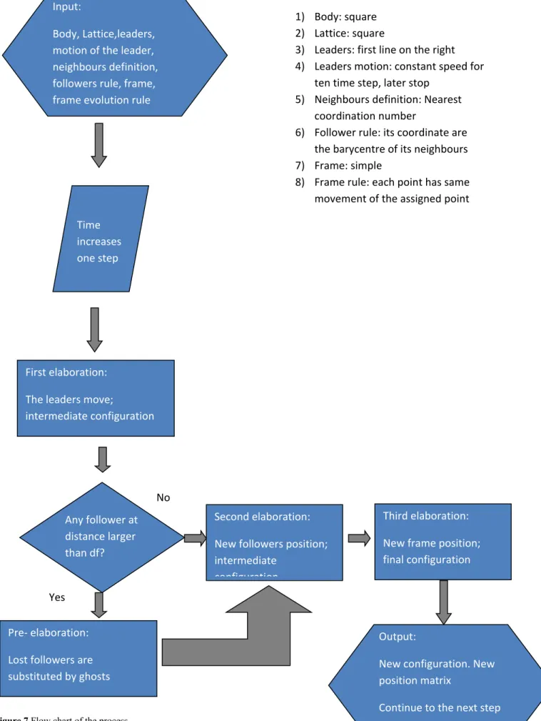
Reassuming the process is the following (seethe flow chart in Figure 7). We choose a two dimensional body and one of the Bravais lattice and discretize it to obtain a discrete matrix to represent it. We now decide the constrains of the lattice and the interaction rules between the followers, in order to describe the correct behavior of the constitutive equations of the materials. As an example we can decide that the lattice has no constraints and displacement of a follower point is the average value of the displacements of its first neighbors (first gradient). We build an adequate frame to avoid board effects. We decide the motions of some points, called leaders, for all the time windows we are investigating; we can also decide that they will be leader only for a certain time and late become followers (Category change).

Now we can calculate, for each time step, the new configuration of the lattice in three separate operations. When time increases from t0 to t1 the leaders change their position from initial configuration according to the prescribed

equation. So far we build a new intermediate lattice where only the leaders have been moved. Now we take care that the followers are no longer in equilibrium position owing to the leader’s displacement. How we can calculate it? As an example if the interactions rule establishes that a follower has to be in the barycenter of all its neighbors we calculate the new position of each follower, taking into account the leader displacement. So far note as at this stage only the leader’s neighbors are involved. Finally we take into account the rules governing the frame displacement. This is our new configuration at time t1. It is important to note as reached the configuration is not an

equilibrium one, because the three operations must be repeated for many time step, after the leaders stop. To be more clear if at time step one the leaders have moved we calculate the follower’s displacement. This operation involves only the neighbors of the leaders and not the other far followers. Later we calculate the frame displacement to close the loop. Now there are some followers (the neighbors of the leader’s neighbors) that there are no longer in equilibrium because there has been the displacement of the leader’s neighbors. So we need another time step to adjust the configuration and so on. At a certain time all the followers are involved in the calculation. The followers will suffer the leader’s motion after (k-1) time steps where k is the distance from the leaders, measured in layers. In this meaning the leader motion “propagates” through the lattice to influence the position of all the followers in a time depending on the lattice dimensions and how many shells of points are being considered in the neighbor’s definition. In the same way when leaders stop the followers continue to adjust their position in many time steps.

At this point we can open a long discussion on the concept of time which is present here only as “step”. So our question is concerning if we have to consider some virtual configuration between time ti, and ti+1, until the

equilibrium is reached or not. In the second case, we have used in this work, the second movement of the leaders happen when the second shell of neighbors is just interested from the first displacements of the leaders. There are some conceptual differences in the two methods we are still investigating.

Figure 7 Flow chart of the process

Input:

Body, Lattice,leaders, motion of the leader, neighbours definition, followers rule, frame, frame evolution rule

Time increases one step

First elaboration: The leaders move;

intermediate configuration

Example of assignment: 1) Body: square 2) Lattice: square

3) Leaders: first line on the right 4) Leaders motion: constant speed for

ten time step, later stop 5) Neighbours definition: Nearest

coordination number

6) Follower rule: its coordinate are the barycentre of its neighbours 7) Frame: simple

8) Frame rule: each point has same movement of the assigned point

Third elaboration: New frame position; final configuration Second elaboration:

New followers position; intermediate

configuration

Output:

New configuration. New position matrix

Continue to the next step Any follower at

distance larger than df?

Pre- elaboration: Lost followers are substituted by ghosts

No

In the next future we are considering the possibility to discuss the proposed model in a fully variational setting, which is by no means trivial but would provide clear methodological advantages (see [100] for an introduction and [101]–[105] for illustrative cases concerning continua with non-classical properties); therefore we like to introduce pseudoenergetic considerations by two formulations PE1 and PE2 to give a contour plot of the strain distribution. The first is the sum, extended to the neighbors, of squares of the differences between the distances of the point from its neighbors minus the distance in the initial configuration i.e.

𝑃𝐸1(𝑡, 𝑗) =

∑

(𝑑𝑖𝑠(𝑡, 𝑘, 𝑗) − 𝑑𝑖𝑠(𝑡

𝑘, 𝑗))

𝑎𝑙𝑙 𝑛𝑒𝑖𝑔ℎ𝑏𝑜𝑢𝑟𝑠 𝑜𝑓 𝑗

𝑘=1

Where dis(t,k,j) is the Euclidean distance between points k and j at time t. The reason for this choice lies in the attempt to emulate potential energy of material point subject to Hook law. It is a sort of square distance between the actual configuration Ct and the reference configuration C0.

To compare time contiguous configuration Ct and Ct-1we define for each point j and each time t

𝑃𝐸2(𝑡, 𝑗) = ||𝐶

− 𝐶

||

Where || is the Norm of the vector defined by the point j at time t and t-1.

It must be underlined that this artifice has no direct connection with the usual energy definition (this is the reason we use the term pseudoenergy) but could be useful to understand deformation.

Moreover, an algorithm based on the geometric barycenter of the neighbors of a given particle is consistent with the idea of locally minimizing an elastic potential, as the centroid has the well-known properties of minimizing the sum of the squared distances from a set of given points in an Euclidean space. Therefore, the proposed algorithm seems a natural discrete approach from the variational point of view. Another possibility, close to these concepts, we are considering is to substitute Eq. 1-4 by potential field able to determine particle displacements and avoid collisions.

5. Some examples

Aim of this section is to show the coherence of the model and its adaptability in showing different physical phenomena by changing some parameters. Therefore we approach some bidimensional problems relative to simple shape object subject to imposed strain of some leaders which are significant; for some of the tests we shall show and discuss the movement of the particles, the XY movement of a significant particle (if present) and some pseudo energetic considerations by PE1 or PE2. See preceding works [21], [97], [99]. The behavior of some more complex ASTM samples and the respect of Saint Venant principle have also been described; moreover, looking for the limits of the tool, we shall discuss some not satisfactory results.

Case a1) Simple stress test

This was the first simple test we have investigated. Consider a square shape specimen subjected to pull and release in tensile test. We are considering a sample undergoing strain from one side (the other side is clamped) at constant velocity in x direction (speed 0.6 unit length/step time), with a square lattice 10x10 particles unit. At a certain time the pull is released and the leaders return to original configuration (this means that leaders have changed category and now they are followers) attracted by the other points. The simple rule, governing follower’s motion is that every point must be placed in the barycentre of its neighbors (Eq. 1); the neighbors’ are determined by the coordination number of the square lattice; therefore the leader’s motion implies a displacement of the first layer that propagates in successive time steps to the other particles. Therefore the displacements, at each time step, involve a larger shell of points until to regards all the lattice points. In second gradient [5-7] we consider also the neighbors of the first neighbors’. In Figure 8 we can see the configuration of the lattice over different time together with the PE1 contour plot. Red points are the leaders; blue the followers and orange the frame. From the figure we can outline that the x displacement of the points seems do not depend on the y coordinate; however looking at the PE1 picture we can note a light convexity that does mean this is not true.

Figure 8 Configuration of the lattice over different time (1,10, 20 and 401) and PE1 contour plot

A deeper examination of the point’s displacements confirms as close to the frame the displacements, along x coordinate, are lower with respect to central points. This can be explained as an edge effect. In fact if we consider points on the same vertical lines those that are close to the frame follow the neighbors with a little delay owing to the different rule determining the displacement of the frame and of the followers. So they see a different situation with respect to a central point. Moreover we can note as the maximum value of PE1 (red area) is not on the leader line but just one line on its left; this because, in this case, the leaders have in their neighbors, some points of the frame that always are close to them. We can avoid this convexity effect using a different frame or mirroring the followers to obtain an infinite sample. This is also evident in Figure 9 where contigue configurations are compared using the PE2 formula.

Figure 9 Configuration of the lattice over different time (equivalent to 2 and 10 of PE1) and PE2 contour plot

Now we put attention on a single point of the lattice. Consider a central point j=67 (sixth column, seventh row, points are numbered from left to right and from bottom to up). The value of the PE1 increases notably when points are pulled, after a delay owing to the propagation time as can be seen in Figure 10 and Figure 11; it decrease when the leaders become followers subjected only to the rules leading to equilibrium barycentre position. If we change point the shape of the curve remains the same but can be less o more flared as can be seen in Figure 12 and 13 where we consider a point closer to the leaders (j=115). Also in this picture we can recognize the coordinate x increases linearly (velocity is constant), after a delay (less for j=115), owing to the propagation time and later decrease to the original position.

Figure 10 PE1 of the central point’s j=67 versus time Figure 11 X Evolution of the point j=67 versus time

Figure 12 X Evolution of the point j=115 versus time Figure 13 X Evolution j=115 versus time (modified rule with

feedback)

A light modification can generate instabilities and oscillations; as example we can add to Eq.1 a feedback term proportional to the difference between actual and initial position to overshoot the old equilibrium position. The result is showed in Figure 14 and Figure 15 (we used different feedback); note as also the reaction time is changed. Using higher feedback instabilities can be generated (see Figure 15).

Figure 14 X Evolution j=115 versus time (modified rule with feedback) Figure 15 X Evolution of the point j=67 versus time

(modified rule with feedback) Case a2) Poisson effect

In the second case we change the interaction rules; the case is the same as the preceding (without release, the leaders stop after movement and the motion steps are 100) but the follower position is determined not only by a baricentric equation but the rule take into account the other coordinate. We call this method “mixed coordinate”. In Figure 16 we can see the configuration of the lattice over different times together with the PE1 contour plot.

Figure 16 Configuration of the lattice over different time (1,10, 20 and 100) and PE1 contour plot

Lateral contraction can be seen. Note that there is a relaxation time, because the followers need time to adapt themselves. This is due to the rules expression and can be tuned as you desire. The PE1 value seems to follow the configuration; here is more evident the edge effect leading to concavity effect toward left side.

In Figure 17 we can see the configuration of the lattice over different times together with the PE1 contour plot in second gradient case. In second gradient case lateral contraction can be seen in a less pronounced way; this is because if we take into account a larger number of neighbors the effect is dumped. The PE1 plot enhances the convexity of the first line of follower. We shall see better as, in the fracture case, second gradient has much more influence in some other cases.

In Figure 18 and 19 the evolution with time of central point j=67, is shown and the lateral contraction, in y coordinate, is evident. The point is above the central line so their y coordinates decrease. Note as the second gradient case show a less pronounced effect on y coordinate.

Figure 17 Configuration of the lattice over different time (1,10, 20 and 100) and PE1 contour plot. Second gradient

Figure 18 Evolution of the central point j=67 versus time

Case b1) Shear test

We now consider a shear test to evaluate the influence of the lattice type, of the interactions rule and of the second gradient neighbors on the deformation obtained. The specimen is subject to a shear with constant velocity 0.1 unit/time step in x axes, by the leaders. We consider 100 time step of strain. As usual when we do not have specified interaction rules between the followers we use the barycenter rule i.e. the coordinate of the follower is computed as the gravity center of all its neighbors. Moreover, if not specified, the number of neighbors is given by the coordination number of the chosen lattice, while in second gradient there is a second shell. No fracture is still considered in this case.

In Figure20 we can see the configuration of the lattice together with the PE2 contour plot, to compare contiguous configurations. As usual the leaders are red, the followers blue and the frame is in orange color. Lateral deformation are non linear and comparing contiguous configuration, by PE2 function, differences are larger close to the leaders. No deformation of the top and bottom line can be outlined.

Figure20 Configuration of the lattice over different time (2, 45, 85 and 100) in shear test square lattice together with PE2 contour

plot, indicating differences between contiguous configurations.

A more marked lateral deformation curve can be seen if we use a honey comb lattice (see Figure21). This is an example of how different deformed configurations can be obtained by changing lattice type holding all the other conditions. We remark that this is not a Bravais lattice but we have used it owing to its large practical applications. As in the previous case PE2 contour plot shows that differences between contiguous configurations are larger close to the leaders

Figure21 Configuration of the honey comb lattice over different time (2, 45, 85 and 100) in shear test square lattice together with

PE2 contour plot, indicating differences between contiguous configurations.

A more interesting case, using a square lattice, is shown in Figure22. Here we have used a rule for the follower making use of “mixed coordinate”, which means the y coordinate is dependent on the evolution of the x coordinate. This allows us to obtain lateral contraction, i.e. Poisson effect. The result of the shear test is a strange “window” flag. Once again PE2 contour plot show that large differences between time contiguous configurations can be outlined close to the leaders, from no particular differences with the preceding plots.

Quite similar behavior can be observed if we use second gradient model, changing the shell of neighbors). Differences are in a more stiff reaction, owing to the larger numbers of neighbors involved in calculating the follower’s positions.

Figure22 Configuration of the lattice with Poisson effect over different time (2, 45, 85 and 100) in shear test square lattice together

with PE2 contour plot, indicating differences between contiguous configurations.

Case c) Saint Venant

In this case we shall verify the local action principle, whereby the tension at one point is not influenced by the motion of the external particles to an arbitrarily small circle of the particle in question. To this aim we consider four internal points that diverge from their initial configuration; practically we choose four internal points as leaders with opposite movement along the bisectors of the corners. In Figure 23 we can see the configuration of the lattice in different time together with the PE1 contour plot. As can be seen remote particles are not interested in what is going on close to the leaders.

Figure 23 Configuration of the lattice at time (9) with PE1 and PE2countour plot

Case d) Fracture test

For the next example we shall consider a square sample undergone a tensile test with fracture. Fracture distances are 10 units and speed is 0.5 units/step, for 150 steps long. When a distance between the points is larger than fracture distances the sample is broken and the followers go to equilibrium position; if no followers remain attached to the leaders (it depends on the distances, we shall see later in other cases) they return to their initial

position. As explained in a preceding work [21], [97], [99]the convexity, in the fracture mechanism, is related to the presence of the frame. Analysis of PE1 plot show as, before fracture, there are areas of stress concentration. Higher stress areas are close to the leaders. The trend of the follower points is quite linear during traction but it becomes non linear when the followers remain alone and return back. This can be explained because the traction is imposed with constant speed, while the reassembly of the points is driven by the follower’s rules. Once again involving a larger number of neighbors lead to a more stiff behavior as can be seen in Figure 25 (second gradient case). We can see as the vertical fracture line is different in the case of first (see Figure 24) or second gradient (see Figure 25). Points close to the frame are detached before the others from the leaders, and this effect is more marked in second gradient case. This can be explained with the different neighbor’s number and also with the larger influence of the frame with respect to the first gradient case.

Figure 24 Configuration of the lattice over different time (1,5, 6,7 and 100) and PE1 contour plot, fracture in tensile test. First

gradient

Remember that in the fracture case the pseudo energy plot is less indicative, because we are calculating it using distance between points greater than the fracture threshold. In a future work we will consider a better definition of this parameter.

Figure 25 Configuration of the lattice over different time (1,5, 6,7 ,8 and 100) and PE1 contour plot, fracture in tensile test. Second

gradient

The importance of second gradient must be outlined in Figure 26 where x coordinate evolutions versus time of x coordinate of point 103 is showed. The point is situated in middle value as Y coordinate and two lines on the left of the leader’s line; differently from first gradient mode a complex behavior can be observed because after the fracture the x coordinate has a sort of rebound. This can be explained as follow. After the fracture the point try to return its initial position (on the left), but later some fast point on its right try to deviate it to the right. When the group is compacted they go back all together to initial configuration. So far change in the parameters can lead to complex evolution behavior of the lattice.

The fracture mechanism is strongly dependent on lattice characteristics; in the next case we use a hexagonal lattice, instead of square. In this case we can choice two different rules for the frame, as can be seen from Figure 27. In the first case a frame point displacement is just the same of the corresponding follower. But in some case, like hexagonal lattice, you can decide there are more than one corresponding followers and choice the point frame displacement as the average value of them. The behavior is very different from the square lattice case as we expected. It can be noted that a point of the frame remains in the middle of the displacement, if we use the average value. This can be explained as follows. The rules regarding the frame are simple; each point of the frame is linked to an assigned follower and its displacement from time t to t+1 is the copy of the follower. However in some cases the followers assigned to one point of the frame could be more than one. In such cases we can choose

to take one of them or to consider the displacement of the point as the average value of the displacements of all its followers linked to it. This is the reason that two points of the frame remain in the middle: they are stressed from two opposite sides. The behavior is very interesting; it can be noted that a different equilibrium configuration is reached because the frame is changed and the fictious, introduced to manage fracture, are not in the list of the followers. In the case of Figure 28 this results in a concave final surface, owing to the modified frame.

Figure 26 Evolution of the second follower line point j=103 versus time

If we use the other frame rule the fracture is similar to square lattice. This lead to different final deformed configuration as can be outlined in Figure 28. The presence of a frame point in the middle leads the final configuration to a concavity. The absence of followers on the right side, once again is depending on the leader’s speed.

Figure 27 Alternative choice for the frame rule displacement. In the first case each frame point is moving as a corresponding

Figure 28 Configuration of the lattice over different time (1,7,8,9,10,12,27 and 400) and PE1 contour plot

A rebound mechanism can be outlined from Figure29 and Figure 30. This is typical of a hexagonal lattice; you can note that in the square lattice this behavior does not exist.

Figure29 Evolution of the central point j=133 versus time; first and second gradient, see Figure 28 and 30

Also in this case second gradient mode attenuates the effects, see Figure 30. No rebound can be outlined and the equilibrium configuration, after the fracture is similar to the original. Cuspidal point in X coordinate, after about 100 step, can be attributed to a second fracture happening.

Figure 30 Configuration of the lattice over different time (1, 7, 8, 9,10,12,27 and 401) and PE1 contour plot

Finally in Figure31 fracture mechanism of simple square lattice under shear stress is shown. It can be noted that the leaders bring with them some of the followers; this depends on a complex balance between the leader’s attraction and the resistance offered by the followers. Changing condition results in changing the number of the “attached” followers. After the fracture the particles return back to their equilibrium position. Note that if we would position the fictitious in another location we would obtain a different result. Pseudoenergy has symmetric behavior, as expected. Remember that the pseudoenergy concept was considered on not fractured sample, and it is not calculated on the fictitious points but on the followers so it is not significant.

Figure31 Shear Configuration of the lattice over different time (2, 45, 85 and 114) in shear test square lattice with fracture together

with PE1 contour plot, of pseudoenergy.

Another example can be obtained if we consider a rectangular centered lattice but we the neighbor’s number, nc,

to five and consider a first gradient interaction; we obtain a completely different result. In Figure32 we have a tensile test as the preceding; the lower number of particles involved in the calculation of the relative position makes the sample much more fluid, allowing detachment of a larger number of particles, as we can see on the right side of the pictures. The fracture mechanism also is different with respect to the preceding case.

This gives more mobility to the model leading to a more plastic behavior and increasing the number of the detached points; the fracture mechanism is quite different together as well as the final configuration (see Figure 32). This example shows, once again, that change in model parameters lead to different behaviors.

Figure32 Tensile test with fracture rectangular centered lattice, coordination number 5. Configuration over different time (1, 23, 33,

38, 40 and 63) with PE1 contour plot, of pseudoenergy.

An interesting phenomenon can be seen if we consider an oblique lattice (Figure 33). Owing to the asymmetry (see look at the five red leaders on the right) of the leaders with respect to the frame a particular breakage fracture can be observed. In fact if we consider a symmetry axes in x direction we can note two leaders close to the frame in the upper level and only one close to the bottom. This leads to a fracture starting from the bottom where the attraction of the leaders is lower. It seems to rip a piece of paper. The fracture distance is 10 units and the speed is

0.4 unit/time step.

Figure 33 Oblique lattice tensile test. Red points are leaders, blue point followers and yellow the frame. First gradient case. Note the

Figure34 Tensile test with oblique lattice: breakage fracture. Configuration over different time (1, 32, 55, 82, 90,101,113 and 200)

with PE1 contour plot, of pseudoenergy

Case c) ASTM test

In order to investigate sample behavior of a well known shape we have carried out some calculations considering a specimen quite similar to the ASTM D638 standards for tensile tests. The specimen is clamped at both ends on a

surface and pulled on one side, so, in this case, the leaders are many; the test speed is of 2.5 unit/step, in x positive direction, for 150 traction step e 2500 relaxation step. We have considered simple tensile tests with different lattice, lateral contraction effect and fracture cases. Generally a larger number of time steps is required for relaxation, owing to the larger number of points employed to describe the specimen; this does not mean a longer relaxation time, because unit time is arbitrary, only that the influence of the displacement propagates at one shell (first gradient case) each time step so we need many steps to involve the whole sample. Once again the second gradient case seems to be stiffer with respect of the first gradient.

It should be noted that, in our pictures, the sample does not reach a symmetric final configuration as we can expect because of the long time required.

If we consider the simple tensile tests (see Figure 35 and 36) little quantitative differences in point distribution can be observed during the classical elongation of the specimen in different cases. We can observe differences in the internal distribution on the points and in the convexity of the propagation front of the deformation (see Figure 41) i.e. see the convexity of the points between the two figures We are working on this and on higher gradient computations.

On the contrary if we use a rectangular shape sample it does (the points are equally spaced) as can be seen in Figure 37. There is no physical reason for this, our opinion is that this effect is linked to the particular equilibrium condition generate by the geometry. It can be outlined as final configuration is more similar to a symmetric one, in second gradient case, owing to the larger number of points involved in the computation.

In the two cases we are considering the Poisson effect (Figure 38 and 39) it is possible to see lateral contraction. It seems the points cluster to create islands but this effect must be investigated better. In case of second gradient interaction this does not occur, as can be seen in Figura 39. The fracture test (see Figura 40, Figura 41 and Figura 42) is considered for the rectangular centered lattice. Distance fracture is 11 units and the speed was 0.6step/unit time. As can be seen, the fracture occurs close to the top of the profile and not in the central area. Studies, in progress, show as the fracture zone can be moved by varying working conditions. We can render the fracture more or less brittle changing the model parameters like neighbors’ number, type of lattice, speed etc. As example in second gradient the same sample has a more brittle behavior; or if I use a speed of 2.5 step/unit time in the same condition I will get no followers on the right side of the fractured sample. We can observe differences in the internal distribution on the points and in the convexity of the propagation front of the deformation i.e. see the convexity of the points owing to the different lattice used compared to the preceding case.

Figure35 ASTM tensile test square lattice. Configuration over different time (1, 40,160, and 2500) with PE1 contour plot, of

Figure36 ASTM tensile test rectangular honey comb lattice. Configuration over different time (1, 40,160, and 2500) with PE1

contour plot, of pseudoenergy.

Figura 37 Rectangular sample square lattice

Figura 38 ASTM sample Poisson effect square lattice

Figura 40 ASTM rectangula centered lattice before tensile test

Figura 41 ASTM rectangula centered lattice after tensile test

Figura 42 ASTM square lattice fracture

Case h) Short beam, the plate

Now we want show some differences between the solution of a bending plate undergoing a shear load and what we have obtained by our tool. In the preceding works we got some success but we need to go deeply to a better understanding so we are looking for some cases that do not fit on what we are expecting. We consider a bi-dimensional square plate (X and Y coordinate from 10 to 21) with materials parameters Y=1000 and ν=0.33, where Y is the Young modulus, ν the Poisson coefficient; boundary load is on the right (Neumann condition) and no displacements on the left (Dirichelet conditions).

The equations to be solved are:

Y 2(1 + ν)∇ 2_{𝐮 +} Y 2(1 − ν)( 𝜕 𝜕𝑥𝐮 + 𝜕 𝜕𝑦𝐯) = 0 Y 2(1 + ν)∇ 2_{𝐯 +} Y 2(1 − ν)( 𝜕 𝜕𝑥𝐮 + 𝜕 𝜕𝑦𝐯) = 0

u(x,y) and v(x,y) are the displacements function. We pose as boundary conditions 50 Pascal as shear stress on the plate (Neumann condition for x=21) and u(10,y)= v(10,y)=0 as Dirichelet condition. Note that we are using Bernoulli equation while Timoshenko model should be more appropriated. Anyway this is just a first attempt so we reserve the right to use it in a next paper. These equations can be solved numerically; if we discretize our plate by a 10 x 10 square lattice; the solution is shown in Figure 43 and the Von Mises plot in Figure 44; deformed mesh are plotted in red colour.

Figure 43 FEM solutions of bidimensional square Figure 44 Von Mises plot of FEM solutions

beam under shear stress

Our intention is to compare the strain of the plate, obtained by FEM solutions, with that we can compute by our tool. Therefore we have to assign the displacements of some points, the leaders, make some choice about the algorithm (Lattice, interaction rules between the followers etc..) and compute the strain when the followers readjust themselves, after a while. As leaders we choose the right and left side of the plate, so we impose the displacements of these points as computed from the FEM equations and investigate the arrangement of the other points. It is important to remark that we have no criteria about the choice of what lattice, interaction law between followers etc... So as first attempt we use a square lattice and no weight in the computational of the followers coordinate In Figure 45 the obtained configuration, together with the FEM solution (red points) are shown; in Figure 46 the corresponding Von Mises plot. The points on the left and on the right of the plate are overlapped because are the leaders and we have imposed their displacement as the FEM solution of the plate deformation. It can be outlined as external configuration of the plate is quite the same but the internal displacement of the points, i.e. the strain, is different; this can be highlighted if we plot the Von Mises stress. Change in tool’s parameters lead to different configuration, corresponding to different strain of the plate, almost none of them are satisfactory as shown in the following pictures. Second gradient case has showed no appreciable differences; we have tried to give a quantitative measurement of the discrepancies with the FEM solutions, using the average value of the sum of the square differences between coordinates, in many cases. Nobody emerges as the best match so we can conclude that the plate deformation can be sometimes very similar to the FEM solution but the Von Mises stress plot is quite always unsatisfactory. This point need to be study again to a better understanding of the physic behind the tool and what should be drive our choices in the tool to describe material continuum. We have to remember that the materials parameters Y and ν does not appear explicitly in our algorithm but they are hidden into the interaction relationship between the followers, the neighbours and the choice of the lattice. So far we have no idea on how to select our choices to match the well known problem. Changing the parameters of our tool we obtain different results nobody of them perfectly coincident with classical solution but, owing to the flexibility of the tool, we believe it exist a parameters combination to fit the deformed beam; but this is meaningless until we do not understand how to choose the parameters.. The reason of this lie in the fact that, up to now, we do not start from the constitutive equations of the materials leading to the rules governing points displacement. We have to work on how to connect the rules of our model with classical physical proprieties of the material.

Figure 45 Beam deformation Figure 46 Corresponding Von Mises Plot

In Figure 47 and Figure 48 we are considering the case with square lattice, first gradient and we used power mean in Eq.1 with power factor -1 (harmonic mean). Here a strong difference with the FEM solution (red points) can be noted but similar to the Timoshenko Beam deformation shape where the cross sections, perpendicular to the neutral axis before deformation, stay plane after deformation but are not necessarily perpendicular to the neutral axis after deformation. This was expected because the -1 power parameter changes deeply the Eq.1 into the following equation: 𝑥𝑗(𝑡) = ( ∑𝑎𝑙𝑙 𝑛𝑒𝑖𝑔ℎ𝑏𝑜𝑢𝑟𝑠 𝑜𝑓 𝑗𝑘=1 (𝑤(𝑘)𝑥𝑘(𝑡))𝑝 ∑𝑎𝑙𝑙 𝑛𝑒𝑖𝑔ℎ𝑏𝑜𝑢𝑟𝑠 𝑜𝑓 𝑗𝑤(𝑘)𝑝 𝑘=1 )1/𝑝

Where w(k) is the weight, in this case 1, of the k-element and p the mean parameter, -1.

Figure 47Plate deformation Figure 48Corresponding Von Mises Plot

In Figure 49 and 50 we are considering honey comb lattice that sounds as one of the best result.

Case i) Long beam

Also in the case of longer beam we can try many combination of the parameters tool to fit the deflection of our beam but it is useless: we need to connect the constitutive parameters with the tool. If we increase the ratio length/width of our beam from 1 to 5 the results are still different (see Figure 51,52,53 and 54)). As can be seen the results do not behave as we expected and show a wide range of possibilities in which we could choose. Similar results were obtained if we increase the ratio length/width up to 10 or more. Although the external shape of the beam can sometimes be acceptable, once again we can see as the displacement of the internal particles is quite different from the FEM solutions; it is clear that the differences are sometimes noticeable, as outlined by the Von Mises' graphs. So far we stop trial and errors to think about a better understanding of the physic behind the tool and what should drive our choices in the tool to describe material continuum. This will be the object of the next paper.

Figure 51Square lattice Figure 52 Square lattice reduced neighbors numbers

Figura 53 Hexagonal lattice Figure 54 Hexagonal lattice reduced neighbours numbers

6. Future work

The presented results are interesting but they still are at a preliminary stage. We have collected some success showing plausible deformation in different conditions but when we consider a beam under loading the need to connect constitutive equations with the parameters of our tool emerges powerfully. We have stressed what still need to investigate as a beam under shear stress. Changing the parameters of our tool we obtain different results nobody of them perfectly coincident with classical solution. The reason of this lie in the fact that, up to now, we do not start from the constitutive equations of the materials to obtain the rules governing points displacement. So far the most important topic to be investigated is concerning how to relate materials parameters with the choices we are doing in our tool. This must be done to achieve a connection with the usual methods of Continuum Mechanic. As matter of fact we, actually, have not criteria about how direct our tool’s choices to describe a particular material continuum. In the beam deformation we have assigned Young modulus and Poisson coefficient but there is no relationship between them and the parameters of our model i.e. the follower’s rules. This is the reason of the discrepancy in the resulting deformation compared to FEM solution.

Generalization in 3D of the tool is quite easy but still needs some optimization in the code to keep the computation time in the order of seconds, by using a normal PC Desktop.

We are relaxing the hypothesis that the neighbors always are the same to describe liquid and gas; this needs an intermediate calculation step because you have to compute who the neighbors are, defined in this case as the particles inside a specified volume, at each time step.

We are introducing constrained on the particle’s motion to describe structured object like pantograph [106]–[113] . It can be described as a set of beams with constrained point in the pivot or, in the Hencky vision, can be conceived as a set of points interconnected by springs.

Further developments are concerning different fracture mechanism, different frame to avoid edge effects, other interactions rules and adaptive lattice.

A generalization of the interaction algorithm, to encompass the richness of behavior of different materials like metal or plastic is auspicable, including potentially complex biological tissues [114]–[118]. An appropriate potential interaction could take into account different deformation regimes, such as elastic and plastic ones together with fracture. To this aim pseudo energetic considerations are introduced also to achieve a better understanding of the process. This is preliminary to introducing potential descriptive interactions depending on the relative distance between the particles, which are able to reproduce the well known physical behavior.

Cellular automata seems to be a good candidate to enhance our work; A cellular automata is a simple computational mechanism that, for example, changes the color of each cell on a lattice based on the color of neighbors’ cells according to a transformation rule. Some attempts, to use them in Mechanics have been done [119], [120]. Principal limit of Cellular automata is regarding as do not evolve sufficiently, so they quickly reach a limited asymptote in their order of complexity and this will be the object of a future paper. An evolutionary process involving conflict and competition is needed, like in biology systems to overcome this difficult. Moreover there is no way to predict the outcome of a cellular process without actually running the process. So even though our decisions are determined, there is no way to predetermine what these decisions will be. But the system has succeeded, especially in fluid dynamics to describe complex behavior. The question posed about if I can work on patterns of information, rather than matter and energy, represent one of the more fundamental building blocks of reality is still open and we would like to make a connection with our tool.

Moreover how stable and robust is the model? What is possible to describe with this model and what are the physical reasons of its success? Is there a hidden dynamic inside? Does a connection exist between pseudoenergy and a real potential? Finally, the mathematical study of the homogenization of lattice systems like the one here considered seems to pose interesting problems, and will probably require non-trivial ideas in the field of functional convergence [63], [75], [121]–[124]. These, and many others, are the object of a next job.

7. Conclusion

In this work we have discussed about a tool, presented in previous works, able to describe strain deformation of a continuum medium taking in account complex physical effects in a plausible way. Flocking rule, used in robot swarm, can be used to describe deformation of bi-dimensional continuum medium by a simple algorithm highly customizable and able to adapt to take in account complex physical effects in a plausible way. The tool is based on Position Based Dynamic. Differently from the PBD methods used in computer graphics, we still do not ask for the knowledge of the velocity and do not introduce some kind of forces to take in account mechanical effects. The strain is imposed on some particles (leaders) whose motion is assigned and the other particles (followers) move according to some rules governing particle position. The motion of the followers is determined, like in a bird swarm, by the position of their neighbors. So far the deformed configuration is calculated not by Newton law but only by the relative positions between the particles of the system, the characteristics of the lattice and by rules describing the how a particle would like to place with respect to its neighbors. Changes of some parameters like, lattice, interaction rules, fracture distance, numbers of neighbors (i.e. to introduce first and second gradient theory) lead to different behavior. One of the principal advantages is in the saving machine time for computing. Computational costs are low because we do not solve differential equations but only algebraically equation systems.

Being based on a linear operation the computational cost of the algorithm increase linearly with the number of the elements; on the contrary , usually, cost usually associated with FEMs has over-exponential growth.

Essentially we have to compute the action of a transformation operator between matrices and the job can be parallelized between the GPU cores of the powerful video card, saving computational cost need to solve FEMs.