Metaheuristic approaches for Complete Network Signal Setting Design (CNSSD)

DOTTORATO DI RICERCA IN INGEGNERIA CIVILE PER

L’AMBIENTE ED IL TERRITORIO

XIV Ciclo - Nuova Serie (2013-2015)

D

I

C

,

U

S

S

METAHEURISTIC APPROACHES

FOR COMPLETE NETWORK SIGNAL SETTING DESIGN

(CNSSD)

Approcci meteaeuristici

per la progettazione completa di reti di intersezioni semaforizzate

C

:

.

Relatore:

PROF

.

.

G.

E.

C

Correlatore:

PROF

.

.

S.

L

Coordinatore:

PROF

.

.

V.

B

NIV

ERSITY OF SALE

Metaheuristic approaches for Complete Network Signal Setting Design (CNSSD) __________________________________________________________________ Copyright © 2016 Università degli Studi di Salerno – via Giovanni Paolo II, 132 – 84084 Fisciano (SA), Italy – web: www.unisa.it

Proprietà letteraria, tutti i diritti riservati. La struttura ed il contenuto del presente volume non possono essere riprodotti, neppure parzialmente, salvo espressa autorizzazione. Non ne è altresì consentita la memorizzazione su qualsiasi supporto (magnetico, magnetico-ottico, magnetico-ottico, cartaceo, etc.).

Benché l’autore abbia curato con la massima attenzione la preparazione del presente volume, Egli declina ogni responsabilità per possibili errori ed omissioni, nonché per eventuali danni dall’uso delle informazione ivi contenute.

Preface ... 1

1. Introduction ... 2

2. Research goals ... 15

3. Outline and contributions of this thesis ... 16

4. Signal setting design at a single junction through the application of Genetic Algorithms ... 21

5. A Hybrid Optimisation Method for Network Signal Setting Design ... 32

6. Macroscopic vs. Mesoscopic traffic flow models in Signal Setting Design ... 43

7. Network Traffic Control based on a Mesoscopic Dynamic Flow Model ... 56

8. Network Signal Setting Design: metaheuristic optimisation methods ... 99

Preface

This dissertation is submitted for the degree of Doctor of Philosophy at the Department of Civil Engineering (DICIV), University of Salerno. The research described herein is the product of three years of study (2013-2015) under the supervision of Professor Giulio Erberto Cantarella.

Before going through the Chapters that make up this thesis, it should first be noted here that most Chapters consist of papers that have been published, are forthcoming, or have been submitted for publication in a scientific peer reviewed journal or book. Intrinsically, this format leads to considerable overlap between some of the Chapters, especially regarding parts of their introductions, although every attempt has been made to write each paper in such a way that enables the transition from one chapter to another to be as smooth as possible.

The majority of the research presented here is a result of a close interaction with my supervisor and my research group whose members appear therefore as co-authors of the various papers that form the Chapters of this book.

1. Introduction

1.1 Problem statements (WWWWWHH)

Traffic lights are one of the most common ways to control a road junction network. The design of control variables can be formulated as an optimisation problem, often named Network Signal Setting Design (NSSD).

This thesis predominantly focuses on increasing our understanding on the whole optimisation process which yield to the best Network Signal Settings via a top level (WWWWWHH) principle which organizes this issue into

objectives (Why is the problem being developed?); milestones and schedules

(What have be done by When?) responsibilities (Who is responsible (variables) for a function? Where are they organizationally located?);

approach (How will the optimisation be done, technically (algorithms) and

managerially (strategies)?); resources (How much of each resource (time of computation) is necessary?).

“The most important thing to achieve for the Life Cycle Objectives milestone is the conceptual integrity and compatibility of its components above. The element which assures this is the “Feasibility rationale”. It uses an appropriate combination of analysis, measurement, prototyping, simulation, benchmarking, or other techniques, to establish that a system built to the life cycle architecture (LCA) and plans would support the system’s operational concept.” (Boehm, 1996).

1.2 Objectives (Why?)

The continuous challenge for a sustainable and eco-rational transportation system go through demand based strategies or supply based strategies. The former consists in the well-known travel demand management policies, that have been implemented worldwide and have allowed significant results in terms of direct and indirect externalities. Supply based strategies aim to increase the supplied transport capacity, introducing new transport modes, building new road infrastructures, strengthening the transit system and/or optimising the existing transport capacity.

Among all the cited policies, the optimisation of actual transport capacity is the most economical solution, may solve most of the traffic congestion problems and is complementary to any other transportation policy.

At urban level the main framework of the supply design can be defined as Road Network Design Problem (RNDP) and this is addressed to the identification of the optimal configuration of the network in terms of link directions (e.g. road network topology) and to the road traffic control (e.g. Signal Setting Design).

1.3 Milestones and schedules (What? and When?)

1. Isolated, if the delay can be calculated neglecting the effects of adjacent junctions;

2. interacting, if the delay computation need considering the effects of adjacent junctions that imply the adoption of a traffic flow model to simulate flow propagation.

In terms of signal setting design let further distinguish:

3. single junctions, if considered control variables do not include the offsets;

4. networks of junctions otherwise (in this case also arterial are included).

The signal setting for an isolated junction can be addressed through delay minimisation (Allsop, 1971a) or capacity factor maximisation (Allsop, 1971b, 1976). In particular, in undersaturation conditions, two main problem with a different set of variables are defined: green timing problem and green timing and scheduling problem.

The mathematical programming techniques that can be adopted to evaluate the signal settings optimisation problem for isolated junctions can be grouped into two classes:

i. Stage based approach: The composition and the sequence of the stages are assumed to be fixed initially and need to be specified in advance while the green times for the stages optimizing a given performance index are calculated. With respect to the graph theory, a signal controlled junction can be represented by a compatibility graph which imposes that no conflicting movements are permitted to move together. Considering a clique as a sub-graph that represents a stage,

the analysis of the sequences of compatibility cliques is conducted. The calculation of the optimal clique sequence allows to enhance the overall efficiency of a junction within a signal cycle (Stoffers, 1968; Zuzarte Tully, 1976; Zuzarte Tully and Murchland, 1978). The computation of the green time for each clique is evaluated by a performance index.

ii. Phase based (group based) approach: green timing and scheduling can be obtained with respect to the incompatibilities among the streams. The stage structure is variable during optimisation and so these methods can be called group based (phase based in British terminology). Improta and Cantarella (1984) formulate a group based approach for the problem of signal setting optimisation as a Binary Mixed Integer Linear Program (BMILP) which is solved by discrete programming techniques (i.e. a branch and bound technique). Control variables are calculated simultaneously, the number and the composition of stages are an implicit result of the computation procedure. Heydecker and Dudgeon (1987) and Gallivan and Heydecker (1988), starting from Zuzarte’s procedure (Zuzarte Tully, 1976) propose a related approach to minimise delay for isolated signal controlled junctions in which the cycle structure is specified by one of the stage sequences (clique sequences). Hence this stage sequence can vary during optimisation process providing much flexibility for the calculation of signal variables. The limit of this method is in adopting Zuzarte’s procedure that produces a large number of stage sequences and requires an iterative gradient search method (in which the descent direction at each iteration can be determined) to solve the problem. To overcome this limit Heydecker (1992) introduces a procedure to group all alternative possibilities in a smaller number of equivalent classes with a successor function that represents each of this latter. The green timings and the scheduling are represented by two variables for each group (e.g. start and duration of each group) and the computations can be faster. Silcock (1997) develops a more detailed mathematical model for the group based method and implements the framework in a software called SIGSIGN (Sang and Silcock, 1989) in which double green signals with varying saturation flows are available and the signal timings are designed by minimising critical cycle length, maximising capacity factor or minimising total delay (computed through Webster two terms expression).According to these methods Burrow, 1987, developed Oscady PRO (Phase based Rapid Optimisation), a computer program for optimising phase-based signal timings and calculating capacities, queue lengths and delays

(both queueing and geometric) for isolated traffic signal controlled junctions.

The signal setting optimisation in urban network, is carried out by the coordination of signals and the synchronization of signals. In case of signals coordination, the procedure is based on the optimisation of the offsets (based on delay minimisation), once known the green timings, the cycle length and the scheduling for each junction (based on delay minimisation or maximisation of capacity factor). For traffic signal synchronisation, the procedure is based on the optimisation of the offsets and, at the same time, of the green timings and of the cycle length at each junction (based on delay minimisation). Although it’s possible, with the currently available commercial software (such as TRANSYT 14® (Binning et al., 2010) and TRANSYT-7F®), to implement the network delay minimisation by considering as decision variables the green timings at each junction and the offsets among the interacting junctions, literature lacks of methods which include the stages scheduling. This variable makes the problem considerably harder and it is often neglected, assuming the stage sequence as given. As a matter of fact, generally a two-step optimisation structure is adopted: first decisional variables are grouped in two sets, then sequentially optimized. No one-step optimisation method for the simultaneous optimisation of green times, their schedule, and node offsets, the so-called scheduled synchronization, is already available to authors’ knowledge.

Formally, existing phase-based methods for single junctions may easily be extended to specify one-step methods for NSSD, since the node offsets may easily be obtained from decision variables, say the start and the end of the green of each approach, and if needed the stage composition and sequence as well. Nonetheless the resulting problem may be hard to solve since several equivalent local optima exist; this condition may quite easily dealt with for a single junction, but it is rather unclear how it can effectively be circumvented for a network (with loops). Thus meta-heuristics, or other optimisation techniques, might perform rather poorly unless the features of the space of solution are further exploited.

Stage-based methods can be used to specify one-step methods for NSSD by explicitly considering the stage composition and sequence as decisions. First, for each junction a set of candidate stages is defined then, the stage sequence can be optimised. Resulting methods are simpler than those derived from phase-based methods, but cannot provide the optimal solution in the general case.

1.4 Responsibilities (Who? and Where?)

This sub-section describes the methodological framework adopted to optimise Network Signal Setting. In following the variables, the constraints and the objective functions (strictly related to traffic flow modelling to consider the interaction among the junctions of the Network) are discussed in more detail.

1.4.1 Variables and Constraints

Assuming that the green scheduling is described by the stage composition and their sequence, let

c be the cycle length, common to all junctions, assumed known or as a

decision variable;

for each junction (not explicitly indicated)

tj be the length of stage j as a decision variable;

tar be the so-called all red period at the end of each stage to allow the safe

clearance of the junction, assumed known (and constant for simplicity’s sake);

 be the approach-stage incidence matrix (or stage matrix (SM) for short), with entries δkj =1 if approach k receives green during stage j and 0

otherwise, assumed known;

lk be the lost time for approach k, assumed known;

gk = j δkj tj - tar - lk be the effective green for approach k;

fk be the arrival flow for approach k, assumed known;

sk be the saturation flow for approach k, assumed known;

for each junction i in the network

i be the node offset say the time shift between the start of the plan for the

junction i and the start of the reference plan, say the plan of the junction 1, with 1= 0. Given such a reference value, all the other m-1 node offsets are

independent variables where m is the number of junctions in the network. for each pair of junctions (i, h) in the network

ih = h - i = -hi be the link offset between adjacent junctions i and h,

needed for computing total delay through a traffic flow model .

Let the junction network be represented by an undirected graph with a node for each junction and an edge for each pair of adjacent junctions (the actually traffic directions are irrelevant). According to this representation if the network is loop less, all the m-1 link offsets are independent (as many as the independent node offsets) and may be used as decision variables as

well; arterials are a special case of such a network; if the network contains k independent loops, the number of independent link offsets will be equal to m-k; in this case it is better to use the m-1 independent node offsets as optimisation variables.

Some constraints were introduced in order to guarantee: stage lengths being non-negative

tj 0  j

consistency among the stage lengths and the cycle length

j tj = c

effective green split being non-negative

gk  0  k

this constraint is usually guaranteed by the non-negative stage length, but for a very a short cycle length with regard to the values of all-red period length and lost times, say

j MAXk (δkj lk + tar)  c

the minimum value of the effective green split

gk gmin k

Finally let assume c (i) 0

in order to avoid multiple equivalent solutions e non negative values for node offsets.

1.4.2 Objective Functions

The objective function generally considered in NSSD is the Total Delay (TD) which may be evaluated according to the degree of interaction among the junction composing the network.

For non-interacting approaches (isolated or external junctions) TD may be computed Trough the two terms Webster‘s formula (Webster, 1958) as:

TD = k fk (0.45  c  (1  gk /c) 2

/ (1  fk / sk) +

For the computation of delay for an interacting approach the cumulated input flows, Cifk

j

(t), and those output, Cofk j

(t), on the stop line on approach k of junction j, in the subsequent sub-intervals t were compared.

The Deterministic Total Delay (DTDk j

) cumulated in the interval [0, T] for approach k of junction j was then given by the following expression:

DTDk j = t=1..T/ (Cifk j (t )  Cofk j (t )) 

Thus delay experienced on an interacting approach is a function of the offsets between the timing plans. In fact, such a delay depends on the output flow in the downstream junction which is obtained by starting from the input flow in the upstream junction through the phenomenon of dispersion.

Let sk j

be the saturation flow on approach k of junction j, the Stochastic and Oversaturation component of Total Delay SOTDk

j

on approach k of junction j is computed using the following expression:

SOTDkj = { [(f′kj skj)2 + (4f′kj/T)] 0.5 + (f′kj skj)} T/4

and considering the average of the values of the cyclic flow profile along the connecting link arriving at approach k of considered junction j, f′k

j

as input flow.

1.4.3 Traffic flow modeling

Whichever optimisation method is employed, Network signal setting design strategies require within-day-dynamic traffic flow modelling. Several approaches can be adopted for within-day dynamics in a transportation network. They may be classified according to the level of detail adopted for representing the traffic systems:

- Microscopic models, which assume disaggregate supply functions and disaggregate flow representation

- Mesoscopic models, which assume aggregate supply functions and disaggregate flow representation

- Macroscopic flow models, which assume traffic flow and supply functions at a high level of aggregation

Macroscopic flow models can be classified according the order of partial differential equations that underlie the model.

Despite the high level of detail reached by using microscopic models, high level of computational performances are requested. Therefore, when simulation is aimed at actual time traffic predictions (relevant to the dynamic description of traffic), macroscopic models are considered as more

appropriate due to the possibility of using mean state variables values (e.g. mean speed, flow rate, etc.) and considering traffic flow as fluid analogy. At macroscopic level (as described above) the vehicles are not looked at as separate but as aggregate elements.

Generally two main classes of (time continuous) models can be identified: - Space discrete models (link-based)

- Space continuous models (point-based)

The space discrete models describe the propagation of flows through a link by relationships between whole link variables such as link travel time, link inflows, outflows or link volume (i.e. the number of vehicles on the link) at each point in time. These models are also named as link based. Whole link models (Astarita, 1995; Ran et al., 1997; Wu et al., 1998) are widely used in mathematical programming models for dynamic traffic assignment (DTA) because of their simplicity. However they show several limits: Firstly, as well as the link length increases, they are not able to represent reliable hypocritical congestion conditions (and so the spillback effects) due to the fact that the propagation of flow states along the link is not considered; Furthermore, they cannot be applied at network level because in this case it may be particularly difficult to take out the differences on observed results between the effects of the “behaviours” within individual links and the effects related to the network. The space continuous models derive from the analogy between vehicular flow and flow of continuous media (e.g. fluids or gasses), yielding flow models with a limited number of partial differential equations that allow to describe the dynamics of variables like the following:

- Density (k): Typical variable from physics adopted by traffic science to express the number of vehicles per kilometer of road.

- Flow rate (q): Represents the number of vehicles that crosses a section per time unit.

- Mean speed (u): Defined as the ratio between the flow rate and the density.

The most elementary continuous traffic flow model is the first order model developed concurrently by Lighthill & Whitham (1955) and Richards (1956), based around the assumption that the number of vehicles is conserved between any two points if there are no entrances (sources) or exits (sinks). This produces a continuous model known as the Lighthill-Whitham-Richards (LWR). This particular model suffer from several limitations. The model does

not contain any inertial effects, which implies that vehicles adjust their speeds instantaneously, nor does it contain any diffusive terms, which would model the ability of drivers to look ahead and adjust to changes in traffic conditions, such as shocks, before they arrive at the vehicle itself. In order to address this limitations Payne (1970) develop a second order continuous model governing traffic flow.

Daganzo (1995) demonstrates that the Payne model, as well as several other second-order models available in the literature, produces false behaviour for some traffic conditions. Specifically, it is noted that traffic arriving at the end of a densely-packed queue would result in vehicles travelling backwards in space, which is physically unreasonable. This is due to the behaviour of vehicles is influenced by vehicles behind them due to diffusive effects. As the differential equations used in LWR model are difficult to solve, especially in situations of high density variations like bottlenecking (in this cases the LWR calls for a shock wave), different approximate techniques have been proposed to solve that equations. Newell (1993), introduces a simplified theory of kinematic waves in which, by using cumulative inflow/outflow curves, the state of flow at an extreme, according to the traffic conditions of another one, can be predicted without considering traffic conditions at intermediate sections. This theory provides a relation between traffic flow q and density k, captured in the triangular shaped fundamental diagram. The author proposes in this way a space discrete model (link based) which provides link travel times complying with the simplified kinematic wave theory.

Consistently with simplified first order kinematic wave theory after Newell, Yperman et.al (2006) present the Link Transmission Model (LTM) in which link volumes and link travel times are derived from cumulative vehicle numbers. Another way to solve the LWR space continuous problem is introduced by Daganzo (1994) through the “Cell Transmission model”, developed as a discrete analogue of the LWR’ differential equations in the form of difference equations which are easy to solve and also take care of high density changes.

In assuming a uniform speed for all the vehicles in a roadway, Daganzo CTM and Yperman LTM cannot fully predict realistic traffic flow behaviour as the platoons keep the same density when moving from the upstream stop-line section to the downstream section, and all vehicles travel at the same free flow speed. For this reason one of the aim of this thesis (as shown in following chapters) was to implement a traffic flow model that took into account a platoon dispersion volume function which describes a more realistic volume from the upstream section to the downstream one when the density is low.

1.5 Approach and Resources (How? and How much?)

An optimisation problem can be dealt with using various approaches, depending both on the specific size of the considered problem and on the real targets which are to be obtained. For this reason, in those cases where it is necessary to reach the optimal solution of a certain problem, an implicit enumeration can be adopted, whether based on a formulation of integer programming, or on the exploitation of combinatorial properties of the problem. A heuristic algorithm (or, simply, a heuristic) must be able to generate a solution in relatively short time. While clearly it is possible to design specific heuristics for any combinatorial optimisation problem, in recent years have gained increasing importance some heuristic approaches of general type, called metaheuristics. The structure and the basic idea of each metaheuristic are essentially fixed, but the implementation of the various components of the algorithm depends on the individual problem. In general, these approaches have evolved through interactions and analogies derived from biological, physical, computer and decision making sciences (Genetic Algorithms, Gas, Hill-Climbing, HC, Simulated Annealing, SA, Ant Colony ACO, etc.). To get a fully operational algorithms from a meta-heuristic requires the specifications of several functions and/or parameters whose meaning depends on the meta-heuristic itself.

In this dissertation we cope with different optimisation strategies applied for Network Signal setting design; for each of them the selection of an algorithm was based on the trade-off between the effectiveness of the algorithm related to the space solution exploration, the parameters to be set and the computational effort depending on the algorithm complexity. To that extent preliminary considerations on algorithm benefits and drawbacks led us to choose the algorithm which best fitted with the optimisation strategy adopted in our several works. As an example of such analysis, in following Table 1.1 and Table 1.2 a review on advantages and disadvantages in adopting algorithms like Simulated Annealing (SA) and Genetic Algorithms (Gas) is described.

Table 1.1 -Advantages and limitations in applying SA algorithm.

Simulated Annealing (SA)

Benefits Drawbacks

It statistically guarantees finding an optimal solution.

It is relatively easy to code, even for complex problems.

SA can deal with nonlinear models, unordered data with many constraints.

Its main advantages over other local search methods are its flexibility and its ability to approach global optimality.

It is versatile because it does not depend on any restrictive properties of the model.

SA is not that much useful when the energy landscape is smooth, or there are few local minima.

There is a trade-off between the quality of the solutions and the time needed to compute them.

More customization work needed for varieties of constraints and have to fine-tune the parameters of the algorithm.

The precision of the numbers used in implementation have a major effect on the quality of the result.

Table 1.2 - Advantages and limitations in applying GAs.

Genetic Algorithms (Gas)

Benefits Drawbacks

They always give solution and solution gets better with time.

They support multi-objective optimisation. They are more useful and efficient when search space is large, complex and poorly known or no mathematical analysis is available.

The GAs are well suited to and has been extensively applied to solve complex design optimisation problems because they can handle both discrete and continuous variables, and nonlinear objective functions without requiring gradient information.

When fitness function is not properly defined, GAs may converge towards local optima. Operation on dynamic sets is difficult. GAs is not appropriate choice for constraint based

optimisation problems.

GAs convergence is very much dependent on initial solution

GAs has a "big" stochastic component. This means that many simulations are required to find a statistical convergent solution.

Basically, SA can be thought as GA where the population size is only one. The current solution is the only individual in the population. Since there is only one individual, there is no crossover, but only mutation. This is in fact the key difference between SA and GA. While SA creates a new solution by modifying only one solution with a local move, GA also creates solutions by

combining two different solutions. Whether this actually makes the algorithm better or worse, is not straightforward, but depends on the problem and its representation. It should be noted that both SA and GA share the fundamental assumption that good solutions are more probably found "near" already known good solutions than by randomly selecting from the whole solution space. If this were not the case with a particular problem or representation, they would perform no better than random sampling. What GA does differently here is that it treats combinations of two existing solutions as being "near", making the assumption that such combinations (children) meaningfully share the properties of their parents, so that a child of two good solutions is more probably good than a random solution. Again, if for a particular problem or representation this is not the case, then GA will not provide an advantage over SA. This obviously depends on what the crossover operator is. If the crossover operator is poorly chosen in respect to the problem and its representation, then a recombination will effectively be a random solution. This kind of destructive crossover often results with combinatorial problems if a chromosome directly expresses a solution, and can sometimes be cured by choosing a different representation, where a chromosome is thought of as a "genotype" that only indirectly expresses a solution, a "phenotype". This approach, with two levels of solution representation, has traditionally been specific to GA, but there is no reason why a similar approach could not be applied in SA as well. Also, it should be noted that the relative weight given to mutation and recombination is a crucial parameter affecting what a GA actually does. If mutation is the dominant way of creating new solutions, then the GA in fact acts as a parallelized version of SA, where several solutions are being independently improved.

While it is necessary that a metaheuristic demonstrate good solution quality to be considered viable, having a fast runtime is another critical necessity. If metaheuristics did not run quickly, there would be no reason to choose these approaches over exact algorithms. At the same time, runtime comparisons are some of the most difficult comparisons to make. This is fueled by difficulties in comparing runtimes of algorithms that compiled with different compilers (using different compilation flags) and executed on different computers, potentially on different testbeds.

After all, if there were no limits on execution time, one could always perform a complete search, and get the best possible solution. Most stochastic algorithms can do the same, given unlimited time. In practice, there are always some limits on the execution time.

A key property of stochastic algorithms such as SA and GA is that given more time, they usually provide better solutions, at least up to some limit. If, in an empirical comparison, algorithm A is allowed to use more time than algorithm

B, their solution qualities are no longer comparable, since there is no indication on how good solutions algorithm A would have produced given the same time as algorithm B.

It is, of course, possible that for short time limits, one algorithm outperforms, while for longer time limits, the other one does. There are some hints in literature that this is the case with SA and GA; to be more precise, some comparisons seem to claim that SA is a "quick starter" which obtains good solutions in a short time, but is not able to improve on that, given more time, while GA is a "slow starter" that is able to improve the solution consistently when it is given more time. However, any such claim is in doubt unless it is explicitly stated and tested, by running each algorithm both for a short time and for a long time.

2. Research goals

The acquisition of the state of art has allowed us to identify gaps in the literature on the topic of SSD, in consequence of which it was possible to identify a number of research goals. In particular, the following issues have been identified as object of analysis:

- the effect of using different solution algorithms; - the effect of using different traffic flow models

- the effect of the stage scheduling as decision variable in the optimisation procedure;

Resulting from the first research goal, i.e. in terms of objective functions, our research has been developed by focusing on:

- the optimisation method as it may be based on mono/multi criteria functions.

- the number of decision variables to be optimised as it depends on the single junction optimisation or on the network optimisation;

- the degree of complexity of the considered layout (i.e. arterial vs. network); in fact in both cases, the number of decision variables is the same even though the network signal setting design is more affected by the interactions of the vehicles as a function of the traffic flow simulation.

In terms of traffic flow modeling several contributions, presented in following chapters, have been proposed which focused on:

- developing a traffic flow model allowing simultaneously for horizontal queuing and platoon dispersion modeling;

- comparing traffic flow models assuming different levels of detail (Macroscopic vs. Mesoscopic).

Finally, complying with the last research objective above listed, the effect of the stage matrix or of the green scheduling on the network optimisation has been addressed through two different strategies as in following described:

1. the explicit enumeration of solutions, in which several feasible stages are first generated then sequenced in different ways for each junction; 2. the implicit enumeration of solutions: all feasible stage matrices are

described by duly defined binary variables; the resulting optimisation problem has been solved through a metaheuristic algorithm.

3.

Outline and contributions of this thesis

The presented work can be view as a result of a decomposition/recomposition process through which analyzing the complex task concerning the Network Signal Setting Design. To that extent the thesis can be split into three parts which are complementary to each other: Part I, containing Chapters 4 and focusing on the application of the Genetic Algorithms at single junction signal timing with reference to mono-criterion and multi-criteria optimisation; Part II, containing Chapters 5-7 and focusing on the traffic flow modelling, both aiming at developing a traffic flow model allowing simultaneously for modeling different interaction phenomena such as horizontal queuing and platoon dispersion rather than comparing traffic flow models assuming different levels of detail (Macroscopic vs. Mesoscopic Models); Part III, containing Chapters 8-9 and focusing on the efficiency and effectiveness of adopting different types of optimisation strategies: three step optimisation, in which first the stage matrix (stage composition and sequence), the green timings at each single junction are optimised, then the node offsets are computed in three successive steps; (ii) two step optimisation, in which the stage matrix is defined at a first step, then the green timings and the node offsets are computed at a second step (iii) one step optimisation which is a simultaneous optimisation of green times, their schedule, and node offsets, the so-called scheduled synchronisation. This chapters could be seen as epilogue of the PhD research project due to the fact that allow to adopt all the previous understanding in the optimisation techniques and traffic flow modeling. In Fig.3.1 the outlines of this thesis are shown. Columns represent the three main research goals as previously defined; the arrows imply a chronological order, not an input-output causation.

References

Allsop, R., E., (1971a). Delay-minimizing settings for fixed-time traffic signals at a single road junction, Journal of the Institute of Mathematics and its Applications, vol. 8, pp. 164-185. Allsop, R., E., (1971b). SIGSET: A computer program for calculating traffic signal settings, Traffic

Engineering and Control, pp. 58-60.

Allsop, R.E., (1976). SIGCAP: A computer program for assessing the traffic capacity of signal-controlled road junctions. Traffic Engineering & Control 17, pp. 338-341.

Astarita, V. (1995).Flow propagation description in dynamic network loading models. In Proceedings of the Fourth International Conference on Application of Advanced Technologies in Transportation Engineering (AATT),Capri. American Society of Civil Engineers, pp 599-603. Binning, J. C., Crabtree, M. R., & Burtenshaw, G. L. (2010). Transyt 14 user guide. Transport Road

Laboratory Report nr AG48. APPLICATION GUIDE 65 (Issue F).

Boehm, B., (1996). Anchoring the software process. IEEE Software, vol.13, issue No.04, pp.73-82. Burrow, I.J., (1987). OSCADY : a computer program to model capacities, queues and delays at

isolated traffic signal junctions: Traffic Management Division, Traffic Group, Transport and Road Research Laboratory, Crowthorne, Berkshire.

Daganzo, C.F. (1994). The cell-transmission model. Part 2: Network traffic, University of California, Berkeley, California.

Daganzo, C.F., (1995). Requiem for second-order fluid approximations of traffic flow. Transport. Res.B, 29B pp 277–286.

Gallivan , S., Heydecker, B., G., (1988). Optimising the control performance of traffic signals at a single junction, Transportation Research B, pp.357-370.

Heydecker, B., G., Dudgeon, I., W., (1987). Calculation of signal settings to minimise delay at a junction, Proceedings of 10th International Symposium on Transportation and Traffic theory, MIT, Elsevier, New York.

Heydecker, B., G., (1992). Sequencing of traffic signals. In Griffiths, J.D. (Ed.) Mathematics in Transport and Planning and Control, Clarendon Press, Oxford, pp.57-67.

Improta, G. & Cantarella, G. E., (1984). Control system design for an individual signalized junction. Transportation Research Part B: Methodological, 18(2), 147-167.

Lighthill, M. J., Whitham, G. B. (1955) On kinematic waves. II. A theory of traffic flow on long crowded roads, Proc. Roy. Soc. London., pp. 317–345.

Lo, H.K., (1999). A novel traffic signal control formulation. Transportation Research 33A (6), 433-448.

Newell, G.F. (1993). A simplified theory of kinematic waves in highway traffic, Part I: General theory, Part II: Queuing at freeway bottlenecks, Part III: Multi-destination flows, Transportation Research 27B, pp 281-313.

Payne, H.J., (1971). Models of Freeway Traffic and Control. In Simulation Council Proceedings, 1, pp 51–61.

Richards, P.I., (1956). Shockwaves on the highway, Operations Research, Vol. 4, pp.42-51.

Sang, A., P., Silcock, J., P., (1989). SIGSIGN User Manual. Steer Davies and Gleave Ltd and Transport Studies Group, University College London.

Silcock, J., P., (1997). Designing signal controlled junctions for group based operation, Transportation Research A, pp.157-173.

Stoffers, K., E., (1968). Scheduling of Traffic Lights – A new approach, Transportation Research, 2, pp.199-234.

Webster, F. V., (1958). Traffic Signal Settings, Road Research Technical Paper, 39, HMSO, London. Wu, J.H., Chen, Y., Florian, M., (1998). The continuous dynamic network loading problem: a

mathematical formulation and solution method. Transportation Research B 32, pp 173-187. Yperman, I., Logghe, S., Immers, B., (2005). The Link Transmission Model: an efficient

implementation of the kinematic wave theory in traffic networks, in Proceedings of 10th EWGT Meeting and 16th Mini-EURO Conference, Poznan, Poland.

Zuzarte Tully, I., M., (1976). Synthesis of sequences for traffic signal controllers using techniques of the theory of graphs, OUEL Report 1189/77, University of Oxford.

Zuzarte Tully, I.,M., Murchland, J.,D., (1978). Calculation and Use of the Critical Cycle Time for a Single Traffic Controller, PTRC Summer Annual Meet, Proc., PTRC-P152, pp.96-112.

4. Signal setting design at a single junction through the

application of Genetic Algorithms

Cantarella, G., E., Di Pace, R., Memoli, S., de Luca, S., (2013c). Signal Setting Design at a Single Junction through the Application of Genetic Algorithms, in EWGT 2013, 16th meeting of the EURO Working Group on Transportation , published in a special issue of Advances in Soft Computing (Springer), Volume 262, pp.321-331.

Abstract

The purpose of this paper is the application of Genetic Algorithms to solve the Signal Setting Design at a single junction. Two methods are compared: the monocriteria and the multicriteria optimisations. In the former case, three different objectives functions were considered: the capacity factor maximisation, the total delay minimisation and the total number of stops minimisation; in the latter case, two combinations of criteria were investigated: the total delay minimisation and the capacity factor maximisation, the total delay minimisation and the total number of stops minimisation. Furthermore, two multicriteria genetic algorithms were compared: the Goldberg’s Pareto Ranking (GPR) and the Non Dominated Sorting Genetic Algorithms (NSGA-II). Conclusions discuss the effectiveness of multicriteria optimisation with respect to monocriteria optimisation, and the effectiveness of NSGA-II with respect to the GPR.

4.1 Problem statement

The Signal Setting Design (SSD) is usually addressed through optimisation models where the decision variables are the signal timings, while the network layout is usually assumed given.

Existing contributions on the SSD, address the following problems: single junction optimisation or network optimisation. Furthermore, SSD can be generally addressed considering the junctions as isolated or interacting within a network. In the former case, the green timings, their scheduling and the cycle length are calculated without considering the influence of upstream on downstream junctions, in the latter case, the interaction between successive junctions must be considered ([8]).

Optimisation models for SSD can be solved through feasible direction algorithms, still these algorithms may fail to find the optimal solution when the objective function is not convex, and /or has several local optimal points. Moreover,

multicriteria optimisation, which is receiving an increasing attention, can hardly be solved through traditional feasible direction algorithms.

On the basis of these points of weakness, in the last years several metaheuristics derived from biological metaphors, such as evolutionary algorithms and swarm intelligence, have been developed first to deal with discrete optimisation, and then extended to cope with continuous optimisation possibly with several optimal points. These methods include genetic algorithms (GAs), differential evolution (DE), ant colony (ACO), bee colony (BCO), bacteria foraging algorithms (BFO) etc.

According to the literature particular attention has been given to the GAs which have been applied to monocriteria network SSD in several cases (see [13]; [21]; [16]) while few contributions can be find with respect to the application of GAs to multicriteria SSD ([24], [5]). Furthermore, in some cases, the multicriteria network SSD has been carried out by using the weighting coefficients in order to combine more objective functions in a unique objective function (see [11]).

On the basis of previous considerations more investigations need to be made on multicriteria optimisation with respect to both the single junction and the network SSD. In particular, this paper aims at investigating the application of genetic algorithms to multicriteria SSD at a single junction (see [9]).

The paper is organised as follows: in Section 4.2, the SSD Background is summarised; in Section 4.3, the Problem is described; in Section 4.4, the Monocriteria and Multicriteria GAs are briefly discussed; in Section 4.5, the Numerical Results are shown and finally in Section 4.6, the Conclusions and research perspectives are summarised.

4.2 Background

In case of single junction SSD in undersaturation conditions, two main problems with different sets of variables may be defined: the green timing and the green timing and scheduling. In the former case, the optimisation variables are the green timings and (probably) the cycle length while the stage matrix is fixed; in the latter case, the stage sequences are also considered as optimization variables.

In accordance with the literature, the green timing problem has been solved by the application of: (i) the Equisaturation principle ([27]); (ii) the total delay minimisation, formulated as a convex programming model ([2] and solved by the program SIGSET described in [4]); (iii) the capacity factor maximisation, formulated as a linear programming (LP) model ([3]; solved by the program SIGCAP described in [6]).

The green timing and scheduling, in undersaturation conditions, can be addressed through the capacity factor maximisation or the total delay minimisation, and several methods based on discrete linear or continuous non-linear optimisation techniques have been proposed ([19]; [6], [7]; [14]). The oversaturation conditions for a single junction can be addressed through total delay minimisation during the entire oversaturated period and not over the cycle length, by looking for the best phase switching strategies, such as the semi-graphical methods ([15]), where the Pontryagin maximum principle is applied to derive analytical solutions of the

optimal trajectories. [20] proposed the bang bang control method which attempted to find an optimal switch over point during.

Finally, most papers address the monocriteria SSD ([26]; [23]), while the multicriteria SSD method has not been discussed in depth ([25]; [22]).

Summing up the aim of this paper is threefold:

(i) preliminarily investigate the effect of some algorithms parameters on the algorithms effectiveness;

(ii) compare monocriteria optimisation with multicriteria optimisation; (iii) compare two multicriteria optimisation algorithms;

In case (ii), three objectives functions were considered: the capacity factor maximisation, the total delay minimisation and the number of stops minimisation; in case (iii), two combinations of criteria were compared: the total delay minimisation and the capacity factor maximisation, the total delay minimisation and the total number of stops minimisation.

4.3 Problem description

This paper, as stated in the introduction, aims at solving the monocriteria and the multicriteria single junction SSD with given stage matrix through the application of genetic algorithms. The general framework is described below.

4.3.1 Variables

The main definitions and notations are introduced below. Let:

c be the cycle length, assumed known;

tj be the duration of stage j, a decision variable;

tar be the so-called all red period at the end of each stage to allow the safe

clearance of the junction, assumed known;

 be the approach-stage incidence matrix (or stage matrix for short), with entries

δkj =1 if approach k receives green during stage j and 0 otherwise, assumed

known;

lk be the lost time for approach k, assumed known;

gk = Σj δkj×tj - tar - lk be the effective green for approach k;

rk = c - gk be the effective red for approach k;

qk be the arrival flow for approach k, assumed known;

sk be the saturation flow for approach k, assumed known;

(sk × gk) / (c × qk) be the capacity factor for approach k.

So far, each solution is described by a vector / chromosome with entries / genes given by the stage lengths.

4.3.2 Constraints

Some constraints are introduced in order to guarantee: stage durations being non-negative

tj 0 j

effective green being non-negative

gk 0 k

This constraint is usually guaranteed by the stage duration non-negative.

It must be observed that in case of variable cycle length, for too small durations of it, say c ≤ Σj MAXk(δkj×lk + tar), with regard to the values of all-red period length

and lost times.

consistency among the stage durations and the cycle length

Σj tj = c

the minimum value of the effective green timing

gk gmin k

A further constraint may be included in order to guarantee the capacity factor must being greater than 1

0 ≤ (sk × gk) / (c × qk) - 1 k

Such a constraint may be added only after having checked that the maximum junction capacity factor is greater than one, otherwise a solution may not exist whichever is the objective function/s.

4.3.3 Objective functions

In the monocriteria SSD three objective functions were considered: (i) the Capacity Factor (CF) to be maximised; (ii) the Total Delay (TD) to be minimised; (iii) the Number of stops (NS) to be minimised. In the multicriteria SSD, the optimisation can be carried out with respect to any combination of the above introduced objective functions. In the following, results are described for some combinations of two objective functions only: (v) the Total Delay, to be minimised and the Total Number of stops, to be minimised; (vi) the Total Delay, to be minimised and the Capacity Factor, to be maximised.

All defined multicriteria problems were solved by applying the Goldberg’s Pareto ranking method (see [17]) and the NSGA-II (see [12]).

The effectiveness of each optimisation method was evaluated on the base of following performance index: (i) the Capacity Factor (CF);(ii) the Total Delay (TD); (iii) the Number of stops (NS), this indicator was introduced given its effect on the air pollution.

The objective functions in the optimisation problems were computed as follows: junction capacity factor as

CF = MINk (sk × gk) / (c × qk) (Eq.4. 1)

total delay applying the two terms Webster formula (see [27]) as

TD = Σk qk × (0.45 × c × (1 - gk /c) 2

/ (1 - qk / sk) +

+ qk × 0.45/ (sk × gk / c) × ((gk / c) × (sk / qk) - 1))) (Eq.4. 2)

total number of stops applying the Akçelik formula ([1]) as

NS = MAXk 0.9 × qk × (1 - gk/c) / (1- qk/sk) (Eq.4. 3)

It is worth remembering that the delay from the two-terms Webster formula and the number of stops from the Akçelik formula are convex with respect to variables

gk/c, thus ratios tj / c are the decision variables actually used.

4.4 Monocriteria and multicriteria GAs

GAs search the optimal solution by simulating the evolution of a “population” (of individuals), mimicking the basic principle of bacteria evolution. Each solution is described by a vector of decision variables called a chromosome made up by genes. Usually the most adopted approach for genes generation is based on decodification of binary code for each one, however the degree of accuracy of decodification depends on the landscape of objective functions: in case of stable landscape decodification should be avoided and the direct generation of stages duration should be applied. The optimisation is carried out through an iterative process of random reproduction of the individuals (solutions) in the population based on the fitness function ([18]).

After reproduction each chromosome may be modified by genetic operators, the

crossover and the mutation. This iterative procedure is repeated until some

conditions (e.g. number of iterations or of improvement of the best solution) are satisfied. Main parameters to fully specify a GAs are the population size, the crossover probability (or rate), and the mutation probability (or rate).

In case of multicriteria optimisation some major considerations need to be made with respect to procedure described above and regarding the selection criteria based on the fitness function evaluation. In fact, during the iterative procedure, the fitness function can be computed with respect to one or more criteria.

Multicriteria GAs are often called Multiobjective Evolutionary Algorithms (MOEAs), and they can be implemented following one of the below methods: (i)

The Aggregating Functions method, which defines how all the objectives are

combined into a single one by the application of weighting coefficients; (ii) The

Pareto- based methods, that incorporate the estimation of the Pareto front in the

selection mechanism; these methods include the Goldberg's Pareto Ranking, the Non dominated Sorting Genetic Algorithm (NSGA-II), the Niched Pareto Genetic Algorithm etc.

In this paper two multicriteria GAs were implemented: the Goldberg’s Pareto Ranking and the NSGA-II. The Goldberg’s Pareto Ranking introduces the rank

based fitness assignment; in particular the fitness function (f) for a given

chromosome j is calculated by the linear ranking ([4]) approach as follows:

f(j) = 2 SP + 2 (SP 1) (rank(j) 1) / N (Eq.4. 4)

where:

SP is the selective pressure fixed to 1.5; N is the population size;

rank(j) is computed from the chromosome dominance hierarchy.

This algorithm was compared with the NSGA-II in which an additional criterion is introduced for selecting among solutions with the same ranks. Each solution is attached to a value of crowding distance which is computed by the Eulerian distance between the vector of the fitness functions of the given solution and the vector of the best fitness functions (i.e the best value among all solutions); if two or more solutions have the same rank value, selection at successive steps, is based on the best value of the crowding distance.

4.5 Numerical results

This section discusses results obtained for SSD of the T junction with layout described in Fig.4.1 The stage matrix and the main inputs are shown in Table 4.1.

Fig.4.1 - junction layout; stage matrix Table 4.1 - Junction characteristics.

The cycle length was computed in accordance with the Webster indication as in following:

c = (1.5 L + 5) / (1  Y) (Eq.4. 5)

where L = j lk(j)  0, yj = qk(j) / sk(j)  0, Y = j yj, k(j) is the reference approach of stage j.

Before starting the iterative procedure, some parameters that can influence the results of the optimisation, need to be fixed. These are the population size (pop), the crossover rate and the mutation rate. Crossover occurs only with a probability

PC (the crossover rate or crossover probability). When individuals are not

subjected to crossover, they remain unmodified. The mutation operator is used to change some elements in selected individuals with a probability PM (the mutation rate or mutation probability), leading to additional genetic diversity to help the search process escape from local optimal traps.

First monocriteria SSD problem was addressed. The population size, the crossover rate and the mutation rate were assessed by observing the speed of convergence towards the (sub-)optimal solution. The optimal value of objective function vs. population size (6; 20; 40; 60; 80; 100) were evaluated with regard to each

approach qk (pcu/h) sk (pcu/h) C(s)

1 400 1518 64 2 350 2122 3 270 1511 4 125 1145 5 550 4392

crossover rate (PC) and/or mutation rate (PM) pair {(0.7;0.01), (0.6;0.1), (0.8,0.001), (0.8,0.0001), (0.9,0.001), (0.9,0.0001)} (see for instance in Fig.4.2).

Fig.4.2 - Tridimensional surface of TD&NS w.r.t different values of PC.(for given values of PM and

population size).

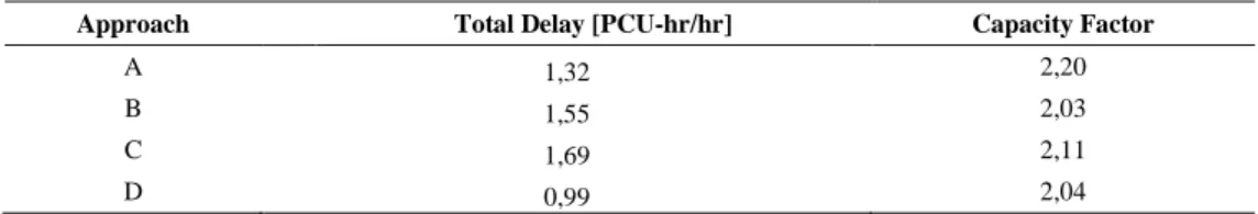
Numerical results are shown in Table 4.2 in which each row shows stage durations obtained with one of the objective functions described above, together with values of the other objective functions; best values are in bold. Population size values, the crossover probability/ rate (PC), and the mutation probability/ rate (PM) are given in the table.

Table 4.2 -Results of monocriteria SSD - Population size = 40.

At first it can be observed that values of stage durations are affected by the criterion considered as objective functions; by comparing obtained results the best value of each indicator is consistent with the optimisation criterion (i.e. in case of CF optimisation, CF = 1.35 and this is the best value of CF among all).

Furthermore, about other indicators, in case of TD minimisation lower value of TD is obtained (TD=9.14 veh); in case of CF maximisation, higher value of capacity factor is reached (CF=1.35); finally, in case of NS minimisation lower value of NS is obtained (NS=397.88 stops/h). Furthermore, the proposed approach was also

Criterion PC/PM TD (veh-h/h) CF NS (stops/h) t1(s) t2(s) t3(s)

TD 0.8/0.001 9.14 1.32 459.76 28 20 16 CF 0.9/0.0001 9.15 1.35 459.76 28 20 16 Nvq 0.9/0.0001 12.01 1.16 397.87 23 18 23

validated by comparing GAs results with SIGCAP and SIGSET results. Starting from monocriteria SSD results, multicriteria SSD problem was investigated preliminary assessing the speed of convergence with respect to parameter values (i.e. population size and PC, PM pairs). The GPR and the NSGA-II methods were performed and results are shown in Table 4.3.

Table 4.3 -Results of multicriteria SSD (GPR; NSGA-II); Population size = 40.

*C=criterion considered in the objective function

In particular, three kinds of evaluations can be made: (i) with respect to the effectiveness of each multicriteria optimisation, results obtained by combining TD and CF are better than results obtained by combining TD and NS; (ii) with respect to the comparison between NSGA-II and GPR, more satisfactory results can be obtained by the application of the first one in particular with regard to TD and CF; (iii) finally, with respect to the comparison between monocriteria (based on CF) and multicriteria methods (based on TD&CF), no significant differences can be

appreciated between the first one (TDmono= 9.15 veh; CFmono=1.35; NSmono=459.76

stops/h) and the second one (TD&CF: TDmulti= 9.23 veh; CFmulti=1.33;

NSmulti=450.92 stops/h); however CF and TD were better in case of monocriteria

optimisation than multicriteria optimisation, while a lower (and better) value of total number of stops can be appreciated in case of NSGA- II than monocriteria optimisation.

4.6 Conclusions and research perspectives

This paper is addressed to preliminary investigate the GAs application to the monocriteria or multicriteria SSD for a single junction.

In case of monocriteria optimisation three criteria were considered based on total delay minimisation, capacity factor maximisation and total number of stops minimisation. Monocriteria GAs based on CF maximisation and TD minimisation were compared to SIGCAP and SIGSET methods in order to consolidate their effectiveness of the method. In case of multicriteria optimisation the combination of total delay minimisation and capacity factor maximisation and the combination of total delay minimisation and total number of stops minimisation were considered.

Two algorithms were compared: the GPR and the NSGA-II. On the base of obtained results it can be observed that NSGA-II outperforms GPR. Furthermore, monocriteria GAs were compared to multicriteria GAs (in particular with NSGA-II method). Results show that no significant differences can be appreciated with respect to the values of indicators (TDmono=9.14 veh; CFmono=1.35 vs. TDmulti=9.23

Opt. Meth. C*1 C*2 PC/PM TD (veh-h/h) CF NS (stops/h) t1(s) t2(s) t3(s) GPR TD CF 0.9/0.0001 9.45 1.26 450.93 26 21 17 NS 0.8/0.001 10.35 1.17 442.08 29 17 18 NSGA-II TD CF 0.9/0.0001 9.23 1.33 450.92 27 20 17 NS 0.8/0.001 10.18 1.23 468.60 31 18 15

veh; CFmulti=1.33) while better results of total number of stops are carried by the

application of multicriteria optimisation (NSmulti=450.92 stops/h) than monocriteria

optimisation (NSmono=459.76 stops/h).

In future papers, procedures with cycles length optimisation will be addressed. Furthermore obtained results will be compared to other metaheuristics (such as the Simulated Annealing). In particular, the interest in further investigations about application of other metaheuristics to SSD, is related to the complexity of GAs implementation; in fact in this case an high number of parameters (such as crossover rate, mutation rate, population size) must be set preliminarily.

Finally, the integration of multicriteria SSD within the traffic assignment problem with variable demand (see [10]) will be investigated.

References

[1]Akcelik, R. (1981). Traffic Signals: Capacity and Timing Analysis. Research Report ARR No.123. ARRB Transport Research Ltd, Vermont South, Australia.

[2]Allsop, R., E. (1971a). Delay minimising settings for fixed time traffic signals at a single junction. Journal of the Institute of Mathematics and its Applications, 164-185.

[3]Allsop, R., E. (1972). Estimating the traffic capacity of a signalized road junction. Transportation Research, 245-255.

[4]Baker, J.E. (1985). Adaptive selection methods for genetic algorithms. Proceedings of the 3rd International Conference on Genetic Algorithms and Applications, In: Grefenstette, J.J. (ed.), New Jersey, Lawrence Erlbaum: Hillsdale, 100-111.

[5]Benekohal, R.F., Waller, S. T. (2003). Multiobjective traffic signal timing optimization using non-dominated sorting genetic algorithm. In Intelligent Vehicle Symposium, Proceedings IEEE 9, 198 – 203.

[6]Cantarella, G., E., Improta, G. (1983). A nonlinear model for control system design at an individual signalized junction. Operation Research Italian Society proceedings of the Conference, 709-722.

[7]Cantarella, G., E., Improta, G. (1988). Capacity Factor or Cycle Time Optimization for Signalized Junctions: A Graph Theory Approach. Transportation Research B.

[8]Cantarella, G.E.; Di Pace, R.; Memoli, S.; de Luca, S. (2013a). The Network Signal Setting Problem: The Coordination Approach vs. the Synchronisation Approach. Computer Modelling and Simulation (UKSim), 2013 UKSim 15th International Conference, 575-579, doi: 10.1109/UKSim.2013.99.

[9]Cantarella, G.E.; Di Pace, R.; Memoli, S.; de Luca, S. (2013b). The Application of Multicriteria Genetic Algorithms for Signal Setting Design at a Single junction 8th EUROSIM Congress on Modelling and Simulation, 2013, 472-477, doi 10.1109/Eurosim.2013.85

[10]Cantarella, G.E., de Luca, S., Di Gangi, M. & Di Pace, R. (2013c). Stochastic equilibrium assignment with variable demand: Literature review, comparisons and research needs. WIT Transactions on the Built Environment, Vol. 130, 349-364

[11]Ceylan, H., Bell, MGH (2005). Genetic algorithm solution for the stochastic equilibrium transportation networks under congestion. Transportation Research Part B, 39, 169–185. [12]Deb, k., Pratap, A., Agarwal, S., Meyarivan, T. (2002) A Fast and Elitist Multiobjective Genetic

Algorithm:NSGA-II. IEEE Transactions on Evolutionary Computation, vol. 6, NO. 2, 182-197. [13]Foy, M. D., Benekohal, R. F. and Goldberg, D. E. (1992). Signal Timing Determination using

genetic algorithms. Transportation Research Record 1365, 108-115.

[14]Gallivan , S., Heydecker, B., G. (1988). Optimising the control performance of traffic signals at a single junction. Transportation Research B, 357-370.

[15]Gazis, D., C. (1964). Optimal control of a system of oversaturated intersections. Operations Research, 815-831.

[16]Girianna, M. and Benekohal, R. F. (2004). Using Genetic Algorithms to design signal coordination for oversaturated networks. Intelligent Transportation Systems, 8, 117-129 [17]Goldberg, D.E. (1989).Genetic Algorithms in Search, Optimization, and Machine Learning.

Addison-Wesley, Reading, MA

[18]Holland, J.H. (1975). Adaptation in Natural and Artificial System. The University of Michigan Press.

[19]Improta, G., Cantarella, G.E. (1984). Control system design for an individual signalized junction, Transportation Research B, 147-168

[20]Michalopoulos, P., Stephanopolos, G. (1977). Oversaturated signal system with queue length constraints. Transportation Research, 413-421.

[21]Park, B., Messer, C. J. and Urbanik II, T. (1999). Traffic Signal Optimization Program for Oversaturated Conditions: Genetic Algorithms Approach. Transportation Research Record 1683, 133-142

[22]Putha, R., Quadrifoglio, L. and Zechman (2012). Comparing Ant Colony Optimization and Genetic Algorithm Approaches for Solving Traffic Signal Coordination under Oversaturation Conditions. Computer-Aided Civil and Infrastructure Engineering, 27, 14–28.

[23]Renfrew, D., Xiao-Hua Yu (2012). Traffic Signal Optimization Using Ant Colony Algorithm. IEEE, Brisbane, Australia, 1-7.

[24]Sun, D., Benekohal, R.F., Waller, S. T. (2003a). Multiobjective traffic signal timing optimization using non-dominated sorting genetic algorithm in Intelligent Vehicle Symposium, Proceedings IEEE 9, 198 – 203.

[25]Sun, D., Benekohal, R.F., Waller, S. T. (2003b). Bi-level Programming Formulation and Heuristic Solution Approach for Dynamic Traffic Signal Optimization. Computer-Aided Civil and Infrastructure Engineering, 21, 321–333

[26]Teklu F., Sumalee A., Watling D.P. (2007). A genetic algorithm approach for optimising traffic control signals considering routing. Journal of Computer-Aided Civil and Infrastructure Engineering, 22, 31-43.

[27]Webster, F. V. (1958). Traffic Signal Settings. Road Research Technical Paper, 39, HMSO, London.