A DEA MEASURE FOR MUTUAL FUNDS PERFORMANCE
Antonella Basso
Dep. of Applied Mathematics “B. de Finetti”, University of Trieste Stefania Funari
Dep. of Applied Mathematics, University Ca’ Foscari of Venice
Abstract: In this paper we propose a data envelopment analysis (DEA) approach in order to evaluate the efficiency of mutual funds. Our DEA performance index for mutual funds generalizes many well known traditional indexes and allows to take into account many conflicting objectives (the expected return and different risk measures), together with the investment costs (subscription costs and redemption fees). Moreover the use of the DEA methodology allows to identify, for each mutual fund, a composite portfolio which can be considered as a personalized benchmark. The DEA performance measure has been tested on the Italian financial market and the results are compared with the ranking obtained with some traditional performance indexes. Keywords: mutual funds performance, data envelopment analysis, fractional programming, linear programming.
1. Introduction
The data envelopment analysis (DEA) is an optimization based technique that has been proposed by Charnes, Cooper and Rhodes [5] to measure the relative efficiency of public sector activities and no profit organizations, such as for example educational institutions and health services.
The DEA efficiency measure is computed by solving a fractional linear programming model that can be converted into an equivalent linear programming problem which can be easily solved.
Afterwards, the same methodology has been applied to many profit oriented companies, such as bank branches. For a review of various applications, see for example Seiford [11].
The main purpose of this contribution is to use the DEA methodology in order to compute a mutual fund performance index that can take into account many conflicting objectives together with the costs required by the investment. In particular, the traditional performance indexes proposed in the literature do not allow to consider investment costs such as the subscription and redemption costs, while the DEA
approach can naturally include many costs among the inputs of the model.
On one hand the DEA performance index for mutual funds can be considered as a generalization of many traditional ratios such as Sharpe, Treynor, and reward to half-variance ratios. On the other hand the DEA methodology may be used as a multi-criteria decision method to evaluate the performance of mutual funds.
In addition, the results of the DEA technique can be used in order to identify, for each inefficient decision making unit, a corresponding efficient set (called peer group) which represents a “virtual” composite portfolio. This composite portfolio can be seen as a personalized benchmark and characterizes the portfolio style.
The structure of the paper is as follows. In Section 2 we briefly describe the data envelopment analysis approach and focus in particular on the input-oriented CCR model. In Section 3 we introduce the DEA performance index of mutual fund investments, whereas in Section 4 we describe how to build composite portfolios to be used as benchmarks. In Section 5 the DEA performance index is tested on the Italian financial market. Finally, some concluding remarks and suggestions for future research are presented in Section 6.
2. The data envelopment analysis
The data envelopment analysis (DEA) is an optimization based technique that allows to measure the relative performance of decision making units which are characterized by a multiple objectives and/or multiple inputs structure.
Operational units of this kind, for example, tipically include no profit and governmental units such as schools, hospitals, universities. In these units, the presence of a multiple output–multiple input situation makes difficult to identify an evident efficiency indicator such as profit and complicates the search for a satisfactory measure of efficiency.
Charnes, Cooper and Rhodes [5] proposes a measure of efficiency which is essentially defined as a ratio of weighted outputs to weighted inputs. In a sense, the weighted sums allow to reduce the multiple input–multiple output situation to a single “virtual” input–“virtual” output case; the efficiency measure is then taken as the ratio of the virtual output to the virtual input. Of course, the higher the efficiency ratio is, the more efficient the unit is.
Such a weighted ratio requires a set of weights to be defined and this can be not easy. Charnes, Cooper and Rhodes’s idea is to define the efficiency measure by assigning to each unit the most favourable weights. On the one hand, this means that the weights will generally not be the same for the different units. On the other hand, if a unit
turns out to be inefficient, compared to the other ones, when the most favourable weights are chosen, we cannot say that this depends on the choice of the weights!
The most favourable weights are chosen as the ones which maximize the efficiency ratio of the unit considered, subject to the constraints that the efficiency ratios of all units, computed with the same weights, have an upper bound of 1. Therefore, an efficiency measure equal to 1 characterizes the efficient units: at least with the most favourable weights, these units cannot be dominated by the other ones in the set. We obtain a Pareto efficiency measure in which the efficient units lie on the efficient frontier (see Charnes, Cooper, Lewin and Seiford [7]).
Let us define:
j = 1, 2, . . . , n decision making units r = 1, 2, . . . , t outputs
i = 1, 2, . . . , m inputs
yrj amount of output rfor unit j xij amount of input ifor unit j
ur weight given to output r
vi weight given to input i
The DEA efficiency measure for the decision making unit j0 (j0 = 1, 2, . . . , n) is computed by solving the following fractional linear programming model max {vi,ur} h0= ∑t r=1uryrj0 ∑m i=1vixij0 (2.1) subject to ∑ t r=1uryrj ∑m i=1vixij ≤ 1 j = 1, . . . , n ur≥ ϵ r = 1, . . . , t vi≥ ϵ i = 1, . . . , m (2.2)
whereϵis a convenient small positive number that prevents the weights be zero.
The above ratio form has an infinite number of optimal solutions: in fact, if (v1, . . . , vm, u1, . . . , ut) is optimal, then β(v1, . . . , vm, u1, . . . , ut) is also optimal for all β > 0. One can define an equivalence relation that partitions the set of feasible solutions of problem (2.1)-(2.2) into equivalence classes. Charnes and Cooper [4] and Charnes, Cooper Lewin and Seiford [7] propose to select a representative solution from each equivalence class. The representative solution that is usually chosen in DEA modelling is that for which ∑mi=1vixij0 = 1in the input-oriented forms and that with ∑tr=1uryij0 = 1 in the output-oriented models.
In this way the fractional problem (2.1)-(2.2) can be converted into an equivalent linear programming problem which can be easily solved. Using the input-oriented form we thus obtain the so called input-oriented CCR (Charnes, Cooper and Rhodes) linear model; its dual problem is also useful, both for computational convenience (as it has usually less constraints than the primal problem) and for its significance:
Input–oriented CCR primal model
max t ∑ r=1 uryrj0 subject to m ∑ i=1 vixij0= 1 t ∑ r=1 uryrj− m ∑ i=1 vixij ≤ 0 j = 1, . . . , n − ur≤ −ϵ r = 1, . . . , t − vi≤ −ϵ i = 1, . . . , m
Input–oriented CCR dual model
min z0− ϵ t ∑ r=1 s+r − ϵ m ∑ i=1 s−i subject to xij0z0− s−i − n ∑ j=1 xijλj= 0 i = 1, . . . , m − s+ r + n ∑ j=1 yrjλj= yrj0 r = 1, . . . , t λj≥ 0 j = 1, . . . , n s−i ≥ 0 i = 1, . . . , m s+r ≥ 0 r = 1, . . . , t z0 unconstrained
The CRR primal problem hast + mvariables (the weightsur andvi which have to be chosen so as to maximize the efficiency of the targeted unit j0) and n + t + m + 1constraints.
It can be seen that the CCR model gives a piecewise linear production surface which, in economic terms, represents a production frontier: in fact, it gives the maximum output empirically obtainable from a decision making unit given its level of inputs; from another point of view, it gives the minimum amount of input required to achieve the given output levels. The input-oriented models focus on the maximal movement toward the frontier through a reduction of inputs, whereas the output-oriented ones consider the maximal movement via an augmentation of outputs.
DEA model (2.1)-(2.2) is the first, simplest and still most used DEA technique. Nevertheless, in the meantime a number of extensions and variants have been proposed in the literature to better cope with special purposes; for a review see for example Charnes, Cooper, Lewin and Seiford [7]. Though born to evaluate the efficiency of no profit institutions, soon afterwards the DEA technique has been applied to measure the efficiency of any organizational unit; for example it has largely been used to compare the performance of different bank branches.
3. A DEA performance measure of mutual funds investments In order to completely rank a set of investment funds, some numerical indexes have been proposed in the literature that evaluate the performance of mutual funds by taking into account both expected return and risk and synthesizing them in a unique numerical value. Among these indexes we recall the reward to volatility ratio (Sharpe [12]), the reward to half-variance index and the reward to semivariance index (Ang and Chua [1]) and the reward to variability ratio (Treynor [14]). On the other hand, we have to point out that these indicators do allow to compare any couple of portfolios, by suggesting to choose the one with the higher index value, but are based on strong assumptions on the market behaviour and investors’ preferences. Other techniques that have been introduced to evaluate the performance of mutual funds refer to multi-criteria decision making methods; these approaches recognize the existence of a trade-off between conflicting objectives such as the portfolio expected return and its risk.
We have seen in Section 2 that DEA takes into account a multiple input-multiple output situation by computing a performance measure that is based on the virtual output/input ratio. Let us partition the conflicting objectives of a multi-criteria problem into two groups: an output set which includes the desirable objectives (those to be maximized) and an input set including the undesirable ones (those to be minimized). Then the DEA methodology may be used, in some sense,
as a multi-criteria approach in which the weights that allow to aggregate the objectives are not fixed in advance in a subjective manner but are determined as the most favourable weights for each unit (and may be different for the various units). On this subject refer to Joro, Korhonen and Wallenius [9] which makes a direct comparison between DEA and multiple objective linear programming models.
Our idea is to use the DEA methodology in order to compute a mutual fund performance index that can take into account many conflicting objectives together with the costs required by the investment. In effect, we can assign the desirable objectives, such as the return, to the output set and the undesirable objectives to the input set. For example, all the possible risk measures, such as standard deviation or half-variance, together with subscription costs and redemption fees, may be included among the inputs as undesirable objective to be minimized. By applying the DEA approach with these definitions, we obtain a performance measure that generalizes many of the traditional performance indicators, such as the reward to volatility ratio (Sharpe [12]), the reward to half-variance index (Ang and Chua [1]) and the reward to variability ratio (Treynor [14]). These indexes are ratios between the expected excess return (an output) and a different risk indicator (an input)
ISharpe= E(R)− r σR , Ihalf−var= E(R)− r HVR , IT reynor = E(R)− r β
where (E(R)− r)denotes the expected excess return, i.e. the difference between the portfolio expected return E(R) and the riskless rate of return r, σR =
√
V ar(R) is the standard deviation of the return, HVR denotes the half-variance risk indicator HVR = E (min [R− E(R), 0])
2 ; andβ represents the ratio of the covariance between the portfolio return R and the market portfolio return Rm to the variance V ar(Rm) of the market portfolio return i.e. β = Cov(R, Rm)/V ar(Rm).
On the contrary, the DEA efficiency measure is a ratio of a weighted sum of outputs (the portfolio return and eventually some other desirable objectives) to a weighted sum of inputs (one or more risk measures, the investment costs that the traditional indexes do not consider, and eventually some other undesirable features).
A first attempt to apply the DEA methodology in order to obtain a mutual funds efficiency indicator is the DPEI index developed by Murthi, Choi and Desai [10]. The DPEI index considers the mutual fund return as output and the standard deviation and transaction costs as inputs. Nevertheless, among the various transaction costs, it considers also operational expenses, management fees and purchase and sale costs incurred by the management, which are costs that have already been
deduced from the net return. On the contrary, we prefer to take into account subscription costs and redemption fees that directly burden the investors but not the expenses that have already been deduced from the net return of the portfolio.
As we have seen, the DEA approach allows to consider many outputs and many inputs. However, in this contribution we propose some performance measures that take into account only one output, the portfolio expected returnE(R), and many inputs. The inputs considered are a risk measure, (eventually) the β as a measure of risk which is relevant when the investor’s portfolio is well diversified and one or more subscription and redemption costs.
Let us consider a set ofnmutual funds with expected returnE(Rj), j = 1, 2 . . . , n, and denote, as before, the levels of the m inputs of fund j by xij, i = 1, 2, . . . , m. Let us compute the relative efficiency of fund j0. The DEA performance index of mutual fund investments that we propose, IDEA, is defined as the maximum value of the objective function, computed with respect to the output weight uand the input weights vi,i = 1, 2, . . . , m, of the following fractional linear problem
max {vi,u} I =∑uE(Rj0) m i=1vixij0 (3.1) subject to uE(Rj) ∑m i=1vixij ≤ 1, j = 1, . . . , n u≥ ϵ vi≥ ϵ i = 1, . . . , m (3.2)
Using the same device discussed in Section 2, the fractional problem (3.1)-(3.2) can be converted into an equivalent input-oriented linear model. The resulting primal and dual problems are as follows
Mutual funds primal model
max uE(Rj0) subject to m ∑ i=1 vixij0 = 1 uE(Rj)− m ∑ i=1 vixij ≤ 0 j = 1, . . . , n − u ≤ −ϵ − vi≤ −ϵ i = 1, . . . , m
Mutual funds dual model min z0− ϵs+− ϵ m ∑ i=1 s−i subject to xij0z0− s − i − n ∑ j=1 xijλj= 0 i = 1, . . . , m − s++ n ∑ j=1 E(Rj)λj= E(Rj0) λj≥ 0 j = 1, . . . , n s−i ≥ 0 i = 1, . . . , m s+≥ 0 z0 unconstrained.
By letting νi = vi/u, i = 1, 2, . . . , m, the mutual funds problems can be equivalently written in the following (output-oriented) reduced form
Reduced primal model
min m ∑ i=1 νi xij0 E(Rj0) subject to m ∑ i=1 νixij≥ E(Rj) j = 1, . . . , n νi≥ ε i = 1, . . . , m where εis a suitable small positive number.
Reduced dual model
max n ∑ j=1 λjE(Rj) + ε m ∑ i=1 s−i subject to n ∑ j=1 λjxij+ s−i = xij0 E(Rj0) i = 1, . . . , m λj ≥ 0 j = 1, . . . , n s−i ≥ 0 i = 1, . . . , m
4. Peer groups as benchmark portfolios
The measures of the relative efficiency of the decision making units represent only one kind of information resulting from the DEA methodology. An important feature of the DEA approach is its ability not only to verify if a decision making unit is efficient, relative to the other units, but also to suggest to the inefficient units a “virtual unit” that they could imitate in order to improve their efficiency.
In fact, for each inefficient unit the solution of the input-oriented CCR dual model presented in Section 2 permits to identify a set of corresponding efficient units, called peer units, which are efficient with the inefficient unit’s weights. The peer units are associated with the (strictly) positive basic multipliersλi, that is the non null dual variables. Therefore, for each inefficient unit j0 it is possible to build a composite unit with output
n ∑ j=1 λjyrj r = 1, . . . , t (4.1) and input n ∑ j=1 λjxij i = 1, . . . , m (4.2)
that outperforms unit j0 and lies on the efficient frontier.
From a financial point of view, this composite unit can be considered as a benchmark for the inefficient fund j0. Fund j0 could improve its performance by trying to imitate the behaviour of the efficient composite unit, i.e. of its benchmark portfolio. This (efficient) benchmark portfolio has an input/output orientation or style which is similar to that of the (inefficient) fundj0.
Therefore, the benchmark composite unit can be useful in studying the style of the portfolio management, and the importance of analyzing the management style of an asset portfolio is now well recognized in finance (see Sharpe [13]).
Since the output that we consider in the DEA model is the expected return, the different mutual funds (units) are scaled in terms of the same amount of invested capital. For this reason it can be interesting to compute the normalized multipliers
λj = λj
∑n k=1λk
(4.3)
5. An empirical analysis
We have tested the DEA performance index of mutual fund investments proposed in Section 3 on the Italian financial market. We have considered the weekly logarithmic returns of 47 mutual funds, for which homogeneous information are available, and of the Milan stock exchange Mibtel index (closing price). We have also considered, in some experiments, the instantaneous rate of return of the 12 months B.O.T. measured on a weekly base. The data regard the Monday net prices in the period 1/1/1997 to 31/12/1998 (104 weeks).
The mutual funds have been chosen from different classes (using the Assogestioni classing valid in the period considered: Az denotes a stocks fund, Bi a balanced fund and Ob a bonds one), with different total capital and from different management companies.
As noted in the previous section, we consider as unique output the portfolio expected return. It is worth noting that we prefer to use the expected return as output instead of the excess return, as would be suggested by a direct generalization of the Sharpe index, in order to limit the presence of negative values among the outputs. Just to allow the comparison with the riskless rate of return, we have included in some experiments a B.O.T. among the funds to be compared.
Among the inputs, we have considered a risk measure; this has been chosen either as the portfolio standard deviation σR or as the square root of the half-variance HVR. Moreover, in some analysis we have also included the β coefficient as an additional measure of risk which is relevant when the investor’s portfolio is well diversified; the market portfolio has been taken as the Mibtel index. In addition, we have considered the per cent subscription costs per different amounts of initial investment (10, 50 and 100 millions of Italian lire) and the per cent redemption costs per year of disinvestment (after 1, 2 or 3 years). Table 1 shows the results obtained with the DEA approach by comparing the stocks, balanced and bonds mutual funds separately, using standard deviation as a risk measure. In column 3 (3 inputs) the inputs include standard deviation, a subscription and a redemption cost while columns 4 and 5 report the DEA performance measures when the inputs include standard deviation and all the subscription and redemption costs (7 inputs); the symbol(+B) indicates the columns in which a B.O.T is added to the reference set.
From this table one of the most powerful features of the DEA performance measure becomes evident, i.e. the possibility to take into account also the investment costs that the other traditional criteria have to neglect. This explains the different ranking of the mutual funds obtained with DEA. Of course, including three levels of subscription
Table 1. DEA performance measures for the different classes of funds. The relative ranking is given in brackets.
Funds Classes 3 inputs(+B) 7 inputs(+B) 7 inputs
Stocks funds
Arca 27 Az2 0.562 (7) 0.562 (7) 0.562 (21)
Azimut Borse Int. Az2 0.295 (16) 0.313 (19) 0.545 (22)
Centrale Global Az2 0.187 (23) 0.242 (22) 0.591 (18)
EptaInternational Az2 0.343 (13) 0.389 (14) 0.717 (12)
Fideuram Azione Az2 0.158 (24) 0.233 (23) 0.544 (23)
Fondicri Int. Az2 0.220 (19) 0.320 (18) 0.584 (19)
Genercomit Int. Az2 0.218 (20) 0.329 (17) 0.668 (14)
Investire Intern. Az2 0.580 (6) 0.580 (6) 0.580 (20)
Prime Global Az2 0.335 (14) 0.382 (15) 0.652 (15)
Sanpaolo H. Intern. Az2 0.195 (22) 0.232 (24) 0.539 (24)
Centrale Italia Az3 0.353 (12) 0.442 (11) 0.903 (3)
Epta Azioni Italia Az3 0.495 (8) 0.549 (8) 0.868 (7)
Fondicri Sel. Italia Az3 0.373 (10) 0.534 (9) 0.938 (2)
Genercomit Azioni It. Az3 0.874 (2) 0.874 (2) 0.874 (6)
Gesticredit Borsit Az3 0.392 (9) 0.520 (10) 0.893 (4)
Imi Italy Az3 0.287 (17) 0.370 (16) 0.881 (5)
Investire Azion. Az3 0.847 (3) 0.847 (3) 0.847 (8)
Oasi Azionario Itali Az3 1.000 (1) 1.000 (1) 1.000 (1)
Azimut Europa Az4 0.372 (11) 0.393 (13) 0.651 (16)
Gesticredit Euro Az. Az4 0.330 (15) 0.398 (12) 0.742 (11)
Imi Europe Az4 0.199 (21) 0.262 (21) 0.716 (13)
Investire Europa Az4 0.790 (4) 0.790 (4) 0.790 (10)
Sanpaolo H. Europe Az4 0.229 (18) 0.272 (20) 0.629 (17)
Indice Mibtel 0.667 (5) 0.681 (5) 0.821 (9)
B.O.T. 1.000 (1) 1.000 (1)
Balanced funds
Arca BB Bi1 1.000 (1) 1.000 (1) 1.000 (1)
Azimut Bil. Bi1 0.401 (6) 0.431 (8) 0.915 (5)
Eptacapital Bi1 0.390 (7) 0.449 (6) 0.924 (4)
Genercomit Bi1 0.287 (8) 0.445 (7) 0.996 (3)
Investire Bil. Bi1 0.996 (2) 0.996 (2) 0.996 (2)
Arca TE Bi2 0.702 (3) 0.702 (3) 0.702 (7)
Fideuram Performance Bi2 0.683 (4) 0.683 (4) 0.683 (8)
Fondo Centrale Bi2 0.123 (10) 0.169 (10) 0.458 (10)
Genercomit Espansion Bi2 0.189 (9) 0.296 (9) 0.682 (9)
Indice Mibtel 0.631 (5) 0.644 (5) 0.766 (6)
B.O.T. 1.000 (1) 1.000 (1)
Bonds funds
Arca Bond Ob3 0.311 (4) 0.311 (5) 0.311 (8)
Azimut Rend. Int. Ob3 0.095 (14) 0.099 (14) 0.143 (14)
Epta 92 Ob3 0.129 (11) 0.147 (12) 0.275 (10)
Genercomit Obb. Este Ob3 0.334 (3) 0.339 (4) 0.339 (7)
Imi Bond Ob3 0.128 (12) 0.172 (11) 0.395 (6)
Investire Bond Ob3 0.238 (7) 0.241 (9) 0.241 (13)
Oasi Bond Risk Ob3 0.254 (6) 0.254 (8) 0.254 (12)
Primebond Ob3 0.182 (9) 0.226 (10) 0.299 (9)
Sanpaolo H. Bonds Ob3 0.098 (13) 0.116 (13) 0.256 (11)
Bpb Tiepolo Ob5 1.000 (1) 1.000 (1) 1.000 (1)
Centrale Tasso Fisso Ob5 0.215 (8) 0.269 (6) 0.545 (4)
Eptabond Ob5 0.283 (5) 0.371 (3) 0.657 (2)
Fideuram Security Ob5 1.000 (1) 1.000 (1) 1.000 (1)
Oasi Btp Risk Ob5 0.589 (2) 0.589 (2) 0.589 (3)
Prime Reddito Italia Ob5 0.180 (10) 0.267 (7) 0.519 (5)
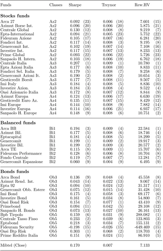
Table 2. Values of Sharpe, Treynor and reward to half-variance indexes. The relative ranking is given in brackets.
Funds Classes Sharpe Treynor Rew.HV
Stocks funds
Arca 27 Az2 0.092 (23) 0.006 (18) 7.601 (15)
Azimut Borse Int. Az2 0.096 (20) 0.006 (20) 5.875 (21)
Centrale Global Az2 0.130 (12) 0.008 (8) 9.219 (7)
Epta-International Az2 0.094 (21) 0.005 (23) 5.752 (22)
Fideuram Azione Az2 0.105 (17) 0.007 (16) 6.281 (20)
Fondicri Int. Az2 0.117 (14) 0.008 (3) 9.195 (8)
Genercomit Int. Az2 0.102 (19) 0.007 (14) 7.108 (16)
Investire Int. Az2 0.117 (15) 0.007 (13) 8.233 (13)
Prime Global Az2 0.093 (22) 0.006 (22) 5.726 (23)
Sanpaolo H. Intern. Az2 0.103 (18) 0.006 (19) 6.762 (18)
Centrale Italia Az3 0.207 (1) 0.009 (1) 10.780 (1)
Epta Azioni Italia Az3 0.177 (6) 0.008 (10) 8.833 (11)
Fondicri Sel. Italia Az3 0.179 (5) 0.008 (7) 9.258 (6)
Genercomit Azioni It. Az3 0.190 (2) 0.008 (2) 10.654 (3)
Gesticredit Borsit Az3 0.177 (7) 0.008 (11) 9.507 (5)
Imi Italy Az3 0.184 (4) 0.008 (5) 8.836 (10)
Investire Azion. Az3 0.184 (3) 0.008 (4) 9.522 (4)
Oasi Azionario Italia Az3 0.172 (8) 0.007 (12) 8.844 (9)
Azimut Europa Az4 0.124 (13) 0.006 (17) 6.630 (19)
Gesticredit Euro Az. Az4 0.135 (11) 0.007 (15) 8.429 (12)
Imi Europe Az4 0.144 (10) 0.008 (9) 7.882 (14)
Investire Europa Az4 0.114 (16) 0.006 (21) 6.937 (17)
Sanpaolo H. Europe Az4 0.148 (9) 0.008 (6) 10.751 (2)
Balanced funds
Arca BB Bi1 0.194 (3) 0.009 (4) 22.584 (1)
Azimut Bil. Bi1 0.177 (5) 0.008 (6) 18.746 (4)
Eptacapital Bi1 0.181 (4) 0.008 (5) 18.299 (5)
Genercomit Bi1 0.199 (1) 0.009 (2) 19.917 (3)
Investire Bil. Bi1 0.199 (2) 0.009 (3) 20.577 (2)
Arca TE Bi2 0.115 (8) 0.009 (1) 15.707 (6)
Fideuram Performance Bi2 0.128 (6) 0.006 (8) 10.704 (8)
Fondo Centrale Bi2 0.119 (7) 0.007 (7) 12.281 (7)
Genercomit Espansione Bi2 0.060 (9) 0.004 (9) 6.495 (9)
Bonds funds
Arca Bond Ob3 0.136 (9) 0.048 (4) 45.558 (8)
Azimut Rend. Int. Ob3 0.043 (14) 0.022 (13) 9.067 (14)
Epta 92 Ob3 0.094 (10) 0.024 (12) 31.317 (11)
Genercomit Obb. Estere Ob3 0.075 (12) 0.015 (14) 31.428 (10)
Imi Bond Ob3 0.175 (4) 0.058 (3) 69.177 (6)
Investire Bond Ob3 0.161 (5) 0.034 (8) 54.800 (7)
Oasi Bond Risk Ob3 0.154 (7) 0.077 (1) 43.410 (9)
Primebond Ob3 0.094 (11) 0.042 (5) 29.108 (12)
Sanpaolo H. Bonds Ob3 0.073 (13) 0.027 (10) 26.161 (13)
Bpb Tiepolo Ob5 0.159 (6) 0.031 (9) 288.082 (1)
Centrale Tasso Fisso Ob5 0.233 (2) 0.039 (6) 123.803 (3)
Eptabond Ob5 0.218 (3) 0.034 (7) 155.131 (2)
Fideuram Security Ob5 -0.198 (15) -0.026 (15) -649.469 (15)
Oasi Btp Risk Ob5 0.303 (1) 0.068 (2) 118.703 (4)
Prime Reddito Italia Ob5 0.151 (8) 0.024 (11) 86.910 (5)
Table 3. Peer groups and relative composition of the benchmark portfolios for the different classes of stocks funds in the model with 7 inputs (standard deviation and all the subscription and redemption costs). In column 2 a B.O.T. has been included in the reference set, too.
Stocks funds standardized multipliers(+B) standardized multipliers
Az2
1. Arca 27 efficient λ1=1.000 efficient λ1=1.000
2. Azimut Borse Int. λ1=0.171 λ12=0.829 λ1=0.234 λ4=0.766
3. Centrale Global λ1=0.092 λ12=0.908 λ4=1.000
4. EptaInternational λ1=0.153 λ12=0.847 efficient λ4=1.000
5. Fideuram Azione λ1=0.100 λ12=0.900 λ4=1.000
6. Fondicri Int. λ1=0.155 λ12=0.845 λ1=0.018 λ4=0.982
7. Genercomit Int. λ1=0.127 λ12=0.873 λ4=1.000
8. Investire Intern. efficient λ8=1.000 efficient λ8=1.000
9. Prime Global λ1=0.177 λ12=0.823 λ1=0.166 λ4=0.834
10. Sanpaolo H. Intern. λ1=0.101 λ12=0.899 λ4=1.000
11. Mibtel index efficient λ11=1.000 efficient λ11=1.000
12. B.O.T. efficient λ12=1.000
Az3
1. Centrale Italia λ8=0.086 λ10=0.914 λ8=1.000
2. Epta Azioni Italia λ8=0.147 λ10=0.853 λ8=1.000
3. Fondicri Sel. Italia λ8=0.166 λ10=0.884 λ8=1.000
4. Genercomit Azioni It. λ8=1.000 λ8=1.000
5. Gesticredit Borsit λ8=0.122 λ10=0.878 λ8=1.000
6. Imi Italy λ8=0.065 λ10=0.935 λ8=1.000
7. Investire Azion. λ8=1.000 λ8=1.000
8. Oasi Azionario Italia efficient λ8=1.000 efficient λ8=1.000
9. Mibtel index λ8=0.333 λ10=0.667 λ8=1.000
10. B.O.T. efficient λ10=1.000
Az4
1. Azimut Europa λ7=1.000 efficient λ1=1.000
2. Gesticredit Euro Az. λ7=1.000 efficient λ2=1.000
3. Imi Europe λ7=1.000 λ2=1.000
4. Investire Europa efficient λ4=1.000 efficient λ4=1.000
5. Sanpaolo H. Europe λ7=1.000 λ2=1.000
6. Mibtel index efficient λ6=1.000 efficient λ6=1.000
and redemption costs (linked to different amounts and durations of the investments) we emphasize the role of costs in the choice of the more efficient fund.
We observe that the inclusion of a B.O.T. in the reference set can be meaningful when the aim of the analysis is to offer investors a tool which help in choosing a convenient investment; on the other hand, if the analysis has the scope of evaluating the relative performance of the mutual funds management, then the reference set should includes only comparable funds. By comparing columns 4 and 5 of table 1 we notice that the exclusion of the B.O.T. from the reference set changes the relative ranking substantially, even if the efficient funds remain unchanged.
In order to compare the results obtained with the DEA approach, table 2 reports the values of Sharpe, Treynor and reward to half-variance indexes, with the associated ranking in brackets.
It has to be noticed that, contrary to the traditional indexes, the value of which don’t change when the set of mutual funds to be compared is modified, the DEA performance index does change its value according to the funds included in the reference set. Therefore, it may be interesting to see if the ranking of the funds in a class changes when we enlarge the reference set joining other classes of mutual funds. In Basso and Funari [2] it has been noted that the (relative) ranking inside each class is substantially preserved. What changes is the absolute value of the performance index and the fact that when we reduce the set of alternatives the fund with the highest efficiency measure becomes relatively efficient even if in the largest set it was not the most efficient one.
Moreover, it may be interesting to see if the choice of the risk measure considered among the inputs affects the funds ranking. An empirical analysis carried out in Basso and Funari [2] shows that considering standard deviations of the returns or the square root of the half-variance gives nearly the same results: this could means either that for the data under consideration these two risk measures are coherent or that the returns in the period chosen for this analysis are approximately symmetric. Furthermore, adding the β coefficient to the input set does not substantially modify the results, either, at least for the data under consideration.
Table 3 reports the peer groups and the relative composition of the benchmark composite portfolios for the different classes of stocks funds in the model with 7 inputs (standard deviation and all the subscription and redemption costs). We may observe that the efficient funds have no need to define a benchmark portfolio while they often enter in the benchmark portfolios of the other funds. Moreover, the inclusion in the reference set of the riskless asset modifies both the peer units and the
relative composition of the benchmark portfolios.
From table 3 we may also point out a feature of the DEA approach that has to be carefully considered when choosing the input set. In fact, the efficient units depend on the inputs that are chosen; therefore, the inclusion of inputs of minor importance should be avoided as they could make a fund become efficient on the ground of minor aspects.
By including the subscriptions and redemption costs we get efficiency results in which the role of low investment costs is emphasized. For example, in the Az2 fund, Arca 27 is efficient though neither its expected return is the highest one nor its standard deviation is the lowest one and the reason is probably due to the fact that it does not have any subscription and redemption cost. What’s more, the B.O.T. (which has low investment costs) is always efficient and is often included in the peer groups of the other mutual funds.
6. Concluding remarks
In this paper we propose to use the DEA methodology in order to evaluate the relative efficiency of mutual funds. The DEA performance index for mutual funds represents a generalization of many traditional numerical indexes and permits to take into account many conflicting objectives as well as the investment costs.
Moreover, the results of the DEA technique allow to identify, for each inefficient fund, a corresponding efficient set which represents a “virtual” composite portfolio. Such a peer group can be seen as a personalized benchmark and characterizes the portfolio style.
Some results obtained by testing the DEA performance index on the Italian financial market indicate the importance of the subscription and redemption costs in determining the fund ranking.
The results suggest that the DEA methodology for evaluating the mutual funds performance may usefully complement the traditional indexes. The DEA approach, indeed, provides some additional information that may be useful in carrying out a careful comparative analysis.
The DEA index we have proposed in this contribution considers many inputs but only one output, the portfolio expected return. A natural extension let to future research might take into account also a multiple output structure.
REFERENCES
[1] J.S. Ang and J.H. Chua, “Composite measures for the evaluation of investment performance”, Journal of Financial and Quantitative Analysis, Vol. 14, 1979, 361–384.
[2] A. Basso and S. Funari, “A data envelopment analysis approach to evaluate the performance of mutual funds”, Atti della giornata di studio su Metodi numerici per la finanza, Venezia, 7th May 1999.
[3] A. Boussofiane, R.G. Dyson and E. Thanassoulis , “Applied data envelopment analysis”, European Journal of Operational Research, Vol 52, 1991, 1–15.
[4] A. Charnes and W.W. Cooper, “Programming with linear fractional functionals”, Naval Res. Logist. Quart., Vol 9, 1962, 181–185.
[5] A. Charnes, W.W. Cooper and E. Rhodes, “Measuring the efficiency of decision making units”, European Journal of Operational Research, Vol 2, 1978, 429–444.
[6] A. Charnes, W.W. Cooper and E. Rhodes, “Short communication. Measuring the efficiency of decision making units”, European Journal of Operational Research, Vol 3, 1979, 339.
[7] A. Charnes, W.W. Cooper, A.Y. Lewin and L.M. Seiford, Data envelopment analysis: Theory, methodology, and application, Kluwer Academic Publishers, Boston, 1994.
[8] M.C. Jensen, “The performance of mutual funds in the period 1945– 1964”,Journal of Finance, Vol 23, 1968, 389–416.
[9] T. Joro, P. Korhonen and J. Wallenius, “Structural comparison of data envelopment analysis and multiple objective linear programming”, Management Science, Vol 44, 1998, 962–970.
[10] B.P.S. Murthi, Y.K. Choi and P. Desai, “Efficiency of mutual funds and portfolio performance measurement: A non-parametric approach”, European Journal of Operational Research, Vol 98, 1997, 408–418.
[11] L.M. Seiford, “Data envelopment analysis: The evolution of the state-of-the-art (1978–1995)”, Journal of Productivity Analysis, Vol 7, 1996, 99–138.
[12] W.F. Sharpe, “Mutual fund performance”, Journal of Business, Vol 34, 1966, 119–138.
[13] W.F. Sharpe, “Asset allocation: management style and performance measurement”, Journal of Portfolio Management, Vol 18, 1992, 7–19. [14] J.L. Treynor, “How to rate management of investment funds”, Harvard Business Review, January-March, 1965, 63–75.