Contents lists available atScienceDirect
Agricultural and Forest Meteorology
journal homepage:www.elsevier.com/locate/agrformetPhenology acts as a primary control of urban vegetation cooling and
warming: A synthetic analysis of global site observations
Yongxian Su
a,b, Liyang Liu
a,b, Jishan Liao
c⁎
, Jianping Wu
a
, Philippe Ciais
b, Jiayuan Liao
a,
Xiaolei He
a, Xiaodong Liu
d, Xiuzhi Chen
e,f,, Wenping Yuan
e,f, Guoyi Zhou
g, Raffaele Lafortezza
i,ha Key Lab of Guangdong for Utilization of Remote Sensing and Geographical Information System, Guangdong Open Laboratory of Geospatial Information Technology and
Application, Guangzhou Institute of Geography, Guangzhou 510070, China
b Laboratoire des Sciences du Climat et de l'Environnement, UMR 1572 CEA-CNRS UVSQ, 91191 Gif sur Yvette, France
c Department of Geography and City Planning, University of Toronto, Toronto, Ontario M5S 3G3, Canada
d College of Forestry and Landscape Architecture, South China Agricultural University, Guangzhou 510642, China
e Guangdong Province Key Laboratory for Climate Change and Natural Disaster Studies, School of Atmospheric Sciences, Sun Yat-sen University, Guangzhou 510275,
China
f Southern Marine Science and Engineering Guangdong Laboratory(Zhuhai), Zhuhai, China
g Institute of Ecology, Jiangsu Key Laboratory of Agricultural Meteorology, Nanjing University of Information Science & Technology, Nanjing 210044, China
h Department of Geography, The University of Hong Kong, Centennial Campus, Pokfulam Road, Hong Kong
i Department of Agricultural and Environmental Sciences, University of Bari “A. Moro”, Via Amendola 165/A, 70126 Bari, Italy
A R T I C L E I N F O Keywords:
Background climate Canopy shading
Cooling and warming effect Evapotranspiration Plant phenology Urban vegetation
A B S T R A C T
Urban vegetation can influence local air temperatures through its biophysical effects on surface energy balance. These effects produce gradients (ΔTa) between air temperature of vegetation spaces (Tveg) and air temperature of
open spaces (Topen) ( Ta=Tveg Topen), hereafter referred to as vegetation cooling (negative values of ΔTa) and
warming (positive values of ΔTa), respectively. But vegetation cooling or warming highly depends on
back-ground climate of urban areas as well as on vegetation states. Field observations are usually restricted to one or few cities, setting limitations to a general understanding. In this study, a synthetic analysis of 3634 point-scale in-situ observations from 77 global sites in 35 cites was conducted using the bootstrap sampling and hierarchical partitioning methods. Results show that vegetation cooling is generally stronger during the daytime periods, in warm seasons, at low latitude zones, for forest lands and at leaf growth stage, while vegetation warming usually occurs in the opposite contexts. Urban vegetation begins to exert considerable cooling effects when the daily mean background air temperature (BAT) is >10.0 °C, but on average has a slight warming effect when BAT is <10.0 °C. Besides, vegetation cooling increases sharply when evapotranspiration is >61.7 mm/month or when area of urban vegetation is >35.2 ha. Plant growth stages (i.e., canopy leaf growth, senescence and dormancy stages) (37.6 ± 0.11%), a vegetation phenology proxy, acts as the primary biotic factor, while seasonality (23.0 ± 0.11%) and latitude (11.4 ± 0.07%) that control the background climate are two most important abiotic contributors. Our findings suggest approximate thresholds for distinguishing vegetation cooling/ warming effects and provide helpful information for future urban greenspace planning aimed at mitigating local climate warming.
1. Introduction
Recently, there has been growing interest in mitigation of increased air temperature impacts on human health (Wolff et al., 2018; Su et al., 2019). Vegetation is commonly believed to considerably regulate local air temperatures (Ellison et al., 2017; Su et al., 2019). However, nearly 88% of global primary vegetation-covered land in urban areas has been destroyed and replaced by artificial surfaces in urbanization processes
during the past decades (Seto et al., 2012;d'Amour et al., 2016). This trend, in turn, has intensified urban climate warming locally (Sun et al., 2016). Additionally, more than 1.2 million km2of global lands have a
high probability (>75%) of being converted into urban areas by 2030 (Seto et al., 2012). Along with global climate warming, the local cli-mate in urban regions will increase in the future (Nakayama and Fujita, 2010;Escobedo et al., 2011;Oliveira et al., 2011).
Urban vegetation can influence local air temperature (Ta) through
https://doi.org/10.1016/j.agrformet.2019.107765
Received 24 May 2019; Received in revised form 17 September 2019; Accepted 19 September 2019
⁎Corresponding author.
E-mail address:[email protected](X. Chen).
0168-1923/ © 2019 Elsevier B.V. All rights reserved.
its effects on the surface energy balance (Cao et al., 2010a,b; Chen et al., 2012;Su et al., 2019), i.e., the so-called biophysical effect (Lee et al., 2011;Zeng et al., 2017), which is currently an active area of research with a myriad of practical applications (Oke, 1989; Bounoua et al., 2002;Georgi and Zafiriadis, 2006;Chang et al., 2007; Shashua-Bar et al., 2010; Oliveira et al., 2011; Susca et al., 2011; Chen et al., 2012). This effect produces gradients (ΔTa) between the air
temperature of vegetation spaces (Tveg) and air temperature of open
spaces (Topen) ( Ta=Tveg Topen), hereafter referred to as vegetation cooling and warming for negative and positive values of ΔTa,
respec-tively. The background climate in cities as well as vegetative functions have been investigated as two key forces for vegetation cooling and warming (Spronken-Smith and Oke, 1998; Su et al., 2019). The eva-porative cooling of vegetation (Taha et al., 1991; Dimoudi and Nikolopoulou, 2003;Jonsson, 2004;Bowler et al., 2010; Zhao et al., 2014; Feyisa et al., 2014), and shading of vegetation canopy which produces shade on understory spaces and regulates the incoming/out-going solar shortwave and infrared and longwave radiation (Oke, 1989; Pearlmutter et al., 1999; Dimoudi and Nikolopoulou, 2003; Bowler et al., 2010;Feyisa et al., 2014) are two most important func-tions inducing vegetation cooling. Low albedo of vegetation leads to a strong daytime radiative warming (Lee et al., 2011). Furthermore, ve-getation usually causes turbulence which brings heat from aloft to the near surface at nighttime and thereby generates nighttime warming (Lee et al., 2011). Background climate can influence the vegetation cooling and warming by controlling the directions of heat transfer (Zhang et al., 2013;Zhao et al., 2014;Li et al., 2015;Su et al., 2019), which changes the sensible heat fluxes and longwave radiation (Eq. (14), Zeng et al., 2017) and in turn the surface energy balance (Cao et al., 2010a,b;Chen et al., 2012;Su et al., 2019).
In contrast to satellite-based observations that record land surface temperatures (Ts) associated with surface energy budget (Bonan, 2008; Cao et al., 2010a,b;Lee et al., 2011;Peng et al., 2014; Zhang et al., 2014;Li et al., 2015; Alkama and Cescatti, 2016), field observations focus on Ta, which is a more reasonable climatic and environmental
indicator controlled by atmospheric mixing and used to characterize urban climate warming that requires closer attention (Su et al., 2019). Currently, the vegetation cooling and warming on local Tahas been
extensively studied worldwide using time-series field observations worldwide (Georgi and Zafiriadis, 2006; Potchter et al., 2006; Chang et al., 2007;Zhang et al., 2013;Su et al., 2019). For example, Dhakal and Hanaki (2002)reported that vegetation close to buildings lowers Ta maximally by 0.47 °C in Tokyo.Meier (1991) observed a
more enhanced cooling effect (ΔTa=−1.7 °C) of vegetation on Tain
California.Jauregui (1991)andWong and Yu (2005)detected a larger cooling magnitude of −3.0 °C to −4.0 °C in the tropical cities of Mexico and Singapore, from 1984 to 1987 and 1961 to 1963, respectively. Taha et al. (1991) also observed that urban vegetation produced a 6.0 °C lower Tathan in the surrounding environment during October of
1986 in Davis. A net warming of vegetation was also reported in some studies, e.g. Taipei (ΔTa=4.5 °C) (Chang et al., 2007) and Arava Valley
(ΔTa=2.2 °C) (Potchter et al., 2012). However, most field studies were
limited to one or few cities (Wong and Yu, 2005;Bowler et al., 2010; Feyisa et al., 2014), while at global scale the direction and magnitude of ΔTawere highly variable among cities (Georgi and Zafiriadis, 2006; Shashua-Bar et al., 2009;Su et al., 2019). A synthetic analysis to gen-eralize these point-scale results from global site observations is greatly warranted. In addition, uncertainty remains as to which of the under-lying factors control the background climate, evaporative cooling and canopy shading of vegetation in urban regions. Studies of cross-regional
Acronyms
Ta: air temperature; Ts: surface temperature;
Tveg: air temperature of vegetation spaces; Topen: air temperature of open spaces;
BAT: background air temperature of urban areas; ΔTa: published gradient between Tvegand Topen;
T*:a normalized gradient between Tvegand Topen;
∅: downward solar shortwave radiation (W m−2);
MAP: Mean annul precipitation (mm/year);
NDVI: Normalized Difference Vegetation Index;
EVI: Enhanced Vegetation Index;
LAI: Leaf Area Index;
PGS: Plant Growth Stage;
S: area of urban vegetation (ha);
ET: evapotranspiration (mm/month)
ETin situ: monthly ET calculated from in situ data (mm/month) ETMODIS: monthly ET extracted from MODIS products (mm/month)
Table 1 Data of global site in-situ observations. No. Longitude Latitude City Period Record Quantity Forest Type BAT (°C) MAP (mm) Average ΔT (°C) References 1 23.72 37.9 Athens 11,Jul,2005–31,Jul,2005 91 Tree block 36.13 1362.17 −2.14 Zoulia et al. (2009) 2 23.74 37.97 Oct, 2006–Jun,2007 45 Tree block 28.9 400 −0.12 Shashua-Bar et al. (2010) 3 116.39 39.37 Beijing Jun, 2006–Jul,2007 83 Tree block, Grass 31.1 483.9 −0.21 Liu et al. (2008) 4 116.42 39.87 Jun–Aug 37 Tree block, Grass 27.43 483.9 −3.41 Li et al. (1999) 5 116.33 39.93 Jul,2010 64 Tree block 35.68 630 −2.03 Yan et al. (2012) 6 116.27 39.97 11–20, Jul, 2010 10 Tree row 28.8 626 −0.62 Ji et al. (2012) 7 116.35 40 Aug–Oct, 2006 78 Tree row, Grass 21.1 731.7 −0.6 Ma and Li (2007) 8 116.37 40 11–20, Jul, 2010 5 Tree row 28.8 626 −0.82 Ji et al. (2012) 9 116.4 40 11–20, Jul, 2010 5 Tree row 28.8 626 −1.22 Ji et al. (2012) 10 116.4 40.02 11–20, Jul, 2010 5 Tree row 28.8 626 −1.18 Ji et al. (2012) 11 116.26 40.03 11–20,Jul,2010 5 Tree row 28.8 626 −0.84 Ji et al. (2012) 12 116.42 40.05 Jan–Oct,2011 100 − 20.55 483.9 −0.71 Ji et al. (2013) 13 116.09 40.06 29,Jul,2010–28,Mar,2011 192 Grass 26.88 630 −0.64 Wu et al. (2009) 14 116.35 40.25 11–20,Jul,2010 5 Tree row 28.8 626 −1.08 Ji et al. (2012) 15 116.4 40.58 11–20,Jul,2010 45 Tree block, Grass 31.8 626 −2.74 Zhu et al. (2011) 16 31.27 30.04 Cairo Jun, 2009 9 Tree block 41 26 −5.77 Mahmoud. (2011) 17 −121.76 38.54 Davis 12–18, Oct-1986 288 Tree block, Tree row 18.26 2000 −0.67 Taha et al. (1991) 18 112.99 28.13 Changsha Jan–Dec, 2005 120 Tree row 19.13 1780 −0.21 Luo (2013) 19 112.97 28.24 19–21,Jun,2007 14 Tree block, Tree row, Shrub 35.53 1422.4 −4.07 Zhao et al. (2007) 20 24.02 35.52 Chania-Crete 08–30, Jun, 2005 96 Tree block, Tree row 31.47 640 −3.05 Georgi and Dimitriou (2010) 21 106.62 29.58 Chongqing − 19 Tree block, Shrub, Grass 36 1200 −5.23 Feng et al. (2008) 22 35.24 30.66 En Yahav 1:00–22:00,07,Feb,2006 75 Tree block, Tree row, Grass 13.45 530.3 0.25 Potchter et al. (2012) 23 11.26 43.78 Florence 2002 24 Tree block − 679.99 −1.82 Bacci et al. (2003) 24 119.26 26.06 Fuzhou 07–09,Jul,2012 24 Tree block, Grass 38.13 1500 −1.37 Cai et al. (2013) 25 33.44 14.98 Gezira 19–27, Dec, 1964 43 Tree row 26.68 98 −1.9 Davenport and Hudson (1967) 26 11.47 57.7 Goteborg Apr–Jul, 1994 7 Tree block, Tree row −2.28 685.58 −4.38 Upmanis et al. (1998) 27 136.92 35.16 Goya Mar–Oct,2004 33 Tree block 10 560 −2.72 Cao et al. (2010a , b ) 28 136.98 35.17 Goya Aug,2006–Apr,2007 211 Tree row 28.86 1564.6 −0.85 Hamada and Ohta (2010) 29 113.74 23 Guangzhou 12:00, 17,Oct,2009; 1, Jun,2011 2 Tree block 27.65 1366.51 −1.91 Chen et al. (2012) 30 113.23 23.1 12:00, 06,Oct,2005 1 Tree block 33.5 1366.51 −2.94 Su et al. (2010) 31 113.28 23.1 12:00, 06,Oct,2005 1 Tree block 32.67 1366.51 −2.46 Su et al. (2010) 32 113.29 23.11 12:00, 06,Oct,2005 1 Tree block 32.93 1366.51 −4.24 Su et al. (2010) 33 113.23 23.12 12:00, 17,Oct,2009; 1, Jun,2011 2 Tree block 28.51 1366.51 −4.31 Chen et al. (2012) 34 113.34 23.12 12:00, 17,Oct,2009; 1, Jun,2011 2 Tree block 29.08 1366.51 −2.11 Chen et al. (2012) 35 113.23 23.13 12:00, 06,Oct,2005 1 Tree block 32.88 1366.51 −2.91 Su et al. (2010) 36 113.25 23.13 12:00, 17,Oct,2009; 1, Jun,2011 2 Tree block 29.54 1366.51 −3.49 Chen et al. (2012) 37 113.26 23.13 12:00, 06,Oct,2005 1 Tree block 31.92 1366.51 −2.45 Chen et al. (2012) 38 113.29 23.13 12:00, 17,Oct,2009; 1, Jun,2011 2 Tree block 28.27 1366.51 −2.51 Chen et al. (2012) 39 113.37 23.13 12:00, 17,Oct,2009; 1, Jun,2011 2 Tree block 27.42 1366.51 −2.86 Chen et al. (2012) 40 113.27 23.14 12:00, 17,Oct,2009; 1, Jun,2011 2 Tree block 28.36 1366.51 −2.54 Chen et al. (2012) 41 113.3 23.14 12:00, 17,Oct,2009; 1, Jun,2011 2 Tree block 26.92 1366.51 −1.85 Chen et al. (2012) 42 113.31 23.14 12:00, 06,Oct,2005; 17,Oct,2009; 1, Jun,2011 3 Tree block 29.52 1366.51 −2.90 Chen et al. (2012) , Su et al. (2010) 43 113.27 23.15 12:00, 06,Oct,2005 1 Tree block 31.75 1366.51 −3.01 Su et al. (2010) 44 113.28 23.15 12:00, 17,Oct,2009; 1, Jun,2011 2 Tree block 28.09 1366.51 −4.25 Chen et al. (2012) 45 117.27 32.06 Hefei 8:00–20:00,08,Jun,2003;2:00–22:00, 01,May,2005 44 Tree row 29.19 1035.3 −1.17 Liu (2004) 46 111.7 40.8 Inner Mongolia 8:00–20:00, 27,Apr,2003 21 Tree block, Grass 22.64 615.3 −2.82 Ma et al. (2010) 47 101.69 3.15 Kuala Lumpur − 3 − − 2260.42 −2.17 Ahmad (1992) (continued on next page )
Table 1 (continued ) No. Longitude Latitude City Period Record Quantity Forest Type BAT (°C) MAP (mm) Average ΔT (°C) References 48 130.7 32.81 Kumamoto − 1 − − 1484.94 −3 Hamada and Ohta (2010) 49 −9.14 38.72 Lisbon 08, Sep, 2006–08,Mar,2007 32 Tree block, Tree row 37.3 1000 −2.79 Oliveira et al. (2011) 50 −100.3 25.74 Mexico City Jul, 1988–1989 1 Tree block – 748 −2.2 Barradas. (1991) 51 −100.25 25.77 May 1988–1989 1 Tree block – 748 −1 Barradas. (1991) 52 −99.14 19.29 Aug,1988–Aug,1989 1 Tree block − 748 −4.6 Barradas. (1991) 53 −99.05 19.34 Jun, 1988–1989 1 Tree block – 748 −1.9 Barradas. (1991) 54 −99.18 19.38 Sep, 1988–1989 1 Tree block – 748 −0.9 Barradas. (1991) 55 −99.18 19.42 1961–1963, 1984–1987 54 Tree block 21.64 780 −1.2 Jauregui (1991) 56 −73.6 45.51 Montreal − 1 − − 832.85 −2 Oke (1989) 57 11.58 48.15 Munchen − 2 − − 1091.98 −2.75 Bru¨ndl et al. (1986) 58 118.79 31.78 Nanjing 03,Aug,2006 100 Tree block, Tree row, Grass 32.68 1100 −1.39 Tang et al. (2009) 59 118.46 32.03 Jul-Sep, 2005 180 Tree block, Tree row 28.53 1033 −0.86 Huang et al. (2008) 60 108.19 22.48 Nanning 8:00–18:00,10,Jul,2002 18 Tree row 32.93 1317.79 −1.02 Huang et al. (2007) 61 135.5 34.68 Osaka 17–23,Aug,1992 15 Tree block 30.88 1395.5 −0.97 Bowler et al. (2010) 62 34.78 30.85 Sde Boqer Jul, 2007 216 Grass 26.12 530.3 −0.33 Shashua-Bar et al. (2009) 63 112.56 31.22 Shanghai Jul,2005 13 Tree block 38.3 1050 −3.74 Zhang and Qin (2008) 64 114.06 22.55 Shenzhen Nov, 2010 15 Tree block 32 1966.5 −3.77 Zhang et al. (2013) 65 113.97 22.57 21–25,Jul,2007 168 Tree block 37.26 1924.7 −3.35 Lei et al. (2011) 66 113.97 22.57 Jan–Oct, 2007 12 − 28.08 1933.3 −1.22 Wang and Li (2004) 67 103.77 1.33 Singapore Jun,2002-Jun,2003 2 Tree block 28.8 1933.81 −1.6 Yu et al. (2006) 68 103.82 1.35 09,Jul,2002 1 Tree block 2050 4.01 Wong and Yu. (2005) 69 103.76 1.75 Jun, 2003 1 Tree block 26.9 1433.81 −1.5 Yu et al. (2006) 70 18.07 59.34 Stockholm 21–29, Jul, 2004 13 Tree block 19.84 427.98 −0.79 Jansson et al. (2007) 71 121.5 24 Taipei Jan–Dec, 2003 230 Tree block − 1215.16 −2.33 Chang et al. (2007) 72 112.53 37.87 Taiyuan Jul,2004–Jul,2005 478 Tree block, Shrub, Grass 31.92 489.97 −2.03 Li et al. (2006a , b ) Wang (2005)Li and Liang (2007) , Liang and Li (2007) , Wu et al. (2008) 73 34.76 32.06 Tel Aviv Jul–Dec, 1996 17 Tree row 30.08 530 −1.16 Shashua-Bar and Hoffman (2002) 74 34.78 32.08 Jun–Aug 8 Tree block, Tree row 27.1 530 −0.69 Cohen et al. (2012) 75 34.78 32.1 06-07, Jun, 2002 51 Tree block 24.23 747.75 −0.54 Potchter et al. (2006) 76 34.83 32.15 Jul–Aug, 2006 86 Tree row 29.71 530 −1.46 Shashua-Bar and Hoffman (2002) 77 139.43 35.62 Tokyo Aug,1994 87 Tree block, Tree row, Grass 29.62 1500 −2.91 Ca et al. (1998)
field observations are essential to unveil such underlying mechanisms. To obtain a more in-depth understanding of vegetation cooling and warming, in this study we collected 3634 in-situ observations of ΔTa
from the published literature (seeSection 2.1,Fig. 1andTable 1) and normalized the original point-scale of ΔTaobserved at different heights
(hereafter termed the normalized variable as T*a, see Section 2.1). Subsequently, we conducted a synthetic analysis of T*a variations with changes in space-time, climate, vegetation types and canopy phenology stages (see methods). We aimed at the following two objectives: (1) to show how the three commonly acknowledged functions (i.e., back-ground climate forcing, evaporative cooling and canopy shading) con-tribute to T*a; and (2) to understand how the underlying factors (i.e. background climate variability, vegetation type and growth status, as well as time and location) influence the above three functions to mediate T*a.
2. Materials and methods
2.1. Field observation sampling and normalization
To conduct the cross-regional analysis, we collected field measure-ments of ΔTaby digitizing from the global published literatures. We
selected literature that contains the most basic information, such as vegetation type, observation time, observed height, observed back-ground air temperature (BAT) and observed ΔTa. The ΔTashould be the
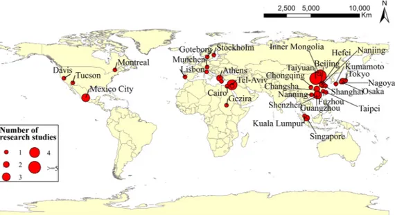
differences between the air temperature of vegetation and of open spaces used as reference. The reference land must be open spaces with non-vegetation. Field measurements were conducted on days with no rain and low wind speed. Based on the above criteria, a total of 3634 samples (Fig. S1) from 77 sites (44 sites with time-series and 33 in-dividual observations) in 35 cities worldwide were collected from the global published literature (Fig. 1, Supplementary dataset). Of the 77 sites, 29 are located in the tropics (0°N–23.5°N), 46 at northern tem-perate latitudes (23.5°N–50°N), and 2 are situated at northern boreal latitudes (50°N–60°N). None are located in the southern hemisphere. The data collected from the original literature contain mainly the fol-lowing fields: latitude, longitude, altitude, city, country, year, month, time, UTC time, observed ΔTa, BAT, vegetation type (seeSection 2.4)
and vegetation coverage area (S). The information of global in-situ sites are shown inTable 1.
To reduce potential error of ΔTacaused by the differences in
ob-servation height, which vary from 1.0 m to 2.0 m in the published lit-erature, we adopted the following methodologies to normalize the original ΔTaat different heights to those at 1.5 m:Lee et al. (2011)
evaluated the vertical Taabove tree canopy from a subset of forest sites
and found that Tawas not sensitive to observation height (<0.2 °C from
2–15 m above canopy), most likely due to a strong atmospheric mixing which is a universal characteristic of turbulent flow above forests. Here, we assumed that in-situ Tvegwithin forest systems also varies little from
1.0- to 2.0-m observations.Baum (1949)investigated the vertical gra-dients of mean daytime and nighttime in-situ Topenbetween 0.15 m and
1.5 m throughout a 12-month period (Tables 1and2,Baum, 1949). In this case, we simply assumed that Topenchanges homogeneously from
1.0 m to 2.0 m above open ground and calculated the average vertical
gradient (Table S1). The gradient was applied to convert the original values of Topento a normalized Topenat 1.5 m. Subsequently, T*a was correspondingly calculated by using Tvegminus normalized Topen.
Be-cause in-situ Tvegand Topenwere observed using the same sensor, we did
not consider the potential uncertainty that might have resulted from using different sensors. Furthermore, we took into account the most acknowledged BAT to represent background climate differences, ig-noring other microclimate variables such as wind, humidity and vapor pressure deficit, as we chose the records that collected under no-rain and low wind-speed weather.
2.2. Gridded datasets of vegetation and climate variables
Aside from the above in-situ observations, we supplemented vege-tation, phenology and climatic variables that were sampled from global gridded products by matching the locations of in-situ sites to gridded imageries, such as Enhanced Vegetation Index (EVI), Normalized Difference Vegetation Index (NDVI), Leaf Area Index (LAI), evapo-transpiration (ET), Plant Growth Stage (PGS, see Section 2.4), and downward solar shortwave radiation (∅). The data sources of gridded products of EVI, NDVI, LAI, ET, PGS and ∅ are listed inTable 2. We did not take into account the records before the year 2000 (13% of the total samples) for PGS and vegetation index - related analysis, as MODIS data are only available after 2000.
MODIS ET products (ETMODIS) were estimated using the improved ET algorithm byMu et al. (2011)instead of the earlierMonteith (1965) method. Also worthy of note is that the spatial resolution of the gridded MODIS EVI, NDVI, LAI, and ET products might be too low for in-situ site matching. To evaluate the potential uncertainty caused by the differ-ences between the footprint of MODIS products and the scale of in-situ observations, we used in-situ climate data to calculate monthly
ET (ETin situ) based on the Penman-Monteith equation (Houspanossian et al., 2013) for inter-comparison, which shows sa-tisfactory correlation performances against MODIS EVI, NDVI, LAI, and
ET products (R2= 0.33, 0.25, 0.19 and 0.32, respectively; p < 0.001)
(Fig. S2).
2.3. Proxies for three main functions – background climate, evaporative cooling, and canopy shading
Due to the complexity of climatic and vegetative factors in med-iating vegetation cooling and warming, for the three main functions – background climate, ET, and shading – we selected the most used proxies, as suggested by former studies.
- BAT as proxy of the background climate effect (Zhang et al., 2013; Zhao et al., 2014;Li et al., 2015);
- ETin stu as proxy of the vegetation evapotranspiration function (Taha et al., 1991; Bowler et al., 2010; Feyisa et al., 2014; Zhao et al., 2014);
- S as proxy of the canopy shading function (Oke, 1989; Pearlmutter et al., 1999;Dimoudi and Nikolopoulou, 2003).
Table 2
Data sources of gridded products of EVI, NDVI, LAI, ET, PGS, and ∅.
Name Products Version Spatial resolution Temporal resolution References
EVI MODIS Vegetation Indices (MOD13Q1) Collection 6 250 m 16-day Friedl et al. (2002)
NDVI MODIS Vegetation Indices (MOD13Q1) Collection 6 250 m 16-day Myneni et al. (2002)andFriedl et al. (2002)
LAI MCD15A3H MODIS/Terra+Aqua Leaf Area Index/FPAR
(MOD15A3H) Collection 6 500 m 4-day Myneni et al. (2002)
ET Global Terrestrial Evapotranspiration Data Set (MOD16A2) Collection 5 1 km 8-day Mu et al. (2011)
PGS MODIS Global Land Cover Dynamics Product (MCD12Q2) Collection 6 500 m 8-day Hufkens et al. (2012)
2.4. Attribution of three main cooling functions to temporal, spatial, vegetative and climatic drivers
Because the background climate, ET and shading functions are closely correlated, we decomposed them into independent underlying variables to gain insight on the drivers controlling T*a. The background climate is mainly determined by short-wave radiation, latitude, alti-tude, season, and time of day. The shading function is principally re-lated to vegetation area, type, vegetation indices (e.g., EVI), and tem-poral variations (Oke, 1989;Upmanis et al., 1998;Pearlmutter et al., 1999;Dimoudi and Nikolopoulou, 2003;Doick et al., 2014). Moreover, the vegetation evaporative function is related to PGS (Guimberteau et al., 2014), vegetation type (Zhang et al., 2001; Zhou et al., 2015), vegetation indices (e.g., EVI) (Buitenwerf et al., 2015;Wu et al., 2016), and solar radiation (Bi et al., 2015) as illustrated in Fig. S3.
To divide the daytime and nighttime periods, in this study we firstly used the local2Solar function in the solaR package to convert local time to UTC time. The R package solaR includes a set of classes, methods and functions to calculate sun geometry and the solar radiation incident (R Development Core Team, 2012). We further used the sunrise.set function in the StreamMetabolism package, which calculates sunrise and sunset times using MapTools based on the NOAA (National Oceanic and Atmospheric Administration) sunrise sunset calculator, to calculate sunrise and sunset times (Sefick, 2016). Based on this, we lastly dis-tinguished the daytime and nighttime periods for each day. In addition, the in-situ observations were classified into warm (i.e., May-Aug) and cool (i.e., Nov-Dec, Jan-Feb) seasons to illustrate the differences be-tween the two seasonal periods. To present the latitudinal patterns of vegetation cooling, we divided the samples into three broad latitude bands according to the following site locations: 30°S to 30°N (tropics), between 30° and 40° (temperate latitudes) and north of 40°N and south of 40°S (high latitudes). Vegetation was initially classified into three common types: forest, shrub, and grass. Of note, urban forests are mostly developed as defined block parks or striped greenways.
Therefore, in this study forests were further differentiated into tree block and tree row according to their shapes. The trees along boule-vards and rivers (e.g., greenways) are classified as tree rows, while those distributed as blocks (e.g., parks) are classified as tree blocks. The shrub reported in a single study (Li and Liang, 2007) was not con-sidered in the analysis. The PGS, which is a proxy of vegetation phe-nology, was divided into three stages: leaf growth, leaf senescence and dormancy, based on the seasonality of NDVI according to the method of Buitenwerf et al. (2015). The leaf growth stage indicates the period when new leaf onset is more abundant than old leaf drop, whereas the senescence stage is represented by greater old leaf shedding compared to new leaf flushing. The dormancy stage is the period with rare leaf onset and drop.
2.5. Statistical analyses
The bootstrap sampling has been widely used to randomly test the relationship between two dependent/independent variables, especially in meta-analysis studies (Dybala et al., 2019;Guerrero-Ramírez et al., 2019). We used the bootstrapping approach for slope analysis of T*a against the proxies of the three main functions – background climate, evaporative cooling, and canopy shading.
The hierarchical partitioning method (Walsh and Mac Nally, 2013) is a technique that involves collinearity to estimate the percentage of explained variance of each predictor variable into independent and joint contribution with all other variables, considering all possible models in a multivariate regression (Chevan and Sutherland, 1991; Pinkert et al., 2017). We used hierarchical partitioning in the hier.part R package to decompose for contribution analysis.
2.5.1. Bootstrapping methods for calculating slope analyses
For each of the above three variables (X), we initially used the bootstrapping method to randomly select a sample (Xi) of observations
with replacements from the original X dataset. We then sorted the X vector in ascending order based on the following rules: (1) the
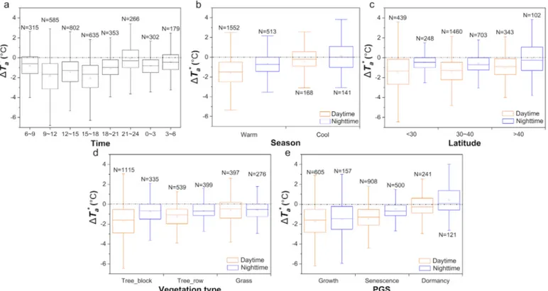
Fig. 2. Temporal, spatial and vegetative variability of mean T*a. (a) Diurnal cycle; (b) Seasonal variability; (c) Latitudinal pattern; (d) Vegetation types; (e) PGS
minimum number of Xiis >25% but <75% of the total number of X;
and (2) the range of Xiis >¼ of the full range of the sorted vector X. For
each bootstrap, we fitted a linear regression model between T*a and Xi
and calculated the slope of the corresponding linear regression model. For each Xi, 1000 bootstrap replicates were implemented in this
cal-culation.
2.5.2. Hierarchical partitioning for attributing contribution analysis
The hierarchical partitioning method first calculates the goodness-of-fit of models using all combinations of an independent variable. We then followed the method byWalsh and MacNally (2003)to estimate their contributions to the predictor variable. The hierarchical parti-tioning method implemented in the hier.part R package can compute the contributions of categorical variables and continuous variables to the dependent variable (see details inWalsh and MacNally, 2003). We conducted two processes of contribution analysis related to our two objectives:
- to calculate the contributions of the background climate forcing, evaporative cooling and canopy shading functions (i.e. proxies: BAT,
ETin stuand S variables, respectively) to T*a.
- to calculate the contributions of the nine factors mentioned above (latitude, altitude, season, time of day, ∅, vegetation type, S, EVI, and PGS) to T*a, herein termed as Clat, Calt, Csea, Ctim, C∅, Ctyp, CS, CEVI, and CPGS, respectively.
3. Results and discussion
3.1. Urban vegetation cooling and warming effects on local air temperature: temporal, spatial and vegetative variability
The T*a from global published literature varied greatly and ranged from −9.7 to 5.2 °C (Fig. S1). Overall, 80% of T*aobservations showed a cooling effect while only 16% demonstrated a warming effect, re-maining 4% showing no effect. Given that vegetation cooling and warming are dependent on or related to temporal and spatial factors, as well as vegetation states, we firstly present the general patterns of how
T*a varied with changes in time, seasons, latitudes, vegetation types and vegetation growth stages.
3.1.1. Temporal and spatial patterns
The diurnal cycle and seasonality were important temporal factors influencing the variability of vegetation cooling and warming (Fig. 2a and b). Urban vegetation tends to exert stronger cooling effects during the daytime period but reduced cooling and even warming effects during the nighttime period (Fig. S4). This difference between daytime and nighttime periods reached a significant level throughout the year (p ≤ 0.005, Table S2), except for winter. The strong cooling effects took place in the late morning, between 9:00 a.m. and 12:00 p.m. ( T*a= −1.8 ± 0.07 °C), and late afternoon, between 3:00 p.m. and 6:00 p.m. ( T*a= −2.0 ± 0.07 °C). It is worth noting that the cooling effect was slightly depressed in the early afternoon between 12:00 p.m. and 3:00 p.m. ( T*a= −1.4 ± 0.06 °C) (Fig. 2a). This phenomenon is possibly related to high temperature depression of photosynthesis ob-served in ecosystems (Taub et al., 2000; Yang et al., 2006), but not exactly consistent with the optimal theory of mid-day stomatal closure (Cowan and Farquhar, 1977). Because T*a was not only influenced by evaporative cooling but also by other factors. Besides, several former studies have indeed observed afternoon stomatal closure in different vegetation types (Sayre,1926; Tenhunen et al., 1982; Correia et al., 1990). Urban vegetation in the warm seasons contributed considerable cooling effects (daytime: T*a= −1.6 ± 0.04 °C; nighttime: T*a = −0.7 ± 0.08 °C) (Fig. 2b); however, no significant cooling ef-fect was observed in the cool seasons, especially during the nighttime period (daytime: T*a= −0.41 ± 0.13 °C; nighttime:
T*a = −0.09 ± 0.13 °C).
For spatial patterns, vegetation daytime cooling was related to la-titudes, producing a decreasing trend from the tropics ( T*a= −1.5 ± 0.09 °C) to the temperate ( T*a= −1.4 ± 0.04 °C), and to the high-latitude bands ( T*a= −1.0 ± 0.09 °C) (Fig. 2c). Greater differences between warm and cool seasons were observed in the higher latitudes (>40°N: T*a= −1.4 °C) and smaller differences in lower latitude zones (<30°N: T*a= −0.9 °C) (Fig. S5, Table S3).
Fig. 3. Associations of background air temperature (BAT) of urban areas (BAT), vegetation evapotranspiration calculated from in-situ data (ETin stu) and vegetation
area (S) with the normalized gradient ( T*)a between Tvegand Topen. (a–c) Box plots of T*a in various BAT, ETin situ, S ranges; (d–f) Linear regression slope of BAT,
3.1.2. Vegetative differences
Vegetation types and growth stages influence its cooling and warming effects. The vegetation daytime cooling level differed sig-nificantly among tree, shrub and grass lands (p < 0.001) (Fig. 2d, Table S4), with tree block ( T*a= −1.7 ± 0.05 °C) showing the maximum cooling, followed by tree row ( T*a= −1.3 ± 0.05 °C), while grass-land generated weaker cooling effect ( T*a= −0.6 ± 0.08 °C) com-pared with forest lands. There were no significant differences in nighttime T*a between tree block, tree row and grassland. Vegetation cooling/warming also co-varied with plant PGS (Fig. 2e), with max-imum cooling usually during the leaf growth period (daytime:
T*a= −1.7 ± 0.08 °C; nighttime: T*a= −1.5 ± 0.18 °C). This temperature mitigation decreased during the leaf senescence stage (daytime: T*a= −1.4 ± 0.04 °C; nighttime: T*a= −0.4 ± 0.06 °C), and reached the minimum during the dormancy stage (daytime: T*a= −0.1 ± 0.08 °C; nighttime: T*a= 0.4 ± 0.14 °C). At the growth (p = 0.362) and dormancy (p = 0.147) stages, there was no significant difference between day-time and nightday-time cooling (Table S5), whereas at the leaf senescence stage vegetation-induced cooling effect was significantly stronger during daytime than during nighttime (p < 0.001).
3.2. Associations of background climate, ET and shading functions with T*a
Regarding the diverse cooling and warming magnitudes, one of the most pressing issues to be addressed by the scientific community is the thresholds when vegetation performs cooling and warming effects in cites. Fig. 3 shows the box plots of T*a in various BAT, ETin stu, S ranges, and the slopes of corresponding simple linear regression models based on the bootstrapping method with 1000 replicates (see Section 2.4).
In general, the background climate plays an important role in de-termining whether vegetation cools or warms the air temperature. In cooler climate with daily BAT on average <10.0 °C (Fig. 3a), urban vegetation was associated with a small warming effect ( T*a = 0.4 ± 0.13 °C) (69% of the data). Sixty-seven percent of the samples with warming effects were observed during nighttime or during the cool seasons. When daily mean BAT was >10.0 °C, urban vegetation began to exert a cooling effect (average
T*a= −1.7 ± 0.06 °C) (Fig. 3a). Slope analysis of the fitting curve between T*a and daily mean BAT showed that the vegetation cooling effect becomes more sensitive to BAT increases when BAT was >25.7 °C (Fig. 3d). The meta-analysis above indicated that it is the BAT variable that mainly determines whether urban vegetation exerts a cooling or warming effect in urban areas, and that the cooling effect of urban vegetation is likely to increase in cities with high BAT. For ex-ample, the in-situ air temperature in Shenzhen's urban park in sub-tropical southern China (latitude: 113.97°N, longitude: 22.57°E) is 5.60 °C cooler than in open land during the hot summer season (BAT = 32.3 °C) (Lei et al., 2011). Conversely, the magnitude of
vegetation cooling is always less than 3.0 °C in northern Beijing city (latitude: 116.35°N; longitude: 40.00°E; BAT = 21.1 °C). This trend was also proven by the observations of former studies (Davenport and Hudson, 1967;Shashua-Bar et al., 2010;Chen et al., 2012;Cai et al., 2013), which concluded that background climate was the key influen-cing factor.
In contrast with the daily mean BAT, to each of the ETin stu range there always corresponded to a vegetation cooling effect (Fig. 3b). Only a moderate cooling effect was observed when ETin stuwas less. When ETin stu was >61.7 mm per month, the vegetation cooling effects started to become much stronger (Fig. 3e), especially when ETin stuwas >105.0 mm per month ( T*a = −2.4 ± 0.13°) (Fig. 3b). This finding indicated that the increase of ETin stu tended to produce a greater cooling effect under higher ETin stuconditions.
Similar to ETin stu, a moderate cooling effect ( T*a= −0.9 ± 0.08 °C) was observed when S was < 30.0 ha. When S became larger (S >30 ha), the vegetation cooling was greatly en-hanced, with an average T*a= −3.3 ± 0.32 °C (Fig. 3c). This more or less coincided with the slope analysis, which revealed a considerable break point of T*a against S before and after S = 35.2 ha (Fig. 3f).
To better illustrate the performance of vegetation functions in ex-erting the cooling and warming effects, we chose three most commonly selected proxies (i.e., BAT, ETin situand S variables) to represent the background climate, vegetation evaporative function and canopy
Fig. 4. Average contributions (C) of BAT, ETin situ, and shading effects to T*a.
Fig. 5. Contributions (C) of BAT, ETin situ, and shading effects to T*aalong with
various BAT ranges.
Fig. 6. Decomposition of the contributions of underlying factors to T*a. Clat,
Calt, Csea, Ctim, C∅, Ctyp, CS, CEVI, and CPGSare the relative contributions of
la-titude, alla-titude, season, time of day, ∅, vegetation type, S, EVI, and PGS to T*,a respectively.
shading function, respectively, and attributed their contributions (CBAT, CET, Cshading) to T*a with different background climates using the hierarchical partitioning method (seeSection 2.5). Our results showed that CBAT, CET and Cshading, on average, equaled 46.4 ± 0.10%,
40.4 ± 0.11% and 16.5 ± 0.13%, respectively (Fig. 4). Background climate was modeled as the most important function of vegetation cooling and warming, in comparison with evaporative cooling and ca-nopy shading.Fig. 5further shows how CBAT, CETand Cshadingvaried in
different BAT ranges. As BAT decreased, Cshadingdramatically increased,
while both CBATand CET decreased (Fig. 5). The shading function of
vegetation contributed the most in cites with a cooler climate (BAT <10.0 °C,Fig. 5).
These findings provide helpful information to gain a deeper un-derstanding of the relative importance of background climate and ve-getation functions in controlling cooling and warming effects.
3.3. Insights on the mechanisms of underlying factor impacts on background climate, evaporative cooling, and shading
To further investigate the underlying factors contributing to urban vegetation cooling and warming, we attributed the three functions (background climate, ET, and shading) to be comprehensively mediated by nine independent underlying factors (latitude, altitude, season, time of day, ∅, vegetation type, S, EVI, and PGS) (seeSection 2.4and Fig. S3). The contributions of these nine underlying factors to T*a were ranked by order of importance as: CPGS> Csea> Clat> CEVI> CS> Calt> C∅> Ctyp> Ctim(Fig. 6). The vegetation phenological proxy
-PGS (CPGS= 37.6 ± 0.11%) (i.e., growth, senescence and dormancy),
which contributed a large part to evaporative seasonality, acted as the primary biological factor influencing vegetation cooling and warming. Seasonality (Csea= 23.0 ± 0.11%) and latitude
(Clat= 11.4 ± 0.07%), which controlled background climate, were
two other important contributors. The EVI, to some extent representing the mean greenness of plant canopy, and vegetation area controlling shade cooling contributed 9.8 ± 0.08% and 6.3 ± 0.06%, respec-tively. The altitude (Calt= 3.7 ± 0.03%), mean ∅
(C∅= 3.5 ± 0.03%), vegetation type (Ctyp= 2.6 ± 0.04%) and time
period (Ctim= 2.1 ± 0.04%) played a much less important role.
Previous studies have mainly attributed vegetation cooling and warming to biological factors, such as vegetation indices (Zhang et al., 2013), vegetation types (Feyisa et al., 2014), and vegetation areas (Wong and Yu, 2005; Chang et al., 2007; Cao et al., 2010a,b; Chen et al., 2012). However, by further decomposing the contributions of independent underlying factors to vegetation cooling and warming effects, the vegetation phenological proxy - plant growth stage is modeled in our study as the most important biological contributor. This is probably because vegetation phenology (i.e., leaf onset and litterfall) controls the seasonality of canopy activity, for example, leaf photo-synthesis (Wu et al., 2016), plant transpiration (Li et al., 2015; Zipper et al., 2017), as well as canopy cover (Peng et al., 2014) and leaf areas (Zeng et al., 2017) – all of which would considerably impact on vegetation cooling and warming. Especially, under the effects of the urban heat island (UHI), vegetation tends to release more water through transpiration during the leaf growth stage and in turn exerts stronger cooling effects on the local climate (Zipper et al., 2017). The leaf growth stage is expected to be enhanced and extended as a result of extremely extreme high air temperatures (Parece and Campbell, 2018; Walker et al., 2015;Li et al., 2017; Zipper et al., 2016; Jochner and Menzel, 2015). From a more critical standpoint, with the increase of UHI effects, the plant phenology will become increasingly effective in controlling the vegetation cooling and warming. This might in turn undermine the seasonality and latitudinal patterns of vegetation cooling and warming (Lee et al., al.,2011;Zeng et al., al.,2017).
4. Conclusions
This analysis of the first global dataset of vegetation cooling and warming effects on urban air temperature indicate that although ve-getation generally results in a cooling effect, its direction and magni-tude show considerable temporal, spatial and vegetative variations. The background climate, evaporative cooling and canopy shading are three important functions that drive the vegetation cooling and warming. Importantly, this study notes several thresholds: vegetation cooling begin when background air temperature exceeds 10 °C; evaporative cooling increases when evapotranspiration exceeds 62.7 mm per month; and shading cooling increases sharply when vegetated area exceeds 35.2 ha. The vegetation phenology proxy (i.e., growth stages: leaf growth, leaf senescence and dormancy) (CPGS= 37.6 ± 0.11%)
acts as the primary biotic factor, while seasonality (Csea= 23.0 ± 0.11%) and latitudes (Clat= 11.4 ± 0.07%) are two
highly important abiotic contributors.
Overall, our findings are important for assessing the effects of ve-getation cooling and warming on urban air temperature and providing useful information for future urban greenspace planning aimed at mi-tigating local warming conditions. To produce maximum vegetation cooling on local climate, it is suggested to plant vegetations with the leaf growth stage coinciding with the warm season periods. This is particularly important for tropical and subtropical regions, where are mainly covered by the evergreen-canopy vegetations with complex canopy phenology. Note also that there might still be some uncertainty caused by observation methodologies, sensors and climatic variability such as wind, humidity, and vapor pressure deficit. More intensive observations are warranted from global in-situ sites using consistent methods.
Acknowledgements
We thank the editor and reviewers for their valuable comments to improve the manuscript. This study was supported by the National Natural Science Foundation of China [grant nos. 41971275, 31971458, 41430529], Special high-level plan project of Guangdong Province [grant no. 2016TQ03Z354], the Pearl River S&T Nova Program of Guangzhou [grant no. 201610010134], and the GDAS’ project of Science and Technology Development [grant numbers 2016GDASRC-0101, 2017GDASCX-0101, 2017GDASCX-0501, 2019GDASYL-0103002].
Supplementary materials
Supplementary material associated with this article can be found, in the online version, atdoi:10.1016/j.agrformet.2019.107765.
References
Ahmad, S.A., 1992. Some effects of urban parks on air temperature 6ariations in Kuala Lumpar, Malaysia. In: Paper presented at the 2nd Tohwa University International Symposium, CUTEST’92, 7–10 September 1992. Fukuoka, Japan. 1992. Tohwa Institute for Sciences, Tohwa University, pp. 107–108 Preprints from.
Alkama, R., Cescatti, A., 2016. Biophysical climate impacts of recent changes in global forest cover. Science 351 (6273), 600–604.
Bacci, L., Morabito, M., Raschi, A., Ugolini, F. (2003). Thermohygrometric Conditions of Some Urban Parks of Florence (Italy) and their Effects on Human Well-being. In: Paper pre.
Barradas, V.L., 1991. Air temperature and humidity and human comfort index of some city parks of Mexico City. Int. J. Biometeorol. 35 (1), 24–28.
Baum, W.A., 1949. On the relation between mean temperature and height in the layer of air near the ground. Ecology 30 (1), 104–107.
Bi, J., Knyazikhin, Y., Choi, S., Park, T., Barichivich, J., Ciais, P., ... Huete, A., 2015. Sunlight mediated seasonality in canopy structure and photosynthetic activity of Amazonian rainforests. Environ. Res. Lett. 10 (6), 064014.
Bonan, G.B., 2008. Forests and climate change: forcings, feedbacks, and the climate benefits of forests. Science 320 (5882), 1444–1449.
Bounoua, L., Defries, R., Collatz, G.J., Sellers, P., Khan, H., 2002. Effects of land cover conversion on surface climate. Clim. Change 52 (1–2), 29–64.
Bowler, D.E., Buyung-Ali, L., Knight, T.M., Pullin, A.S., 2010. Urban greening tocool towns and cities: a systematic review of the empirical evidence. Landsc. Urban Plan. 97, 147–155.
Bru¨ndl, W., Mayer, H., Baumgartner, A., 1986. Untersuchung Des Einflusses 6on Bebanung Und Bewachs Auf Das Klima Und Die Lufthygienischen 6erhaltnisse in Bayerischen grosstadted, Stadtklima Bayern, Abschlussbericht zum Teilprogramm ‘Klimamessungen Munchen’. Lehrstuhl fur Bioklimatologie und Angewandte Meteorologie der Universitat Munchen (in German).
Buitenwerf, R., Rose, L., Higgins, S.I., 2015. Three decades of multi-dimensional change in global leaf phenology. Nat. Clim. Change 5 (4), 364.
Ca, V.T., Asadea, T., Abu, E.M., 1998. Reductions in air conditioning energy caused by a nearby park. Energy Build. 29, 83–92.
Cai, Y., Yan, S., Chen, Y., Lei, S., Ye, W., 2013. Effects of different structures of green belts on the temperature and humidity in river corridors of subtropical cities. J. Fujian Coll. Forestry 33 (4), 357–362 (in chinese).
Cao, X., Onishi, A., Chen, J., Imura, H., 2010a. Quantifying the cool island intensity of urban parks using ASTER and IKONOS data. Landsc. Urban Plan. 96 (4), 224–231.
Cao, X., Onishi, A., Imurab, H., 2010b. Quantifying the cool island intensity of urban parks using ASTER and IKONOS data. Landsc. Urban Plan. 96, 224–231.
Chang, C.R., Li, M.H., Chang, S.D., 2007. A preliminary study on the local cool-island intensity of Taipei city parks. Landsc. Urban Plan. 80, 386–395.
Chen, X.Z., Su, Y.X., Li, D., Huang, G.Q., Chen, W.Q., Chen, S.S., 2012. Study on the cooling effects of urban parks on surrounding environments using Landsat TM data: a case study in Guangzhou, southern China. Int. J. Remote Sens. 33 (18), 5889–5914.
Chevan, A., Sutherland, M., 1991. Hierarchical partitioning. Am. Stat. 45, 90–96.
Cohen, J.L., Furtado, J.C., Barlow, M.A., Alexeev, V.A., Cherry, J.E., 2012. Arctic warming, increasing snow cover and widespread boreal winter cooling. Environ. Res. Lett. 7 (1), 014007.
Correia, M.J., Chaves, M.M.C., Pereira, J.S., 1990. Afternoon depression in photosynthesis in grapevine leaves—evidence for a high light stress effect. J. Exp. Bot. 41 (4), 417–426.
Cowan, I.R., Farquhar, G.D., 1977. Stomatal function in relation to leaf metabolism and environment. Symp. Soc. Exp. Biol. 31, 471.
d'Amour, C.B., Reitsma, F., Baiocchi, G., Barthel, S., Güneralp, B., Erb, K.H., Haberl, H., Creutzig, F., Seto, K.C., 2016. Future urban land expansion and implications for global croplands. In: Proceedings of the National Academy of Sciences, , 201606036.
https://doi.org/10.1073/pnas.1606036114.
Davenport, D.C., Hudson, J.P., 1967. Local advection over crops and fallow 1 changes in evaporation rates along a 17-km transect in the Sudan Gezira. Agric. Meteorol. 4 (5), 339–352.
Dhakal, S., Hanaki, K., 2002. Improvement of urban thermal environment by managing heat discharge sources and surface modification in Tokyo. Energy Build. 34 (1), 13–23.
Dimoudi, A., Nikolopoulou, M., 2003. Vegetation in the urban environment: microcli-matic analysis and benefits. Energy Build. 35, 69–76.
Doick, K.J., Peace, A., Hutchings, T.R., 2014. The role of one large greenspace in miti-gating London's nocturnal urban heat island. Sci. Total Environ. 493, 662–671.
Dybala, K.E., Matzek, V., Gardali, T., Seavy, N.E., 2019. Carbon sequestration in riparian forests: a global synthesis and meta‐analysis. Glob. Change Biol. 25 (1), 57–67.
Ellison, D., Morris, C.E., Locatelli, B., Sheil, D., Cohen, J., Murdiyarso, D., Gaveau, D., 2017. Trees, forests and water: cool insights for a hot world. Glob. Environ. Chang. 43, 51–61.
Escobedo, F.J., Kroeger, T., Wagner, J.E., 2011. Urban forests and pollution mitigation: analyzing ecosystem services and disservices. Environ. Pollut. 159 (8), 2078–2087.
Feng, Y.L., 2008. Study on effect of reducing temperature and increasing humidity in gardening plant community in Chongqing city. J. Anhui Agric. Sci.
Feyisa, G.L., Dons, K., Meilby, H., 2014. Efficiency of parks in mitigating urban heat island effect: an example from Addis Ababa. Landsc. Urban Plan. 123, 87–95.
Friedl, M.A., McIver, D.K., Hodges, J.C.F., Zhang, X.Y., Muchoney, D., Strahler, A.H., et al., 2002. Global land cover mapping from MODIS: Algorithms and early results. Remote Sens. Environ. 83 (1–2), 287–302.
Georgi, J.N., Dimitriou, D., 2010. The contribution of urban green spaces to the im-provement of environment in cities: case study of chania, greece. Build. Environ. 45 (6), 1401–1414.
Georgi, N.J., Zafiriadis, K., 2006. The impact of park trees on microclimate in urban areas. Urban Ecosyst. 9, 195–209.
Guerrero-Ramírez, N.R., Reich, P.B., Wagg, C., Ciobanu, M., Eisenhauer, N., 2019. Diversity‐dependent plant–soil feedbacks underlie long‐term plant diversity effects on primary productivity. Ecosphere 10 (4), e02704.
Guimberteau, M., Ducharne, A., Ciais, P., Boisier, J.P., Peng, S., De Weirdt, M., Verbeeck, H., 2014. Testing conceptual and physically based soil hydrology schemes against observations for the Amazon Basin. Geosci. Model Dev. 7, 1115–1136.
Hamada, S., Ohta, T., 2010b. Seasonal variations in the cooling effect of urban green areas on surrounding urban areas. Urban Forestry Urban Green. 9, 15–24.
Houspanossian, J., Nosetto, M., Jobba′gy, E.G., 2013. Radiation budget changes with dry forest clearing in temperate Argentina. Glob. Change Biol. 19, 1211–1222.
Huang, L.M., Huang, Y.Y., Li, H., Li, J.L., 2007. Spatiotemporal dynamic analysis of mi-croclimatic factors in different types of urban greening areas during hot weather. Urban Environ.Urban Ecol. 20 (1), 29–34.
Huang, L.M., Li, J.L., Zhao, D.H., Zhu, J.Y., 2008. A fieldwork study on the diurnal changes of urban microclimate in four types of ground cover and urban heat island of Nanjing, China. Build. Environ. 43, 7–17.
Hufkens, K., Friedl, M.A., Keenan, T.F., Sonnentag, O., Bailey, A., O'keefe, J., Richardson, A.D., 2012. Ecological impacts of a widespread frost event following early spring leaf‐out. Glob. Change Biol. 18 (7), 2365–2377.
Jansson, C., Jansson, P.E., Gustafsson, D., 2007. Near surface climate in an urban
vegetated park and its surroundings. Theor. Appl. Climatol. 89 (3–4), 185–193.
Jauregui, E., 1991. Influence of a large urban park on temperature and convective pre-cipitation in a tropical city. Energy Build. 15 (3), 457–463.
Ji, P., Zhu, C.Y., H, S., 2012. Effects of urban river width on the temperature and humidity of nearby green belts in summer. Chin. J. Appl. Ecol. 23 (3), 679–684.
Jochner, S., Menzel, A., 2015. Urban phenological studies - past, present, future. Environ. Pollut. 203, 250–261.https://doi.org/10.1016/j.envpol.2015.01.003.
Jonsson, P., 2004. Vegetation as an urban climate control in the subtropical city of Gaborone, Botswana. Int. J. Climatol. 24, 1307–1322.
Lee, X., Goulden, M.L., Hollinger, D.Y., Barr, A., Black, T.A., Bohrer, G., ... Katul, G., 2011. Observed increase in local cooling effect of deforestation at higher latitudes. Nature 479 (7373), 384–387.
Lei, J.L., Tao, L., Wu, Y.Y., Zhang, X.Y., Xie, L.S., 2011. Effects of structure characteristics of urban green land on the temperature-lowering in Shenzhen city. J. Northwest Forestry Univ. 26 (4), 218–223.
Li, Y.D., Han, X.M., Wu, X.G., Hao, X.Y., Wang, J., Liang, F., Liang, J., Wang, Z.H., 2006a. Ecological field characteristic of green land based on urban green space structure. Acta Ecologica Sinica 26 (10), 3339–3346.
Li, Y.D., Wu, X.G., Hao, X.Y., 2006b. The response of boundary ecological effect to the structure of urban green space. Chin. Landsc. Archit. 22 (9), 73–76.
Li, H., Zhao, W.Z., Gu, R.Z., Li, Y.M., Chen, Z.X., Zhang, X.X., 1999. Effects of three different green-lands in plantation structure on the O2-emitting, CO2-fixing,
heat-absorbing and temperature-decreasing in residential quarters. Environ. Sci. 20, 41–44.
Li, X., Zhou, Y., Asrar, G.R., Mao, J., Li, X., Li, W., 2017. Response of vegetation phe-nology to urbanization in the conterminous United States. Glob. Change Biol. 23 (7), 2818–2830.https://doi.org/10.1111/gcb.13562.
Li, Y., Liang, F., 2007. Spatial and temporal distribution of microclimate effects of the urban shrub community. Chin. Agric. Sci. Bull. 23 (3), 313–317 (in chinese).
Li, Y., Zhao, M., Motesharrei, S., Mu, Q., Kalnay, E., Li, S., 2015a. Local cooling and warming effects of forests based on satellite observations. Nat. Commun. 6, 6603.
Liang, J., Li, Y.D., 2007. Temporal and spatial patterns of peripheral environment in-fluenced by urban forest. Chin. Agric. Sci. Bull. 23 (7), 379–385.
Liu, J., Li, S., Yang, Z., 2008. Temperature and humidity effect of urban green spaces in Beijing in summer. Chin. J. Ecol. 27 (11), 1972–1978.
Liu, X., 2004. Studies on Area Climate Effect of Greenbelt System and Landscape Ecology Construction of Urban of Hefei. Anhui Agricultural University, Hefei.
Luo, X., 2013. Efficiency of Temperature and Humidity in Changsha Urban Forests. Central South University of Forestry and Technology.
Ma, X.M., Li, J.Y., 2007. Influences of different green lands on urban microclimate. Hebei J. Forestry Orchard Res. 22 (2), 210–226.
Ma, X.Z., Li, C.S., Da, W.Y., 2010. The effects of reducing temperature and increasing humidity by different green lands in inner mongolia agricultural university. J. Inner Mong. Agric. Univ (Natural Science Edition).
Mahmoud, A.H.A., 2011. Analysis of the microclimatic and human comfort conditions in an urban park in hot and arid regions. Build. Environ. 46 (12), 2641–2656.
Meier, A.K., 1991. Measured cooling savings from vegetative landscaping. In: Vine, E., Crawley, D., Centolella, P. (Eds.), Energy Efficiency and the Environment: Forging the Link. American Council for an Energy Efficient Economy, Washington, DC, pp. 321–334.
Monteith, J.L., 1965. Evaporation and environment. In: Fogg, B.D. (Ed.), The State and Movement of Water in Living Organism, Symposium of the Society of Experimental Biology 19. Cambridge University Press, Cambridge, pp. 205–234 (1965).
Mu, Q., Zhao, M., Running, S.W., 2011. Improvements to a MODIS global terrestrial evapotranspiration algorithm. Remote Sens. Environ. 115 (8), 1781–1800.
Myneni, R.B., Hoffman, S., Knyazikhin, Y., Privette, J.L., Glassy, J., Tian, Y., et al., 2002. Global products of vegetation leaf area and fraction absorbed PAR from year one of MODIS data. Remote Sens. Environ. 83 (1–2), 214–231.
Nakayama, T., Fujita, T., 2010. Cooling effect of water-holding pavements made of new materials on water and heat budgets in urban areas. Landsc. Urban Plan. 96 (2), 57–67.
Oke, T.R., 1989. The micrometeorology of the urban forest. Philos. Trans. R. Soc. B 324, 335–349.
Oliveira, S., Andrade, H., Vaz, T., 2011. The cooling effect of green spaces as acon-tribution to the mitigation of urban heat: a case study in Lisbon. Build. Environ. 46, 2186–2194.
Parece, T.E., Campbell, J.B., 2018. Intra-Urban microclimate effects on phenology. Urban Sci. 2 (1), 26.https://doi.org/10.3390/urbansci2010026.
Pearlmutter, D., Bitan, A., Berliner, P., 1999. Microclimatic analysis of “compact”urban canyons in an arid zone. Atmos. Environ. 33, 4143–4150.
Peng, S.S., Piao, S., Zeng, Z., Ciais, P., Zhou, L., Li, L.Z., Myneni, R.B., Yin, Y., Zeng, H., 2014. Afforestation in China cools local land surface temperature. In: Proceedings of the National Academy of Sciences. 111. pp. 2915–2919.
Pinkert, S., Brandl, R., Zeuss, D., 2017. Colour lightness of dragonfly assemblages across North America and Europe. Ecography 40 (9), 1110–1117.
Potchter, O., Cohen, P., Bitan, A., 2006a. Climatic behavior of various urban parks during a hot and humid summer in the Mediterranean city of Tel Aviv, Israel. Int. J. Climatol. 26, 1695–1711.
Potchter, O., Goldman, D., Iluz, D., Kadish, D., 2012. The climatic effect of a manmade oasis during winter season in a hyper arid zone: the case of southern israel. J. Arid Environ. 87 (12), 231–242.
R Development Core Team, 2012. R: a language and environment for statistical com-puting. R Foundation for Statistical Computing, Vienna, Austria. ISBN 3-900051-07-0, URL. http://www.R-project.org/.
Ruane, A.C., Goldberg, R., Chryssanthacopoulos, J., 2015. Climate forcing datasets for agricultural modeling: Merged products for gap-filling and historical climate series
estimation. Agric. Meteorol. 200, 233–248.
Sayre, J.D. (1926). Physiology of STOMATA OF RUMEX Patientia.
Sefick, S. Jr. (2016). Stream Metabolism-a Package for Calculating Single Station Metabolism from Diurnal oxygen Curves R Package version 1.1.2.
Seto, K.C., Güneralp, B., Hutyra, L.R., 2012. Global forecasts of urban expansion to 2030 and direct impacts on biodiversity and carbon pools. In: Proceedings of the National Academy of Sciences. 109. pp. 16083–16088.
Shashuabar, L., Hoffman, M.E., 2002. The green cttc model for predicting the air tem-perature in small urban wooded sites. Build. Environ. 37 (12), 1279–1288.
Shashua-Bar, L., Pearlmutter, D., Erell, E., 2009. The cooling efficiency of urban land-scape strategies in a hot dry climate. Landsc. Urban Plan. 92, 179–186.
Shashua-Bar, L., Tsiros, I.X., Hoffman, M.E., 2010. A modeling study for evaluating passive cooling scenarios in urban streets with trees. Case study: Athens, Greece. Build. Environ. 45, 2798–2807.
Spronken-Smith, R.A., Oke, T.R., 1998. The thermal regime of urban parks in two cities with different summer climates. Int. J. Remote Sens. 19, 2085–2104.
Su, Y., Liu, L., Wu, J., Chen, X*., Shang, J., Ciais, P., Zhou., G., Lafortezza, R., Wang, Y., Yuan, W., Zhang, H., Huang, G., Huang, N., 2019. Quantifying the biophysical effects of forests on local air temperature using a novel three-layered energy balance model. Environ. Int. 132, 105080.
Su, Y.X., Huang, G.Q., Chen, X.Z., Chen, S.S., 2010. Study on the cooling effect of Guangzhou city parks to surrounding environments. Acta Ecologica Sinica 30 (18), 4905–4918.
Sun, Y., Zhang, X., Ren, G., Zwiers, F.W., Hu, T., 2016. Contribution of urbanization to warming in China. Nat. Clim. Change 6, 706–709.https://doi.org/10.1038/ nclimate2956.
Susca, T., Gaffin, S.R., Dell'Osso, G.R., 2011. Positive effects of vegetation: urban heat island and green roofs. Environ. Pollut. 159, 2119–2126.
Taha, H., Akbari, H., Rosenfeld, A., 1991. Heat island and oasis effects of vegetative canopies: micro-meteorological field-measurements. Theor. Appl. Climatol. 44 (2), 123–138.
Tang, L.Z., Li, Z.Q., Yan, C.F., Sun, C.H., Xu, X., Xiang, H.R., 2009. Mitigative effects of different vegetations on heat island effect in Nanjing. Ecol. Environ. Sci. 18 (1), 23–28.
Taub, D.R., Seemann, J.R., Coleman J., S, 2000. Growth in elevated CO2protects
pho-tosynthesis against high‐temperature damage. Plant Cell Environ. 23 (6), 649–656.
Tenhunen, J.D., Lange, O.L., Jahner, D., 1982. The control by atmospheric factors and water stress of midday stomatal closure in Arbutus unedo growing in a natural macchia. Oecologia 55 (2), 165–169.
Upmanis, H., Eliasson, I., Lindqvist, S., 1998a. The influence of green areas on nocturnal temperatures in a high latitude city (Göteborg, Sweden). Int. J. Climatol. 18 (6), 681–700.
Walker, J.J., de Beurs, K.M., Henebry, G.M., 2015. Land surface phenology along urban to rural gradients in the U.S. Great Plains. Remote Sensing of Environment 165, 42–52.
https://doi.org/10.1016/j.rse.2015.04.019.
Walsh, C. & Mac Nally, R. (2013). Hier.Part: hierarchical Partitioning. R Package version 1.0-4.https://CRAN.R-project.org/package=hier.part.
Walsh, C., Mac Nally, R., 2003. The Hier. Part Package: Hierarchical Partitioning. Part of: Documentation for R: A Language and Environment for Statistical Computing.). R Foundation for Statistical Computing, Vienna, Austria URL. http://cran.r-project. org/web/packages/hier.part/hier.part.pdf.
Wang, J., Li, Y.D., 2004. The ecology effects of urban green spaces. Grassland Turf. 4, 24–27.
Wang, Y.X., Dong, J.W., Wang, Y.Z., Wang, N.S., 2005. Relationship between city green land and urban heat island effect. Subtrop. Plant Sci. 34 (4), 55–59.
Wolff, N.H., Masuda, Y.J., Meijaard, E., Wells, J.A., Game, E.T., 2018. Impacts of tropical deforestation on local temperature and human well-being perceptions. Glob. Environ. Chang. 52, 181–189.
Wong, N.H., Yu, C., 2005. Study of green areas and urban heat island in a tropical city. Habitat Int. 29 (3), 547–558.
Wu, P.F., Wang, M.J., Zhang, X.X., 2009. Relationship between vegetation greenness and urban heat island effect in Beijing. J. Beijing Forestry Univ. 31 (5), 54–60.
Wu, X.G., Lin, Y.D., Yan, H.B., Hao, X.Y., 2008. Correlation between ecological effect and structure characteristics of urban green areas. Chin. J. Eco-Agric. 16 (6), 1469–1473.
Wu, J., Albert, L.P., Lopes, A.P., Restrepo-Coupe, N., Hayek, M., Wiedemann, K.T., ... Tavares, J.V., 2016. Leaf development and demography explain photosynthetic sea-sonality in Amazon evergreen forests. Science 351 (6276), 972–976.
Yan, H., Wang, X., Hao, P., Dong, L., 2012. Study on the microclimatic characteristics and human comfort of park plant communities in summer. Procedia Environ. Sci. 13 (none), 755–765.
Yang, X., Chen, X., Ge, Q., Li, B., Tong, Y., Zhang, A., Li, Z., Kuang, T., Lu, C., 2006. Tolerance of photosynthesis to photoinhibition, high temperature and drought stress in flag leaves of wheat: a comparison between a hybridization line and its parents grown under field conditions. Plant Sci. 171 (3), 389–397.
Yu, C., Wong, N.H., 2006. Thermal benefits of city parks. Energy Build. 38, 105–120.
Zeng, Z., Piao, S., Li, L.Z., Zhou, L., Ciais, P., Wang, T., ..., Mao, J., 2017. Climate miti-gation from vegetation biophysical feedbacks during the past three decades. Nat. Clim. Change 7 (6), 432.
Zhang, L., Dawes, W.R., Walker, G.R., 2001. Response of mean annual evapotranspiration to vegetation changes at catchment scale. Water Resour. Res. 37, 701–708.
Zhang, M., Lee, X., Yu, G., Han, S., Wang, H., Yan, J., Kim, J., 2014. Response of surface air temperature to small-scale land clearing across latitudes. Environ. Res. Lett. 9 (3), 034002.
Zhang, M.L., Qin, Jun, 2008. Effects of temperature reduction and humidity increase of plant communities in shanghai. J. Beijing Forestry Univ. 30 (2), 39–43.
Zhang, Z., Lv, Y., Pan, H., 2013a. Cooling and humidifying effect of plant communities in subtropical urban parks. Urban forestry & urban greening 12 (3), 323–329.
Zhao, L., Lee, X., Smith, R.B., Oleson, K., 2014. Strong contributions of local background climate to urban heat islands. Nature 511 (7508), 216–219.
Zhao, S., Liu, K.W., Bi, Y.X., 2007. Reduction of different green lands on heat island effect in Changsha city. Acta Agric. Jiangxi 19 (9), 50∼52.
Zhou, G.Y., Wei, X.H., Chen, X.Z., Zhou, P., Liu, X.D., Xiao, Y., Sun, G., Scott, D., Zhou, S.Y.D., Han, L.S., Su, Y.X., 2015. Global pattern for the effect of climate and land cover on water yield. Nat. Commun. 6, 5918.http://dx.doi.org/10.1038/ ncomms6918.
Zhu, C.Y., L. I., H.S., Ji, P., 2011. Relationships between urban green belt structure and temperature-humidity effect. Chin. J. Appl. Ecol. 22 (5), 1255–1260.
Zipper, S.C., Schatz, J., Kucharik, C.J., Loheide, S.P., 2017. Urban heat island-induced increases in evapotranspirative demand. Geophys. Res. Lett. 44 (2), 2016GL072190.
https://doi.org/10.1002/2016GL072190.
Zipper, S.C., Schatz, J., Singh, A., Kucharik, C.J., Townsend, P.A., Loheide, S.P., 2016. Urban heat island impacts on plant phenology: intra-urban variability and response to land cover. Environ. Res. Lett. 11 (5), 054023. https://doi.org/10.1088/1748-9326/11/5/054023.
Zoulia, I., Santamouris, M., Dimoudi, A., 2009. Monitoring the effect of urban green areas on the heat island in Athens. Environ. Monit. Assess. 156 (1–4), 275.