If you can’t explain it simply,
you don’t understand it well enough.
Albert Einstein
A mia nonna Angela.
Per il suo volermi bene incondizionato e la felicit`
a
che mi trasmette ogni volta che mi `
e accanto.
Preface
Social networks became in recent years the most popular platforms for inter-action, communication and collaboration between friends. Indeed, they allow people to improve their social connection and to know political and social change almost instantaneously. Moreover, individual entertainment in a wide variety of forms is supported. Social networks also have a great impact in daily life due, in particular, to their effect on the way people are connected each other and can share valuable experiences, disseminate good practices, organize demonstrations and so on. In this respect, significant work on social networks has been done by sociologists and social psychologists since the 1950s, though almost all of this research was carried out on small-scale networks, because of the inherent difficulty of getting reliable, large-scale data from subjects about their friendships.
Nowadays, internet provides a new opportunity to study social interactions on a much larger scale than was previously possible. More in detail, we now have access to large-scale data on interactions and acquaintanceships. Indeed the size of social networks that can be studied has exploded from the hundreds of people to the hundreds of thousands of people or even more. As a result, there are new challenges tied to social networks management such as the efficient computation and maintenance of shortest distances in the network.
In this thesis, we study several questions about social networks from an algorithmic perspective.
In particular, we present two main contributions to the study of social networks:
1. The definition of an effective and efficient technique for shortest distances maintenance;
2. The study of a new and challenging problem such as the non progressive influence maximization.
Our contributions consist both in theoretical discussion on the topics, anal-ysis of related work and finally definition of suitable algorithms. Indeed, we will provide the reader a complete tool for understanding the basic notion
Preface VII of social networks, shortest paths and social influence, that will guide her through the comprehension of their underlying properties and algorithms. Organization
This thesis is organized into three parts. Part I is a background on social networks. We begin with discussing some structural properties to move then on to the question of social influence and its effectiveness. In part II we describe the challenging related to the shortest distance evaluation problem on the actual graphs, highlighting limits of the current solutions. We discuss our proposal to efficiently maintain all-pairs shortest distances for graphs stored in relational databases. Finally, part III continues the analysis introduced in part I but at the more fine-grained level of viral marketing. We introduce the influence maximization problem and some of its extensions considered in literature, before concluding with the discussion of a brand new relevant problem and our solution to solve it.
Summary of Publications
The results presented in part II of this thesis will appear in the Journal of Computer and System Sciences (JCSS 2015). Results reported in part III have been submitted to a top conference and are currently undergoing the review process.
Ringraziamenti
La tesi `e la sintesi di un percorso di studi, ma anche di vita. E scrivere questa sezione mi mette sempre in grossa difficolt`a..perch´e non `e facile riuscire a ringraziare in poche parole e senza scadere nelle classiche frasi fatte e di circostanza tutti coloro che mi hanno aiutato e supportato in questi anni. Ringrazio la mia famiglia, che, nonostante gli alti e gli innumerevoli bassi, mi `e sempre stata a suo modo vicina. Soprattutto durante i mesi all’estero, con le telefonate giornaliere di ore che facevano tanto sorridere i miei amici canadesi..a pensarci adesso mi stupisco di come ci fosse sempre, da un giorno all’altro, qualcosa di nuovo da raccontare!
Grazie ai miei “soci” Elio e Nunzio per la vostra amicizia e l’enorme pazienza dimostrata, soprattutto negli ultimi tempi.
Ringrazio i miei colleghi Deborah, Roberto e Salvatore perch´e avete reso questi anni di dottorato pi`u leggeri e pieni di risate. Un ringraziamento particolare a Cristian Molinaro per tutto l’aiuto, i consigli e soprattutto l’incoraggiamento durante le varie prove sostenute.
Il ringraziamento pi`u sincero va al mio supervisore Prof. Sergio Greco. In questi 10 anni qui all’universit`a, sei sempre stato per me un punto di riferi-mento e un modello da seguire. Perch´e nonostante il ruolo che rivesti, mi ha
VIII Preface
sempre colpito l’umilt`a con cui affronti le cose e il modo in cui riesci a mettermi a mio agio anche nei momenti in cui mi sembrava di non aver fatto abbastanza. Non finir`o mai di ringraziarti per la fiducia accordatami e l’opportunit`a che mi hai dato nel fare questo dottorato proprio con te.
Contents
Part I Social Networks
1 General Keynotes . . . 2
1.1 Structural Properties . . . 2
1.1.1 Scale Free Networks . . . 2
1.1.2 Small World Phenomenon . . . 3
1.2 Information and Influence Diffusion . . . 5
1.2.1 Social Influence . . . 6
Part II Shortest Distances Management in Large Networks 2 Shortest Distances Problem . . . 10
2.1 Definition . . . 11
2.2 Non Incremental Algorithms . . . 11
2.2.1 Limits . . . 11
2.3 Incremental Algorithms . . . 12
3 Shortest Distances Maintenance on DBMS . . . 15
3.1 Preliminaries . . . 15
3.2 Incremental Maintenance of All-Pairs Shortest Distances . . . 17
3.2.1 Single Edge Management . . . 19
3.2.2 Multiple Edges Management . . . 27
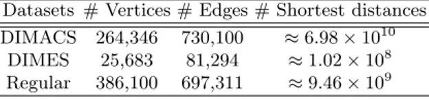
3.3 Experimental Evaluation . . . 33
3.3.1 Datasets . . . 33
3.3.2 Experimental setup . . . 35
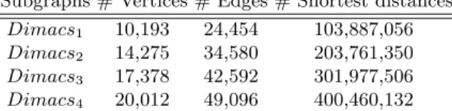
3.3.3 Results on the DIMACS dataset . . . 36
3.3.4 Results on the DIMES dataset . . . 39
3.3.5 Results on the regular dataset . . . 41
X Contents
Part III Non-Progressive Models for Viral Marketing in Social Networks
4 Influence Maximization Problem . . . 45
4.1 Modeling Cascading Behavior . . . 45
4.1.1 Independent Cascade Model . . . 46
4.1.2 Linear Threshold Model . . . 48
4.2 Problem Statement . . . 50
4.2.1 Greedy Algorithm for Influence Maximization . . . 51
4.3 Extensions . . . 52
4.3.1 Influence Maximization under Competition . . . 53
4.3.2 Continuous-Time Diffusion Process. . . 54
5 Competitive, Continuous Time and Non-Progressive Influence Maximization . . . 56
5.1 Problem Statement and Related Works . . . 57
5.1.1 Non-Progressive Influence Maximization Problem . . . 58
5.2 CT Non-Progressive K-LT Model . . . 59
5.2.1 Non-Progressiveness Property . . . 59
5.2.2 Continuous Time Property . . . 61
5.2.3 Model Definition . . . 62
5.3 NPK-LT Model Properties . . . 63
5.3.1 Reachability under the NP-LE Model . . . 65
5.3.2 Monotonicity and Submodularity . . . 67
5.4 Discussion . . . 71
Conclusions . . . 72
Part I
1
General Keynotes
As social networks are gaining popularity, sociologists and computer scientists have investigated their properties and many results concerning their structure, social influence, social groupings, disease and information propagation, have been obtained. In the following we discuss most relevant social networks prop-erties and introduce some opportunities that markets, online campaigning and viral marketing are exploiting by knowing how people are influenced by the decisions of their social environment. We also describe the potential speed of information diffusion and the dynamics of other kinds of contagion that can spread through these networks.
1.1 Structural Properties
Social network is a collection of people in which some pairs of these people are connected by links. Given their usual large size, it is generally difficult to summarize the whole network succinctly; there are parts that are more or less densely interconnected, sometimes with central “hubs” containing most of the links, and sometimes with natural splits into multiple tightly-linked regions. Participants in the network can be more central or more peripheral; they can straddle the boundaries of different tightly-linked regions or sit squarely in the middle of one. As a result, developing a language for talking about the typical structural features of social networks is an important first step in understanding them.
1.1.1 Scale Free Networks
The structure of a social network is modeled by a graph. A graph is a mathe-matical way of specifying relationships among a collection of entities. It con-sists of a set of objects, called nodes (or vertices), with some pairs of these objects connected by links (or edges). Two nodes connected by edges are named neighbors. In social networks, nodes represent people and edges model
1.1 Structural Properties 3 their social interaction. More formally, a graph consisting of n nodes and m edges is a pair (V, E) where V = {v1, v2, . . . , vn} is the set of nodes and E ⊆ V × V is the set of edges. A graph is undirected if E is a set of unordered pairs; otherwise it is directed (i.e. edges are ordered pairs). In the following, we consider directed graphs unless specified otherwise. Relationships within a graph are commonly represented by a n × n adjacency matrix g = [gij]i,j∈V, where gij ∈ {0, 1} represents the existence of an edge from node i to node j. Each gij value can also be non-binary. In this case, it represents the inten-sity of the interaction among people. Typically, edges of a social network can have a wide range of possible intensity, but for conceptual simplicity, they are classified according to the following categories: strong ties (the stronger links, corresponding to friends), and weak ties (the weaker links, corresponding to acquaintances) [34]. Simply from their visual appearance, it is clear that social networks structure is quite complex. For more than 40 years, science treated all complex networks as being completely random [22]. In a random network nodes follow a Poisson distribution, and it is extremely rare to find nodes having a number of links that significantly deviates from average. Random networks are also called exponential, because the probability that a node is connected to h other vertices decreases exponentially for large h. However, a variety of complex systems share an important property: some nodes have a tremendous number of connections to other nodes, whereas most nodes have just a handful [5]. The popular nodes, called hubs, can have hundreds, thou-sands or even millions of links. Networks containing such important nodes are called “scale free”, since these networks appear to have no scale. Social Networks are scale-free [49]. In scale-free networks, the distribution of node linkages follows a power law. Power laws describe systems in which most nodes have just a few connections and some have a tremendous number of links. Power laws are quite different from the bell-shaped distributions that characterize random networks. Indeed, a power law does not have a peak, as a bell curve does, but is instead described by a continuously decreasing func-tion: the probability that a node has degree h is proportional to h−γfor large h where γ > 1 is the power-law coefficient. In Figure 1.1 there is a compari-son of these two kinds of network. The upper section (Figure 1.1 (a)) shows a random network and the bell curve distribution of its node linkages, while in the bottom section (Figure 1.1 (b)) there is a scale-free network with a distribution of links resulting in a power law.
1.1.2 Small World Phenomenon
Since social networks are inherently dynamic, it is also useful to think about their evolution over time, i.e. the mechanisms by which nodes are added to or removed from the network and by which edges arise and vanish. One of the most important principles is that if two people in a social network have a friend in common, then there is an increased likelihood that they will become friends themselves at some point in the future. This principle is known as
4 1 General Keynotes Number of Links Number of Links Number of Nodes Number of Nodes Many nodes with few links
Few hubs with many links
Majority of nodes with the same number of links (a)
(b)
Fig. 1.1. Random versus Scale-Free Networks
triadic closure. The key role of triadic closure in social networks has motivated the formulation of simple social network measures to capture its prevalence.
One of these is the clustering coefficient [65]. The clustering coefficient of a node u is defined as the probability that two randomly selected friends of u are friends with each other. In other words, it is the fraction of pairs of u’s friends that are connected to each other by edges. In general, the cluster-ing coefficient of a node ranges from 0 (when none of the node’s friends are friends with each other) to 1 (when all of the node’s friends are friends with each other). In social networks, this coefficient is significantly high because people tend to have friends who are also friends with each other.
Further significant parameters in understanding social networks properties are the diameter and the average path length. The former is the maximum dis-tance between any pair of nodes in the graph, while the latter is the average number of hops required to get from one node to another over all pairs of nodes in the graph by following the shortest route possible. In 1967 Milgram, a social psychologist at Harvard University, conducted an experiment to find out the average path length between two Americans. He sent hundreds of letters to people in Nebraska, asking them to forward the correspondence to someone they knew in order to eventually reach a designated target person living in Boston as quickly as possible. Milgram found out that the letters that arrived at the final recipient had passed through an average of six indi-viduals, resulting in the phenomenon colloquially known as the six degrees of separation. Although Milgram’s experiment was hardly conclusive - most of the letters never reached the destination - researchers have recently learned that other networks exhibit this small-world property. Indeed, despite social
1.2 Information and Influence Diffusion 5 networks usually have a size comparable to the Web graph, they have av-erage path lengths and diameters remarkably short [49]. This result is quite surprisingly if we consider that social networks abound in triangles, i.e. sets of three people who mutually know each other. As a result, when we think about the nodes you can reach by following edges from your friends, many of these edges go from one friend to another, not to the rest of world. Thus, from the local perspective of an individual, the social network appears to be highly clustered, not the kind of massively branching structure that would more obviously reach many nodes in a few steps. However, the presence of weak ties (the links to acquaintances that connect us to parts of the network that would otherwise be far away), is enough to make the world “small”, with short paths between every pair of nodes. Weak ties can act as bridges, i.e. nodes without which the network will split into two or more subgroups. More in detail, strong ties, representing close and frequent social contacts, tend to be embedded in tightly-linked regions of the network, while weak ties, repre-senting more casual and distinct social contacts, tend to cross between these regions.
One obvious corollary of the small-world phenomenon (there are short paths between most pairs of nodes) is that social networks must have a large connected component containing most of the nodes (there are paths between most pairs of nodes). This giant component typically contains a significant fraction of all the nodes in the network. When a network contains a giant component, it almost always contains only one. Indeed, two co-existing giant components are something really hard to see in real networks because, it’s essentially inconceivable that it does not exist a single edge from someone in the first of these components to someone in the second giant components.
1.2 Information and Influence Diffusion
Diffusion theories have been intensively studied for decades by both epidemi-ologists and marketing experts. Indeed, there are clear connections between epidemic disease and the diffusion of ideas through social networks. Both dis-eases and ideas can spread from person to person, across networks connecting people, and in this respect, they exhibit very similar structural mechanisms. For the propagation of any kind of contagion throughout a population, it is common practice to consider the existence of a critical threshold. Any virus, disease or fad that is less infectious than this threshold will inevitably collapse, while those above the threshold will grow exponentially. In the scale-free net-works, where hubs are connected to many other nodes, this threshold is zero [53]. Indeed, at least one hub will tend to be infected by any corrupted node. And once a hub has been infected, it will pass the virus to numerous other nodes, eventually compromising other hubs. It means that in social networks, which in many cases appear to be scale-free, all viruses, even those that are weakly contagious, will spread throughout the entire system. Moreover, the
6 1 General Keynotes
existence of short paths between almost every pair of nodes due to the small world property, has substantial consequences for the potential speed with which information, diseases, and other kinds of contagion can spread through the network. While the ease of propagation can have disruptive effects if we consider virus or diseases, it can also be very beneficial in many business contexts, where companies are interested in starting a viral effect for their products. Viral marketing, for instance, is considerable interested in attract-ing the attention of the largest possible audience to a brand, a product, or a service. In viral marketing, customers help marketers to promote a product or a service by the so-called “word-of-mouth” advertising. The latter is often a more cost effective type of advertising and, in some cases, more effective in absorbing new customers and making people adopt a new product because people are more affected by their friends or the people they trust. A key ques-tion in this category of marketing is finding the best set of people (the most “powerful” or central) so that, targeting them, will speed the adoption of a product to the larger number of people in the network.
1.2.1 Social Influence
All viral marketing strategies are based on the idea that careful targeting a small number of “influential” individuals to use a product, for instance by giving it to them for free or at a discounted price, can have a cascading effect on the adoption of that product. In a network setting, indeed, user actions must not be evaluated as stand alone, but considering that the network will react to them. More in detail, each individual’s actions may be triggered by one of his/her friends recent actions. An example of this scenario is the user purchasing profile. More in detail, it often happens that a user buys a product because one of his/her friends has recently bought the same product. This process has been variously described as social influence. Formally, consider a social network represented as a directed graph G = (V, E) and a function p : E → [0, 1] assigning a weight or probability p(u, v) (or simply pu,v) to every edge (u, v) ∈ E. The latter represents the influence exerted by user u on v. This informally captures the intuition that whenever u performs an action, then v also performs the action after u, with probability pu,v. Typically, highest is this probability, larger is the gain that v has in imitating the behavior of u. Indeed, choices made by u can provide indirect information about what it knows and there are immediate payoffs from copying its decisions. As an example, payoffs that arise from using compatible technologies instead of incompatible ones. The success of a viral marketing campaign is strictly related with the identification of situations where social influence between users exists. Indeed, in systems where social influence exists, ideas, modes of behavior, or new technologies can diffuse through the network like an epidemic [3]. Therefore, being able to identify in which cases influence prevails and to detect the most influential nodes are important steps to strategy design.
1.2 Information and Influence Diffusion 7 Influence vs. Homophily
The existence of influence in a network can be difficult to detect because there are other phenomena surrounding users’ behavior that are different from in-fluence, but may appear to be as such. One of these is known as homophily, the principle that we tend to be similar to our friends, and hence perform similar actions. For example, a person who is overweight tends to have over-weight friends. If one of them develops a cardiology disease, followed by one of his/her friends, can we really claim that the health of the first influenced that of the second? Thus, the existence of a social tie does not necessarily cause a certain behavior to propagate. The problem of homophily vs. influence and the introduction of methods for distinguishing them, has been tackled by some researchers [3, 4]. Researchers have also investigated whether influence can re-ally drive substantial viral cascades over real-world social networks. Indeed, as appealing as the viral model marketing seems in theory, its practical im-plementation is greatly complicated by its low success rate. Even creators of successful viral projects are rarely able to repeat their success with subsequent projects. As a result, there have been studies both supporting the existence of social influence [39, 35] and challenging it [66]. Typically, its effectiveness for applications such as viral marketing depends on the datasets. Thus, before deciding whether to adopt a viral marketing approach, it is recommended a careful analysis of evidence in available datasets.
Influential Nodes
Based on its structural properties, several techniques have been developed to identify key nodes in a social network and a plethora of centrality measures have been defined over the years. Main centrality measures can be summarized in the following three classes:
• Degree centrality measures: Number of links a node has with the rest of the networks nodes;
• Closeness centrality measures: Average number of “hops” from a given node to all other nodes in the graph;
• Betweenness centrality measures: The number of shortest paths that will be affected by a node removal.
Figure 1.2 highlights nodes within a network with the highest values of these centrality measures.
Clearly, degree centrality measures are easy to compute because it is only necessary to count the direct links of the nodes in the network. Nodes with high degree centrality have higher probability of receiving and transmitting information flowing in the network. For this reason, high degree centrality nodes are considered to have great influence over a larger number of nodes and/or are capable of communicating quickly with the nodes in their neigh-borhood. However, the main disadvantage of the degree centrality measures
8 1 General Keynotes a c f g b e d Best closeness Highest betweenness Highest degree h i
Fig. 1.2. Nodes with different centrality values
is that they only take into account the immediate ties of a node, while indi-rect contacts are not considered at all. As a consequence, it may happen that a node could be quite central, but only in a local neighborhood. Indeed, it might be tied to a large number of nodes, but those nodes might be rather disconnected from the network as a whole. Closeness centrality approaches, instead, emphasize the distance of a node to all other nodes in the network by focusing on the distance from each node to the others. They are based on the idea that nodes that have a short distance to other nodes, may disseminate information very effectively through the network since they require only few intermediaries for contacting a large number of nodes. Finally, betweenness centrality takes into account the control of the information flow that a node may exert based on its position in the network. This approach assumes implic-itly that the communication and interaction between two nodes that are not directly linked depends on the intermediate nodes. Thus, a node is considered to be well connected if it appears in a huge number of shortest paths between pairs of nodes in the network.
Part II
Shortest Distances Management in Large
Networks
2
Shortest Distances Problem
The problem of evaluating and maintaining shortest paths between each pair of vertices in a graph has received an increasing attention in recent years due to the several real life scenarios in which information about shortest paths are crucial. Indeed, this problem appears to be critical in many practical appli-cations, such as management of communication or transportation networks, where a prompt reaction to changes (e.g. collapse of a road, crash of a router), through a rapid recalculation of involved shortest paths, is the first form of intervention to ensure high level safety and prevention. There is also a wide range of applications in social network analysis, road networks [67], biologi-cal networks [45, 58], keyword search [68], twig-pattern matching [31], graph pattern matching [24], and many others, in which is crucial to know just the shortest distances among vertices. The latter is both an important task in its own right (e.g., if we want to find how close people are in a social network) and an important subroutine for many advanced tasks associated with large graphs (e.g., different measures, such as centrality measures and network di-ameter, are based on shortest distances). To this end, different variants of this problem have been investigated over the years: single-pair shortest path (SPSP) (find a shortest path from a given source vertex to a given destination vertex), single-source shortest paths (SSSP) (find a shortest path from a given source vertex to each vertex of the graph), and all-pairs shortest paths (APSP) (find a shortest path from u to v for every pair of vertices u and v). Variants of these problems where we are interested only in the shortest distances, rather than the actual paths, have studied as well—we will use SPSD, SSSD, and APSD to refer to the single-pair shortest distance, single-source shortest dis-tances, and all-pairs shortest distances problems, respectively. In this section, we discuss the approaches in the literature to solve the above problems—we first consider non-incremental algorithms and then the incremental ones. The latter have been introduced to deal with graphs subject to frequent updates, since it is impractical to compute shortest paths/distances from scratch every time changes are made to the graph.
2.2 Non Incremental Algorithms 11
2.1 Definition
Let G = (V, E, ω) be a (directed or undirected) weighted graph where ω : E → R0is a function assigning a weight (or distance) to each edge (u, v) ∈ E. A sequence v0, v1, . . . , vl (l > 0) of vertices of G is a path from v0 to vl if (vi, vi+1) ∈ E for every 0 ≤ i ≤ l − 1. We use ω(u, v) to denote the weight assigned to the edge (u, v) by ω. Thus, the weight (or distance) of a path r = v0, v1, . . . , vl can be defined as ω(r) =Pl−1i=0ω(vi, vi+1). Obviously, there can be multiple paths from v0 to vl, each having a distance. A path from v0 to vl with the lowest distance (over the distances of all paths from v0 to vl) is called a shortest path from v0 to vl and its distance is called the shortest distance from v0 to vl.
2.2 Non Incremental Algorithms
Since the introduction of the well-known Dijkstra’s algorithm [20], a plethora of algorithms have been proposed to improve on its performance (see [18, 61] for recent surveys). Some of the techniques addressing the APSP problem, such as [1, 54], take into account specific cases (directed/undirected graphs, non-negative weights, etc.), but, in general, the most efficient solutions re-quire an execution time of O(n3), where n identifies the number of graph’s vertices [42, 10]. Recently there have been introduced several approaches ex-ploiting on demand distance and path computation. Most of these methods require a pre-processing step for building index structures to support the fast computation of shortest paths and distances [11, 41, 2, 60, 28, 69, 55, 56, 36, 57, 70, 14, 27]. In particular, [11, 41, 2, 60] address the SPSD problem, while a similar approach for the SPSP problem has been proposed in [28]. [69] considers both the SPSP and SPSD problems and also requires the pre-computation of an auxiliary hierarchical index structure. There have been also proposals addressing the approximate computation of SPSD [55, 56, 36, 57]. These methods are based on the selection of a subset of vertices as “land-marks” and the offline computation of distances from each vertex to those landmarks. [70] and [14] propose disk-based index structures for solving the SSSP and SSSD problems, while disk-based index structure for the SPSP and SPSD problems have been proposed in [27].
2.2.1 Limits
Besides the fact that most of the aforementioned techniques assume that graphs, shortest distances, and auxiliary index structures fit in the main mem-ory (which is not realistic for large graphs used in many current applications), the main limit of all the approaches mentioned above is that they need to re-compute a solution from scratch every time the graph is modified, even if we make small changes affecting a few shortest paths/distances. Since most of
12 2 Shortest Distances Problem
the real networks are large and dynamic, i.e. they are composed by an high number of vertices and the insertion/deletion of connections between these vertices are very frequent operations, the recomputation from scratch of the shortest distances may be unfeasible due to its cost and its limited effective-ness. Indeed, it is unlikely that graph changes cause an update of the majority of shortest distances. In general, a good heuristic is that small variations on graph correspond to little changes to distances among vertices. The following example clarifies this assertion.
Example 2.1. Consider the directed graph represented by solid edges in Fig-ure 2.1(left). Suppose to add the dashed edge (b, c, 1).
d c 1 a b 1 1 1 f e 1 1 1
Andiamo
Via cosa
d c 1 a b 1 1 1 2 f e 1 1 1 2 2 2Fig. 2.1. Updated graph (left) and the corresponding shortest distances (right).
In Figure 2.1 (right) we show the resulting shortest distances graph, where the insertion of the edge (b, c, 1) affects only two connections (the dashed edges), while most of the graph remains unchanged.
Therefore, these methods work well if the graph is static and the pre-processing phase, required to build the index structures that are leveraged to answer queries, needs to be done only once; in contrast, if the graph is dynamic, then the expensive pre-processing phase has to be done every time a change is made to the graph and this is impractical for large graphs subject to frequent changes.
2.3 Incremental Algorithms
Recently, several techniques have been proposed to incrementally maintain shortest paths and distances when graph updates occur. The core idea is to apply the recomputation from scratch only when graphs substantially change. In [40] the authors introduce useful data structures to support an arbitrary sequence of delete operations and to easily compute a path between each pair of vertices on a directed acyclic graph. The time complexity of the algorithm for edge deletions management is O(nm) in the worst case, where m is the
2.3 Incremental Algorithms 13 number of edges and n the number of vertices. In [19] the dynamic mainte-nance of APSP is tackled both for edge insertions and edge deletions. The proposed algorithm requires O(n2log3n) amortized time per update. In [6] the authors present a hierarchical scheme for efficiently maintaining approx-imate APSP in undirected unweighted graphs under deletions of edges. The proposed algorithm works in sub-cubic time and needs an upper bound for the path length. In [44] a fully dynamic algorithm for maintaining transitive closure and APSP in digraphs with positive integer weights bounded by a constant b is presented. In [17] the authors propose an algorithm for main-taining nearest neighbor lists in weighted graphs under vertex insertions and decreasing edge weights. This work is tailored for scenarios where queries are a lot more frequent than updates.
All the techniques above share the use of specific (complex) data structures and work in the main memory, which limits their applicability to very large graphs (the number of shortest distances is quadratic in the number of ver-tices in the worst case).
On the other hand, the growing availability of computer networks led to the development of distributed algorithms, where each vertex is a resource (e.g., a router). In [16] the authors propose a distributed solution to manage the interleaving of insert and delete operations on a network with positive real edge weights. In [15] is addressed the issue of updating shortest paths when multiple edge changes occur simultaneously. The efficiency of these techniques is evaluated w.r.t. the total number of messages sent over the edges and the space required to each vertex. As other distributed solutions known in the lit-erature, these algorithms are based on distance-vector routing protocol and, consequently, suffer of some typical drawbacks, such as a slow convergence to the correct distance and the looping phenomenon, which contribute to restrict their applicability.
Aside to algorithms working on specifically designed data structures, there are many algorithms which exploit database systems, providing structurally simple solutions for the computation of the new content of a database after updates. More in details, when graphs are stored in relational databases, the shortest distance maintenance problem is a special case of the view mainte-nance problem. The view maintemainte-nance problem for both recursive and non-recursive views has been addressed in [37]. Depending on the view type, i.e. recursive or not, authors define two algorithms, respectively DRed algorithm and Counting algorithm. The latter exploits the number of alternative deriva-tions for a tuple, avoiding not necessary tuple delederiva-tions till this number is greater than zero. DRed algorithm works on recursive views, thus it can be used for shortest distance maintenance. The main drawback of this technique is that it considers all possible derivations of a tuple only after that this is already deleted. This operation may be expensive on massive graphs because it could remove (and thus causes recomputation) a much larger graph portion than that effectively affected by the modification. A similar approach has been adopted in [52] where the authors propose incremental algorithms to maintain
14 2 Shortest Distances Problem
all pairs of shortest distances for graphs stored in relational DBMSs after edge insertions and deletions. These algorithms improve on [37] by avoiding unnec-essary joins and unnecunnec-essary tuple deletions in the original graph—however, [52] can deal only with the APSD maintenance problem while [37] works with general views (both in SQL and Datalog).
3
Shortest Distances Maintenance on DBMS
Although many incremental algorithms to solve the shortest paths/distances maintenance problem have been proposed, they are designed to work in the main memory. This significantly limits their applicability to many current ap-plications where graphs are very large and, consequently, it is prohibitive to keep all shortest distances in the main memory. To the best of our knowledge, [52] is the only disk-based approach for the incremental maintenance of all pairs shortest distances. Specifically, [52] considers graphs stored in relational DBMSs. However, the proposed algorithms can handle only a single insertion or deletion at a time. Moreover, our experimental evaluation revealed that algorithm devoted to edge insertion management performs well on large but sparse graphs, while edge deletion management offers poor performances even on small graphs. To overcome the above mentioned limitations, we propose a novel approach that works on large graphs stored in relational DBMSs and that tackles the shortest distance maintenance problem when graph changes occur. In particular, we introduce two algorithms supporting both edge inser-tions and deleinser-tions on graphs stored in a DBMS. The proposed solution aims to reduce the time needed to deal with the graph updates, avoiding recom-putation of shortest distances not affected by the changes made to the graph. Moreover, we designed our algorithms in order to manage multiple insertions (or deletions) in a single step. The validity of the proposed techniques was confirmed by deep and accurate experimental evaluation in which they have been tested considering both real-world and synthetic networks. We also com-pared our results with the approaches proposed in [52] to assess our superior performances.
3.1 Preliminaries
In this section, we introduce the notation and terminology used in the rest of this chapter. We recall that, for our purposes, graphs and shortest distances are stored in relational databases. Notice that this allows us to take advantage
16 3 Shortest Distances Maintenance on DBMS
of full-fledged optimization techniques provided by relational DBMSs. Specif-ically, the set of edges of a graph is stored in a ternary relation E containing a tuple (a, b, w) iff there is an edge in the graph from a to b with weight w . We call E an edge relation. Likewise, a ternary relation SD is used to store the shortest distances for all pairs of vertices of the graph, that is, (x, y, d) ∈ SD iff there is a path from x to y and d is the shortest distance from x to y. We also say that SD is the shortest distance relation for E. Without loss of generality, we assume that graphs do not have self-loops, i.e., edges of the form (a, a) (the reason is that self-loops can be disregarded for the purpose of finding shortest distances). Moreover, we consider directed weighted graphs and call them simply graphs—the extension of the proposed algorithms to undirected graph is trivial.
We deal with the shortest distance maintenance problem defined below. Problem (All-pairs shortest distances maintenance). Given an edge relation E, the shortest distance relation SD for E, and a set of edges ∆E, compute the shortest distance relation for E ∪ ∆E (or E − ∆E).
We are interested in solving the problem in an efficient incremental fashion, i.e., avoiding to compute the new shortest distance relation from scratch. It is worth noting that the case where we want to compute the shortest distance relation for E ∪ ∆E (resp. E − ∆E) corresponds to the scenario where the orig-inal edge relation E is modified by adding new edges (resp. deleting edges).In addition to the edge relation for a graph and the corresponding shortest dis-tance relation, our algorithms will use auxiliary relations of arity 3 and 5. Auxiliary relations of arity 3 will be used to store tuples of the form (x, y, d), called distance tuples, whose meaning is that there is an edge from x to y with weight d, or there is a path from x to y with distance d. Relations of arity 5 will store tuples of the form (x, y, d, a, w), called extended distance tuples, whose meaning is that there is a path from x to y with distance d and either the first edge along the path is (x, a) with weight w or the last edge along the path is (a, y) with weight w.
We will use the relational algebra operators π (projection), ✶ (join), ⋉ (left semi-join), × (Cartesian product), ∪ (union), and − (difference). We will re-fer to the i-th attribute of a relation as $i. For instance, the projection of a relation R on the first and third attribute is written as π$1,$3R. We will use the generalized projection so that we can write expressions like πa,$1R, which is equivalent to {a} × π$1R.
Given a tuple ϕ = (ϕ1, ..., ϕn), the i-th element of ϕ is denoted as ϕ[i]. Given two tuples ϕ1 and ϕ2, we say that ϕ1 and ϕ2 are similar, denoted ϕ1 ∼ ϕ2, iff ϕ1[1] = ϕ2[1] ∧ ϕ1[2] = ϕ2[2]. Intuitively, as we are dealing with relations storing distances between vertices, two tuples are similar when they refer to (possibly different) paths between the same pair of vertices.
Below we define the operators min, ⊕, and ⊖, which will be used in the proposed algorithms. Let Q and R be relations containing distance tuples or extended distance tuples (and thus of arity 3 or 5). The min operator is
3.2 Incremental Maintenance of All-Pairs Shortest Distances 17 defined as follows:
min(Q) = {ϕ ∈ Q | ϕ[1] 6= ϕ[2] ∧ ∄ϕ′∈ Q s.t. ϕ′∼ ϕ ∧ ϕ′[3] < ϕ[3]}
Thus, min(Q) returns all the (extended) distance tuples ϕ in Q with ϕ[1] 6= ϕ[2] (i.e., ϕ refers to a path whose endpoints are distinct vertices) and s.t. Q does not contain a similar (extended) distance tuple with a strictly lower distance. The min operator with two arguments is defined as follows:
min(Q, R) = {ϕ ∈ min(Q) | ∄ϕ′∈ R s.t. ϕ′∼ ϕ ∧ ϕ′[3] ≤ ϕ[3] }.
Thus, min(Q, R) first applies min to Q and then returns all the (extended) distance tuples ϕ in the resulting relation s.t. R does not contain a similar (extended) distance tuple with a lower distance.
The binary operators ⊕ and ⊖ are defined as follows: Q ⊕ R = Q ∪ {ϕ ∈ R | ∄ϕ′ ∈ Q s.t. ϕ′ ∼ ϕ}
Q ⊖ R = Q − {ϕ ∈ Q | ∃ϕ′ ∈ R s.t. ϕ′∼ ϕ ∧ ϕ′[3] = ϕ[3]}
Thus, Q⊕R returns a relation obtained by adding to Q the (extended) distance tuples of R which are not similar to any of the (extended) distance tuples in Q, whereas Q⊖R returns a relation obtained from Q by deleting every (extended) distance tuple for which there exists a similar (extended) distance tuple in R with the same value on the third attribute (i.e., with the same distance). Notice that all the operators above can be expressed in the relational algebra as well as in SQL.
3.2 Incremental Maintenance of All-Pairs Shortest
Distances
In this section, we present novel algorithms for the incremental maintenance of shortest distances. We start by introducing algorithms to handle the in-sertion and deletion of a single edge. After that, we propose algorithms able to deal with the insertion and deletion of multiple edges at once. As shown in Section 3.3, the latter algorithms outperform the former ones even with a single insertion/deletion. We report the single insertion/deletion algorithms as they ease presentation of the ones for multiple insertions/deletions.
We point out that edge weight updates can also be handled by our al-gorithms, as changing the weight w of an edge (a, b) into w′ can be han-dled by first deleting (a, b, w) and then inserting (a, b, w′). Furthermore, our algorithms to deal with the insertion and deletion of multiple edges at once can be used to handle an arbitrary sequence of mixed edge inser-tions/deletions/updates. In fact, given an edge relation E, the shortest dis-tance relation SD for E, and a sequence of edge insertions/deletions/updates ∆E, we can proceed as follows:
18 3 Shortest Distances Maintenance on DBMS
• Step 1. We apply the sequence of operations in ∆E to E so as to get the final edge relation bE.
• Step 2. We then apply the algorithm to handle multiple deletions with the following input: E is the edge relation, SD is the shortest distance relation, and E − bE are the edges to be deleted. This gives us the shortest distance relation SD′ for E′ = E − (E − bE).
• Step 3. Finally, we apply the algorithm to handle multiple insertions with the following input: E′ is the edge relation, SD′ is the shortest distance relation, and bE − E are the edges to be inserted. This gives us the shortest distance relation for bE.
The following example illustrates how we can manage a sequence of edge insertions/deletions/updates by following the steps outlined above.
Example 3.1. Consider the graph in Figure 3.1 (left) corresponding to the edge relation E = {(a, b, 1), (b, c, 2), (c, d, 3), (d, b, 2)}. The set of changes we want to make to the graph are represented in Figure 3.1 (center) and consists of: (i) deleting (b, c, 2) (red dotted edge), (ii) inserting (d, a, 1) (blue edge), and (iii) decreasing the cost of (d, b, 2) from 2 to 1. Making these changes to the original edge relation yields the new edge relation bE = {(a, b, 1), (c, d, 3), (d, a, 1), (d, b, 1)} whose graph is reported in Figure 3.1 (right)—this is the output of step 1.
d c 2 a 1 b 3 2
Andiamo
Via cosa
d c 2 a 1 b 3 1 2 1Andiamo
Via cosa
d c a 1 b 3 1 1Fig. 3.1. Original graph (left), set of changes (center), and the updated graph (right).
The incremental maintenance of the shortest distance relation involves a multiple edges deletion (step 2) followed by a multiple edges insertion (step 3). More in detail, step 2 consists in the computation of the shortest distance re-lation SD′ for the edge relation E′ obtained from the original one by delet-ing the set E − bE = {(b, c, 2), (d, b, 2)}—these are the red dotted edges in Figure 3.2 (left). Then, step 3 consists in computing the shortest distance relation for the edge relation obtained from E′ by inserting the new edges b
E − E = {(d, a, 1), (d, b, 1)}—these are the blue edges in Figure 3.2 (right)). Also, it is worth noting that insertions and deletions of vertices can be straightforwardly reduced to our setting and thus be handled by our algo-rithms too: vertex insertions (resp. deletions) are handled by inserting (delet-ing) all edges that are incident from/to the inserted (resp. deleted) vertices.
3.2 Incremental Maintenance of All-Pairs Shortest Distances 19 d c 2 a 1 b 3 2 d c a 1 b 3 1 1
Fig. 3.2. Deletion step (left) and insertion step (right).
As a consequence, our algorithms can easily handle an arbitrary sequence of edge insertions/deletions/updates and vertex insertions/deletions.
3.2.1 Single Edge Management
In this section, we first propose an algorithm to handle the insertion of a single edge and then address the deletion of a single edge. Moreover, we discuss in detail the solution proposed in [52] to better understand the difference between the approaches.
Single edge insertion
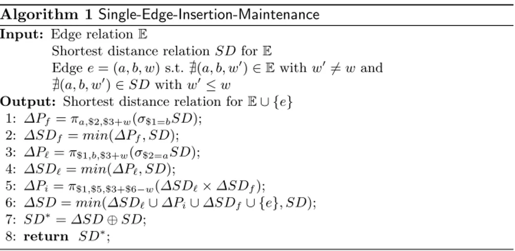
Algorithm 1 deals with the insertion of a single edge. We point out that the algorithm (as well as all the other algorithms proposed in this paper) is written in a form that eases presentation without applying optimizations to relational algebra expressions. However, relational DBMSs have full-fledged query optimization techniques to easily optimize the code—indeed, this is one of the advantages of relying on a relational DBMS.
Given the shortest distance relation SD for an edge relation E, and an edge e = (a, b, w) to be added to E, Algorithm 1 computes the shortest distance relation for E ∪ {e}. The precondition ∄(a, b, w′) ∈ E with w′6= w ensures that there does not already exist an edge from a to b.The additional precondition ∄(a, b, w′) ∈ SD with w′ ≤ w is imposed just because if it does not hold, then the insertion of e has no effect on the shortest distance relation and thus there is no need to recompute it.
The algorithm works as follows. First, it computes all the distance tu-ples obtained by concatenating e with shortest paths starting from vertex b (step 1), that is, tuples of the form (a, y, d) s.t. there is a path from a to y with distance d, the first edge along such a path is e, and the path from b to y is a shortest one (w.r.t. the original edge relation). Then, among these dis-tance tuples, the algorithm selects only those that improve on current shortest distances, that is, those tuples (a, y, d) in ∆Pf s.t. either there is no shortest path from a to y in SD or there is one with distance greater than d (step 2). Next, two analogous steps are performed: first, shortest paths ending in vertex a are concatenated with e (step 3), yielding tuples of the form (x, b, d) s.t. there is a path from x to b with distance d, the last edge along such a
20 3 Shortest Distances Maintenance on DBMS Algorithm 1 Single-Edge-Insertion-Maintenance Input: Edge relation E
Shortest distance relation SD for E
Edge e = (a, b, w) s.t. ∄(a, b, w′) ∈ E with w′6= w and ∄(a, b, w′) ∈ SD with w′≤ w
Output: Shortest distance relation for E ∪ {e} 1: ∆Pf = πa,$2,$3+w(σ$1=bSD); 2: ∆SDf = min(∆Pf, SD); 3: ∆Pℓ= π$1,b,$3+w(σ$2=aSD); 4: ∆SDℓ= min(∆Pℓ, SD); 5: ∆Pi= π$1,$5,$3+$6−w(∆SDℓ× ∆SDf); 6: ∆SD = min(∆SDℓ∪ ∆Pi∪ ∆SDf∪ {e}, SD); 7: SD∗= ∆SD ⊕ SD; 8: return SD∗;
path is e, and the path from x to a is a shortest one (w.r.t. the original edge relation); then, among the tuples in ∆Pℓ, the algorithm selects only those that improve on shortest distances in SD (step 4).
After that, the distance tuples obtained at steps 2 and 4 (which correspond to path whose first or last edge is e, respectively) are combined via a Cartesian product (step 5). Specifically, this step computes a relation ∆Piby combining each tuple (x, b, d1) in ∆SDℓwith each tuple (a, y, d2) in ∆SDf so as to get a tuple (x, y, d1+d2−w). Notice that the distance of tuples in ∆Piis diminished of w because e is taken into account both in tuples of ∆SDℓ and in tuples of ∆SDf.
Finally, the algorithm selects those tuples in ∆SDℓ∪ ∆Pi∪ ∆SDf∪ {e} that improve on the shortest distances in SD (step 6) and incorporates them into SD (step 7). The following example illustrates how Algorithm 1 works. Example 3.2. Consider the directed graph in Figure 3.3 (left) whose shortest distance relation SD is represented in Figure 3.3 (right).
d e c 1 a b 1 3 1 a c d e b 1 1 3 1 4 5 4 2
Fig. 3.3. A graph (left) and the corresponding shortest distances (right).
Suppose we add the edge (c, d, 1). Figure 3.4 shows different relations com-puted by Algorithm 1 in steps 1–5, namely ∆SDf = {(c, e, 2)} (red edge),
3.2 Incremental Maintenance of All-Pairs Shortest Distances 21 ∆SDℓ= {(b, d, 2), (a, d, 3)} (green edges), and ∆Pi= {(b, e, 3), (a, e, 4)} (pur-ple edges). d e c 1 1 a b 1 1 4 3 2 3 2 2
Fig. 3.4. Intermediate steps of Algorithm 1.
Among these new tuples, Algorithm 1 selects those that improve on current shortest distances (step 6)—intuitively, the algorithm selects the colored edges in Figure 3.4 which are not in Figure 3.3 (right) or are in Figure 3.3 (right) with a greater distance. Finally, the selected tuples are incorporated into the shortest distance relation (step 7). Figure 3.5 shows the updated graph and the new shortest distances.
a c d e b 1 1 3 1 1 a c d e b 1 1 2 1 1 3 4 3 2 2
Fig. 3.5. Updated graph (left) and the corresponding shortest distances (right).
Theorem 3.3. Given an edge relation E, the shortest distance relation SD for E, and an edge e, Algorithm 1 computes the shortest distance relation for E ∪ {e}.
Proof. Let En = E ∪ {e} and SDn be the shortest distance relation for En. We start with two observations used in the following. First, if a distance tuple (x, y, d) is in SD∗, then there is a path from x to y in E
nwhose distance is d— indeed, this property holds also for ∆Pf, ∆SDf, ∆Pℓ, ∆SDℓ, ∆Pi, and ∆SD. Second, SD∗does not contain two distance tuples (x, y, d
1) and (x, y, d2) s.t. d16= d2 (to see why, it suffices to look at steps 6–7 and the definitions of min and ⊕).
22 3 Shortest Distances Maintenance on DBMS Soundness (SD∗ ⊆ SD
n). Let (x, y, d) ∈ SD∗. As noticed above, this means that there is a path from x to y in En; thus, there must be a shortest one too, which implies that a distance tuple (x, y, d′) is in SD
n. We show that d = d′. One of the following two cases must occur.
(1) There is a shortest path r′ from x to y in E
n(its distance is d′) which does not go through e. Since r′ goes only through edges in E, then (x, y, d′) ∈ SD. Since ∆SD contains distance tuples corresponding to paths in Enthat strictly improve on shortest distances in SD (step 6), then there is no distance tuple (x, y, d′′) in ∆SD. Since SD∗ = ∆SD ⊕ SD (step 7), then (x, y, d′) ∈ SD∗. Hence, d = d′.
(2) Every shortest path from x to y in En (whose distance is d′) goes through e. Let r′ be one of such shortest paths. Then, e is either (i) the first edge of r′, or (ii) the last edge of r′, or (iii) an intermediate edge of r′. Notice that in case (i) the subpath of r′ that goes from b to y is a shortest path in E
n and also in E (because r′ does not go though e twice); in case (ii) the subpath of r′ that goes from x to a is a shortest path in E
nand also in E; in case (iii) the subpath of r′ that goes from x to a and the subpath of r′ that goes from b to y are shortest paths in En and also in E. Now it is easy to see that a distance tuple for r′ is computed at step 1 (resp. 3 and 5) when case (i) (resp. (ii) and (iii)) holds. In particular, in case (iii), since every shortest path from x to y in En goes through e, it must be the case that every shortest path from x to b in En has e as last edge, and every shortest path from a to y in En has e as first edge, and thus a distance tuple for r′ is computed at step 5. Notice that since every shortest path from x to y in En goes through e, this is the case where the insertion of e strictly improves the shortest distance from x to y. Thus, (x, y, d′) belongs to ∆SD (step 6) and SD∗ (step 7). Hence, d = d′. Completeness (SD∗ ⊇ SD
n). Consider a distance tuple (x, y, d) in SDn. If there is a shortest path r from x to y in En (its distance is d) that does not go through e, then (x, y, d) ∈ SD. This means that ∆SD does not contain a distance tuple (x, y, d′) because distance tuples in ∆SD
ℓ∪ ∆Pi∪ ∆SDf∪ {e} correspond to paths in SDnand thus do not strictly improve on p (see step 6). Hence, (x, y, d) ∈ SD∗ (see step 7). If every shortest path from x to y in En goes through e, then it can be verified that (x, y, d) ∈ SD∗ by applying the
same reasoning used in part (2) above. ✷
Single edge deletion
The algorithm to handle the deletion of a single edge consists of two phases, the first one performed by Algorithm 2 and the second one carried out by Al-gorithm 3. Roughly speaking, AlAl-gorithm 2 deletes from SD shortest distances whose corresponding paths might go through the deleted edge e. Subsequently, Algorithm 3 recomputes the new shortest distances between vertices affected by the deletion of e.
The precondition e ∈ (E∩SD) is to consider only significant cases: if e /∈ E then no edge is effectively deleted from the graph, whereas if e = (a, b, w) /∈
3.2 Incremental Maintenance of All-Pairs Shortest Distances 23 SD then there is a path from a to b not using e and with a distance strictly lower than w—in this case, the deletion of e does not affect any shortest distance (recall that we consider non-negative weights).
Algorithm 2 Single-Edge-Deletion-Maintenance Input: Edge relation E
Shortest distance relation SD for E Edge e=(a, b, w) s.t. e ∈ (E ∩ SD)
Output: Shortest distance relation for En= E − {e} 1: ∆Pf = πa,$2,$3+w(σ$1=bSD); 2: ∆SDf = (SD ∩ ∆Pf) − (En∪ (π$1,$5,$3+$6(En ✶ $2=$1SD))); 3: ∆Pℓ= π$1,b,$3+w(σ$2=aSD); 4: ∆SDℓ= (SD ∩ ∆Pℓ) − (En∪ (π$1,$5,$3+$6(SD ✶ $2=$1En))); 5: ∆Pi= π$1,$5,$3+$6−w(∆SDℓ× ∆SDf); 6: ∆SDi= SD ∩ ∆Pi; 7: SD−= ∆SD ℓ∪ ∆SDf ∪ ∆SDi∪ {e}; 8: SD = SD − SD−; 9: SD+= Recalculate(E n, SD−, SD); 10: SD∗= SD ∪ SD+; 11: return SD∗
Algorithm 2 works as follows. First, it computes all the distance tuples ob-tained by concatenating e with shortest paths starting from vertex b (step 1), that is, tuples of the form (a, y, d) s.t. there is a path from a to y with distance d, the first edge along such a path is e, and the path from b to y is a shortest one (w.r.t. the original edge relation). Among these tuples, the algorithm se-lects those that are shortest distances and for which there does not exist an alternative path having the same (minimum) cost (step 2).
Next, two analogous steps are performed: the algorithm computes all the distance tuples obtained by concatenating shortest paths ending in vertex a with e (step 3) and selects those that are shortest distances and for which there does not exist an alternative path having the same (minimum) cost (step 4).
Then, the tuples computed at step 4 (corresponding to paths where the last edge is e) are combined with the tuples computed at step 2 (corresponding to paths where the first edge is e) via a Cartesian product (step 5). Analogous to step 5 of Algorithm 1, since edge e is taken into account twice, the distance of the tuples obtained from the Cartesian product is diminished of w.
Among the tuples computed at step 5, only those that are shortest dis-tances are kept (step 6). The shortest disdis-tances computed in steps 2, 4 and 6, together with edge e, are stored in relation SD− (step 7) and deleted from SD (step 8).
24 3 Shortest Distances Maintenance on DBMS
Finally, Algorithm 3 is called (step 9); this algorithm computes the new shortest distances for paths in SD− (provided that they still exist) and the new shortest distances are added to SD (step 10).
Algorithm 3 Recalculate Input: Edge relation En
Deleted distances SD− Shortest distance relation SD Output: Relation SD+; 1: ∆P = (En∪ (π$1,$5,$3+$6(En ✶ $2=$1SD)))$1=$1∧$2=$2⋉ SD −; 2: ∆SD = min(∆P ) 3: SD+= ∆SD; 4: while ∆SD 6= ∅ do 5: ∆P = π$1,$5,$3+$6(En ✶ $2=$1∆SD)$1=$1∧$2=$2⋉ SD −; 6: ∆SD= min(∆P, SD+); 7: SD+= ∆SD ⊕ SD+; 8: end while 9: return SD+
Algorithm 3 computes the new shortest distances (when they exist) for the endpoints of the distance tuples in SD−(recall that SD− are the shortest distances that have been deleted by Algorithm 2). First, it adds to En all the distance tuples obtained by concatenating edges in En with shortest paths in the updated shortest distance relation SD (step 1). Indeed, only those distance tuples whose endpoints are in a tuple of SD− are kept and stored in ∆P . Among these distance tuples, the minimum ones are selected (step 2) and added to SD+ (step 3)—SD+ is the set of distance tuples that will be eventually returned by the algorithm (and added to the shortest distance relation by Algorithm 2).
Then, SD+ is iteratively updated as follows (steps 4–8). The algorithm computes all the distance tuples obtained by concatenating edges in En with tuples in ∆SD, and keeps only those whose endpoints are in a tuple of SD− (step 5). Among these, only distance tuples that improve on shortest distances in SD+ are kept (step 6) and incorporated into ∆SD+ (step 7). An example is provided below.
Example 3.4. Consider the graph and the corresponding shortest distances of Figure 3.5. Suppose we delete the edge (c, d, 1) from the graph.
The shortest distances affected by this deletion are marked with dashed links in Figure 3.6 (left) and are obtained at steps 1–7 of Algorithm 2 similar to the intermediate steps of Algorithm 1 depicted in Figure 3.4. Such shortest distances are deleted from the current shortest distance relation. After that, Algorithm 3 tries to recompute such shortest distances by iteratively updating ∆SD. Figure 3.6 (right) shows the new shortest distances computed by
Algo-3.2 Incremental Maintenance of All-Pairs Shortest Distances 25 d e c 1 1 a b 1 1 4 3 2 3 2 2
Andiamo
Via cosa
d e c 1 a b 1 1 5 4 4 3 2Fig. 3.6. Affected SDs (left) and new SDs (right).
rithm 3 highlighting those obtained at the initialization of ∆SD (green edges) and those computed at successive iterations (purple edges). As expected, we obtain the original shortest distances reported in Figure 3.3 (right).
Theorem 3.5. Given an edge relation E, the shortest distance relation SD for E, and an edge e, Algorithm 2 computes the shortest distance relation for E − {e}.
Proof. Let En = E − {e} and SDn be the shortest distance relation for En. Notice that each iteration of the loop in Algorithm 3 computes shortest dis-tances that strictly improve on the currently computed ones. As we consider non-negative edge weights, the number of iterations is finite. Thus, Algo-rithm 3 and consequently AlgoAlgo-rithm 2 terminate. Notice that (x, y, d) ∈ SD− iff (x, y, d) is in the input relation SD and one of the following conditions holds: (i) there is a shortest path from x to y in E whose first edge is e and there is no shortest path from x to y in En with distance d (see steps 1–2); (ii) there is a shortest path from x to y in E whose last edge is e and there is no shortest path from x to y in En with distance d (steps 3–4); (iii) there is a shortest path from x to y in E where e is an intermediate edge and for the two subpaths starting from and ending in e conditions (i) and (ii) apply, respectively (steps 5–6); (iv) e = (x, y, d) (step 7).
Soundness (SD∗ ⊆ SD
n). Let (x, y, d) ∈ SD∗. This means that there exists (x, y, d′) in the original SD. (1) If there is a shortest path from x to y in E that does not go through e, then (x, y, d′) ∈ SD
n. Conditions (i)–(ii) above do not apply. If none of conditions (iii)–(vi) applies, then (x, y, d′) is not in SD−, remains in SD, and is in SD∗. If one of conditions (iii)–(vi) holds, then (x, y, d′) ∈ SD−and it is easy to see that (x, y, d′) is computed by Algorithm 3 as it tries to compute deleted shortest distances using only edges in En. As SD∗does not contain two distinct distance tuples (x, y, d
1) and (x, y, d2), then d = d′. (2) If every shortest path from x to y in E goes through e, then one of conditions (i)–(iv) applies and thus the shortest distance from x to y in Enis correctly computed by Algorithm 3 as it computes deleted shortest distances using only edges in En.
26 3 Shortest Distances Maintenance on DBMS Completeness (SD∗ ⊇ SD
n). Let (x, y, d) ∈ SDn. This means that there exists (x, y, d′) in the original SD. (1) If d′= d, then there is a shortest path from x to y in E that does not go through e. Thus, the same reasoning used in part (1) above can be applied to show that (x, y, d)′ is not in SD−, remains in SD, and therefore is in SD∗. (2) If d′ < d, then every shortest path from x to y in E goes through e. Thus, as one of conditions (i)–(iv) applies, then (x, y, d′) ∈ SD−. Finally, (x, y, d′) is computed by Algorithm 3 and thus is in SD∗.
✷ Pang et al.’s algorithms
We briefly discuss the incremental maintenance algorithms proposed in [52] to find the shortest distance between every pair of vertices after single-edge insertion and deletion. The Algorithm 4 for edge insertion is fairly simple and works as follows. When inserting edge (a, b) with distance w > 0, the shortest distances formed by any path from node x through (a, b) to y could be affected; such paths are computed via a Cartesian product and stored in ∆P (step 1). Then, among these distance tuples, the algorithm selects only those that improve on current shortest distances, that is, those tuples (x, y, d) in ∆P s.t. either there is no shortest path from x to y in SD or there is one with distance greater than d (step 2). Finally, tuples of SD that no longer express shortest distance are updated with the new value (step 3).
Algorithm 4 Insertion - Pang et al. [52]
Input: Edge relation E; for each vertex v, the tuple (v, v, 0) is in E Shortest distance relation SD for E
Edge (a, b, w)
Output: Shortest distance relation for E ∪ {(a, b, w)} 1: ∆P = π$1,$5,$3+$6+w(σ$2=a(SD) × σ$1=b(SD)) 2: ∆SD = min(∆P, SD);
3: SD = ∆SD ⊕ SD; 4: return SD;
The Algorithm 5 for edge deletion is clearly more involved. First, it com-putes all the distance tuples obtained by concatenating (a, b) with shortest paths ending in a and those starting from node b (step 1), that is, tuples of the form (x, y, d) s.t. there is a path from x through (a, b) to y with distance d, and the paths from x to a and from b to y are the shortest ones (w.r.t. the original edge relation). Among these tuples, those that are shortest distances are stored in SD−(step 2), while the shortest distance tuples that do not use the deleted edge (a, b) are stored in the relation Trust (step 3). Edge (a, b) is then removed from the edge relation (step 4). At this point, Algorithm 5 starts computing the new shortest distances. In ∆P are stored the new tu-ples (x, y, d), whose endpoints are in a tuple of SD−, expressing that there
3.2 Incremental Maintenance of All-Pairs Shortest Distances 27 exists a path between node x and y with distance d, but d may not be the shortest (step 5). Among these distance tuples, the minimum ones are selected (step 6) and added to the tuples in Trust, forming eventually the resulting shortest distance relation (step 7).
Algorithm 5 Deletion - Pang et al. [52]
Input: Edge relation E; for each vertex v, the tuple (v, v, 0) is in E Shortest distance relation SD for E
Edge (a, b, w)
Output: Shortest distance relation for E − {(a, b, w)} 1: ∆P = π$1,$5,$3+$6+w(σ$2=a(SD) × σ$1=b(SD)); 2: SD−= ∆P ∩ SD; 3: T rust = SD − SD−; 4: E = E − {(a, b, w)}; 5: ∆P = (π$1,$8,$3+$6+$9((T rust ✶$2=$1E) ✶$5=$1T rust)) ⋉ $1=$1∧$2=$2SD −; 6: SD+= min(∆P ) 7: SD = T rust ∪ SD+; 8: return SD
3.2.2 Multiple Edges Management
In this section, we provide algorithms to update the shortest distance relation after the insertion or deletion of multiple edges. Obviously, the insertion of k edges might be handled by calling k times Algorithm 1, and the deletion of multiple edges might be analogously handled. However, the algorithms we propose in this section leverage the information about the entire set of edges to be inserted or deleted to maintain the shortest distance relation in a more efficient way.
The core idea is to identify paths affected by the insertions/deletions start-ing from the vertices that are one hop far from the inserted/deleted edges and propagating changes farther only if necessary. If the insertion/deletion of an edge e = (a, b, w) does not influence the shortest distance from a to b, then no updates need to be propagated. On the other hand, if the shortest distance from a to b changes, this may in turn affect the shortest distances of a’s and b’s neighbors (because their shortest paths may use edge e). In this case, our algorithms update the shortest distance from a to b and propagate the vari-ations farther only if a’s and b’s neighbors are really affected. For instance, if there is no path from a to b after the deletion of e, but their neighbors still have the same shortest distances (because of alternative paths), then the algorithms do not look at farther vertices. On the other hand, if changes are propagated, vertices that are two hops from e are considered by applying the same reasoning.
28 3 Shortest Distances Maintenance on DBMS
Moreover, proceeding one hop at a time allows the algorithms to combine the effects of the different edges to be inserted/deleted, reducing the compu-tational effort w.r.t. individually handling them one at a time.
In order to deal with the insertion and deletion of multiple edges, we need to extend the algorithms proposed in Section 3.2.1.
One extension regards the schema of the auxiliary relations used in the algorithms. We will use relations ∆Pf, SDf, ∆SDf, ∆Pℓ, SDℓ, and ∆SDℓ, whose schema has been enriched for algorithmic purposes. Specifically, ∆Pf, SDf, and ∆SDf contain extended distance tuples of the form (x, y, d, a, w) meaning that there is an edge from x to a with weight w, a path r from a to y, and d = w + ω(r). In other words, (x, y, d, a, w) means that there exists a path from x to y, having distance d, and whose first edge is (x, a, w).
On the other hand, ∆Pℓ, SDℓ, and ∆SDℓcontain extended distance tuples of the form (x, y, d, a, w) meaning that there is a path r from x to a, an edge from a to y with weight w, and d = ω(r) + w. In other words, (x, y, d, a, w) means that there is a path from x to y, having distance d, and whose last edge is (a, y, w).
Multiple edges insertion
Algorithm 6 is an extension of Algorithm 1 that is able to handle the insertion of multiple edges at once. It takes as input an edge relation E, the shortest distance relation SD for E, and a set of edges ∆E to be added to E. The output is the shortest distance relation for E ∪ ∆E.
The algorithm first computes a subset ∆Esof ∆E containing those edges (a, b, w) s.t. w is less than the shortest distance from a to b in the input relation SD (step 1); ∆Es is then incorporated into SD (step 2). After this pre-processing phase, the updating phase starts.
More in detail, the algorithm initially considers paths composed by two edges, where the first one belongs to ∆Es (step 3). For each of these paths having a distance lower than the current shortest distance (steps 6–8), the algorithm considers longer paths (in terms of number of edges) obtained by adding one more edge to the right (step 9). The process is repeated until no further lower distances are obtained (steps 5–10).
Then, the algorithm proceeds in a similar way but adding edges to the left. More specifically, it first considers paths with two edges where the last one belongs to ∆Es (step 11) and then iteratively adds further edges to the left as long as paths improving on current shortest distances can be derived (steps 13–18).
After the iterative steps described above, SDf (resp. SDℓ) contains ex-tended distance tuples referring to paths whose first (resp. last) edge belongs to ∆Es. In addition, each extended distance tuple belonging to these sets maintains information about the first or last edge being used and its weight. This information is used in the next step (step 19), where an extended dis-tance tuple of SDℓis combined with an extended distance tuple of SDf iff the